Neural Decoder for Topological Codes using Pseudo-Inverse of Parity Check MatrixPreprint: AIP/123-QED
Abstract
Recent developments in the field of deep learning have motivated many researchers to apply these methods to problems in quantum information. Torlai and Melko first proposed a decoder for surface codes based on neural networks. Since then, many other researchers have applied neural networks to study a variety of problems in the context of decoding. An important development in this regard was due to Varsamopoulos et al. who proposed a two-step decoder using neural networks. Subsequent work of Maskara et al. used the same concept for decoding for various noise models. We propose a similar two-step neural decoder using inverse parity-check matrix for topological color codes. We show that it outperforms the state-of-the-art performance of non-neural decoders for independent Pauli errors noise model on a 2D hexagonal color code. Our final decoder is independent of the noise model and achieves a threshold of . Our result is comparable to the recent work on neural decoder for quantum error correction by Maskara et al.. It appears that our decoder has significant advantages with respect to training cost and complexity of the network for higher lengths when compared to that of Maskara et al.. Our proposed method can also be extended to arbitrary dimension and other stabilizer codes.
Keywords:
Quantum Error Correction, Neural Networks, Deep Learning, Topological Codes, Surface Codes, Stabilizer Codes, Color Codes.pacs
03.67.PpI Introduction
In quantum computers basic unit of information is a qubit. Qubits are highly susceptible to noise. Hence to protect the information, we use quantum codes. A very popular class of quantum codes for protecting information are topological quantum codes. In this paper we focus on a subclass of topological codes in two spatial dimensions called color codes Bombin and Martin-Delgado 2006a. To correct the impact of noise on the encoded information we would need a decoder. Novel decoding algorithms for 2D color codes have been proposed earlier in Wang et al. 2009; Sarvepalli and Raussendorf 2012; Delfosse 2014; Bombin et al. 2012. However, these are not optimal and do not meet the theoretical bounds for performance. Furthermore, designing decoders for non-Pauli noise is a challenging problem.
Recent developments in the fields of machine learning (ML) and deep learning (DL) have motivated many researchers to apply these methods to decoding quantum codes. Torlai and Melko were the first to propose a decoder for surface codes based on neural networks Torlai and Melko 2017. Since then, many other researchers have applied neural networks to study a variety of problems in the context of decoding Torlai and Melko 2017; Varsamopoulos et al. 2018a; Krastanov and Jiang 2017; Baireuther et al. 2019; Chamberland and Ronagh 2018; Davaasuren et al. 2018; Jia et al. 2019; Breuckmann and Ni 2018; Baireuther et al. 2018; Maskara et al. 2018.
In this paper we only focus on decoding of color codes using neural networks. Early work based on neural networks attempted to the solve the problem using using neural networks entirely. These did not beat the non-neural methods. An important development in this context was due to Varsamopoulos et al. 2018a who proposed a combination of neural networks and non-neural decoders. More precisely, they have a two-step decoder where in the first-step, they estimate an pure-error and in the second-step, they use a neural network which estimates the logical. In their recent work Varsamopoulos et al. 2018b, they mention that any simple decoder can be used in the first-step. The authors of Davaasuren et al. 2018 claim that the work of Varsamopoulos et al. 2018a is a special case of their generalized framework of building neural networks for decoding stabilizer codes. The works of Baireuther et al. 2019; Chamberland and Ronagh 2018 attempt to use neural networks for fault-tolerant setting. The most relevant work to ours is Maskara et al. 2018 in which a similar combination of two decoders is employed to conclusively demonstrate the usefulness of neural decoders. They proposed a neural decoder with progressive training procedure that outperformed previously known decoders for 2D color codes.
In this work, we propose a similar two-step neural decoder for color codes and study its performance for the hexagonal color code on the torus. We propose two variations, one which achieves a threshold of and another with an important modification that achieves a near optimal threshold for independent bit-flip/phase-flip noise model. This modification can be incorporated in other neural network based decoders and could be of potentially larger importance. The main challenge involved with neural networks is determining the correct architecture in order to improve the overall threshold. We model our non-neural decoder in a simple way and show the advantages of doing so with the improvement in performance of the neural decoder, the reduction in cost of training and scaling associated with the distance of the code. Our main contributions are,
- 1)
We propose a two-step neural decoder with a simple decoding procedure in the first-step, applicable for all stabilizer codes.
- 2)
We suggest an alternative approach on combining the non-neural and the neural decoder which can be incorporated in other neural network based decoders.
- 3)
Our proposed approaches seem to have significant advantages with respect to training cost and complexity of the network for higher lengths when compared to the previous work of Maskara et al. Maskara et al. 2018.
The paper is organized as follows. We review the necessary background on Quantum Error Correction (QEC), ML and DL in Section II. We then describe our approach, the neural architecture used in detail and compare it with related work in Section III. In Section IV, we point out valuable insights from our work and conclude in Section V.
II Background
In this section, we summarize the necessary background on Quantum Error Correcting Codes (QECC). In Section II.1, we briefly review stabilizer codes. In this paper we focus on color codes which are introduced in Section II.2. Lastly, in the Section II.3 we describe basics of ML and DL with emphasis on deep learning by discussing the various components in a neural network which can be changed depending on the problem to be solved.
II.1 Stabilizer codes
In this section, we briefly review stabilizer codes. Recall, that the Pauli group on a single qubit is generated by the Pauli matrices . The group consists of tensor products on single qubit Pauli operators, . A stabilizer code is defined by an abelian subgroup , such that . The codespace , is joint +1-eigenspace of .
An stabilizer code encodes logical qubits into physical qubits and its stabilizer will have independent generators. We assume that is generated by , where and are linearly independent.
Let be the centralizer of i.e. the set of all Pauli operators that commute with all the elements of . Let , where and denote the logical and operators of the code. Also, commute if and anti-commute if . Let .
We define another set of operators called the pure errors, such that and commute if and anti-commute if . The pure errors commute with each other and also with the logical operators. Let . Note that together form a generating set for .
An error operator, will anti-commute with at least one stabilizer operator in group . If anti-commutes with the stabilizer , the syndrome bit is one and zero otherwise. By calculating the syndrome values for all the stabilizer generators, the syndrome vector can be written as, where .
We can write the error operator up to a phase as proposed in Duclos-Cianci and Poulin 2010. Here , and . Note that the operators , , depend on the error . The effect of is trivial, implying two error patterns and will have same effect on codespace. introduces an equivalence relation in error operators and hence finding is of little interest. Also, given syndrome , we can uniquely identify but identifying is a difficult task. The problem of error correction for stabilizer codes is finding the most likely given the syndrome vector . Mathematically, we can write this as,
| (1) |
Decoding can be thought of as a classification problem. We have classes, which is exponential in and this reformulation of the decoding problem as a classification is not much help for large . Fortunately, surface codes and color codes have fixed number of logical operators for any length and this reformulation can be taken advantage of. However, this is not sufficient, note that the computation of the probabilities in Eq. (1), requires the summation over terms which is of exponential complexity. So the reformulation of the decoding as a classification is not adequate, but further work is required to fully exploit this perspective.
II.2 Color codes
Topological codes are a class of stabilizer codes where the stabilizer generators are spatially local. Popular examples of topological codes are Toric codes Kitaev 2003 and Color codes Bombin and Martin-Delgado 2006a. Color codes are defined using a lattice embedded on a surface. Every vertex is trivalent and faces are 3-colorable.
Qubits are placed on the vertices of the lattice and for each face , we define an and type operators called the face operators. We define the the stabilizers as,
All and type operators corresponding to every face generate the stabilizers of the color code. The color code on a hexagonal lattice with periodic boundary is shown in the Fig. 1. It encodes four logical qubits Bombin and Martin-Delgado 2006a.
II.3 Machine Learning and Deep Learning
II.3.1 An overview of Machine Learning
In traditional computing, algorithms are sets of explicitly programmed instructions which perform a specific task as to give out correct output for the given input. ML is a concept to learn patterns from data through statistical analysis and make predictions without those rules being programmed explicitly. These ML algorithms are therefore data driven methods and the process of learning these rules or patterns is called training of the ML model. Training is essentially an optimization process minimizing an objective function called the loss function. This loss function plays an important role in the algorithm learning these patterns and making good predictions.
There are many such algorithms for solving problems of classification, regression etc and some of them are mentioned in Kotsiantis 2007; Domingos 2012. Any function can be used as a loss function but they need not necessarily help the algorithm learn. There exist specific loss functions which are mathematically proven to be apt for solving each of the above mentioned tasks. Mathematically, the core of any ML algorithm is to estimate the parameters of a function or set of functions which solve the given task.
Training can be classified into two types, supervised learning and the unsupervised learning. The requirement for supervised learning is labeled dataset of inputs and the corresponding true outputs . These true outputs are sometimes referred to as ground truth. The ML algorithm will learn the patterns in the data by this information of input and correct output during training and tries to predict , the correct prediction during testing. Eg. Classification, Regression. In unsupervised learning, we still have input data but the corresponding ground truth information is not present. The ML algorithm is required to learn the patterns from the input data alone without the information of the ground truth. Eg. Clustering.
II.3.2 An overview of Deep Learning
Neuron and Activation functions:
A neuron is an element which takes an input and performs the operation as shown in the Fig. 2.
The parameters are called weights and the parameter is called the bias.
Each element of these vectors and are real numbers. The function is a non-linear function and is called the activation function. Some common activation functions include Sigmoid, TanH, ReLU (Rectified Linear Unit) etc as shown in the Fig. 3 and are exhaustively discussed in Goodfellow et al. 2016.
Deep Learning (DL) is a method in ML to estimate the parameters of a function using a combinations of this basic element neuron. It is common to address the combined set of parameters in and as weights or parameters and we follow this same convention in our subsequent discussion. The activation function plays a very crucial role in DL since without that, a neuron just performs a linear operation.
Architectures: Different combinations of these basic neurons result in different architectures. Some of such famous architectures are Fully-Connected Networks (FC), Convolutional Neural Networks (CNN), Recurrent Neural Networks (RNN) etc. All these architectures comprise of layers which are again a combination of neurons. Essentially, these architectures can be characterized by these layers.
Fully-connected Network: We briefly describe the FC architecture which we use in our work as shown in Fig. 4. Any FC network has an input layer, an output layer and hidden layers. Each layer comprises of neurons and each neuron is connected to every other neuron in the adjacent layers. Connectedness implies that each neuron receives the output of the neurons it is connected to in the previous layer and it passes the output of itself to all the connected neurons in the next layer. All the neurons in every layer follow this rule except that the neurons in the input layer take the input from the data and the neurons in the output layer give us the final prediction. The input data and the output prediction varies from problem to problem. In a simple image classification task, the input data is the image and the output is the class label. As mentioned before, the non-linear function plays a crucial role in the success of DL in estimating complicated functions efficiently, making DL a very powerful tool.
Loss functions: The loss function plays a prominent role in the performance of any DL model. It is calculated between the true label or the ground truth and the prediction made by the network . The training procedure as described next ensures that the predictions made by the network get closer to the ground truth by minimizing the loss function as the training progresses. For regression problem, commonly used loss functions are are and norms as defined below.
For classification problems, cross-entropy () is used as the loss function which is defined in the following equation.
We use this cross-entropy loss in our work since QEC can be viewed as a classification problem as described in Section III.1. We discuss the reasons for using this loss in Section III.3.
Training: Training is nothing but estimating the values of the weights of the network which minimizes the chosen loss function for the given training data or the input-output pairs. One of the traditional method of updating the weights to minimize a function is Gradient Descent (GD) algorithm. It is an iterative algorithm which tries to optimize the objective function and in our case minimize the loss function through updating the weights of the network in each iteration by following the update rule defined below, as discussed in Goodfellow et al. 2016.
Here, are the weights of the network at the iteration. The weights are initialized randomly. There are many methods to initialize these weights and we mention about them shortly. The parameter is called the learning-rate and is a hyper-parameter. There are many such hyper-parameters and we also discuss them later in this section. The speed with which and the optima to which the model converges to, depends on .
The gradient descent algorithm requires us to train on the entire training dataset at once, i.e calculate the average loss for all the inputs in the dataset and update the weights. Since that is not usually computationally feasible, a popular variant of it called the Stochastic Gradient Descent (SGD) is employed. Instead of training on the entire dataset at once, the model is trained on small batches of data until all the training data is exhausted which completes one epoch. The size of this batch is called the batch-size as mentioned in Goodfellow et al. 2016. For example, if the entire dataset contains data points, then GD requires us to calculate the average loss on all the inputs and then update the weights in one iteration. In SGD, say we choose the batch-size to be , then data points are chosen randomly from the entire dataset of . The average loss is calculated for that batch of and the weights are updated. This completes one iteration. In the second iteration, another set of data points are chosen randomly from the remaining data points and the rest of the procedure follows. In this example, a total of iterations are required to exhaust the entire dataset which completes an epoch.
One of the major limitation of gradient descent and its variants is that it does not guarantee convergence to global optima. Since the loss is calculated between the true label and the prediction of the network , it is indirectly a function of the weights of the network , since is a function of and .
Weight initialization and back-propagation: Before training, the weights of the NN, are randomly initialized. Weight initialization plays a crucial role in training and performance of the NN. There are many weight initialization methods but the popular ones are proposed by He et al. 2015 and Glorot and Bengio 2010. These methods have been shown to perform well in solving classification problems. Training neural networks can be incredibly costly with GD or SGD but with the use of a dynamic programming based algorithm called the back-propagation algorithm, the cost of training reduces significantly as discussed in Goodfellow et al. 2016. The back-propagation algorithm also uses gradient-descent but stores the values of the gradients to the current layer in order to calculate the gradients to the weights of the previous layer.
Optimizers: There are many variants of the SGD algorithm described above like RMSProp, AdaGrad as mentioned in Goodfellow et al. 2016 which have a modified update rule. All these rules are commonly called optimizers since they optimize the weights of our network in order to minimize the loss function. We use Adam optimizer, proposed by Kingma and Ba 2014 because of the significant improvements it offers during training and also in the performance of deep neural networks.
Hyper-parameters: As we can see, numerous design decisions are required to build a neural network like the architecture, the loss function, activation function, weight initialization, optimizer etc. Once those are selected, we have few more parameters to experiment with, listed as follows,
- i)
The number of hidden layers
- ii)
The learning rate
- iii)
The number of neurons in each layer
- iv)
The batch-size
These parameters are called hyper-parameters of the network. Choosing the right set of hyper-parameters for a give problem is one of the biggest challenges of DL. These parameters play a crucial role in both training and performance of the networks because the training procedure does not guarantee convergence to global minima of the loss function, as mentioned previously.
II.3.3 Process flow of a common DL architecture
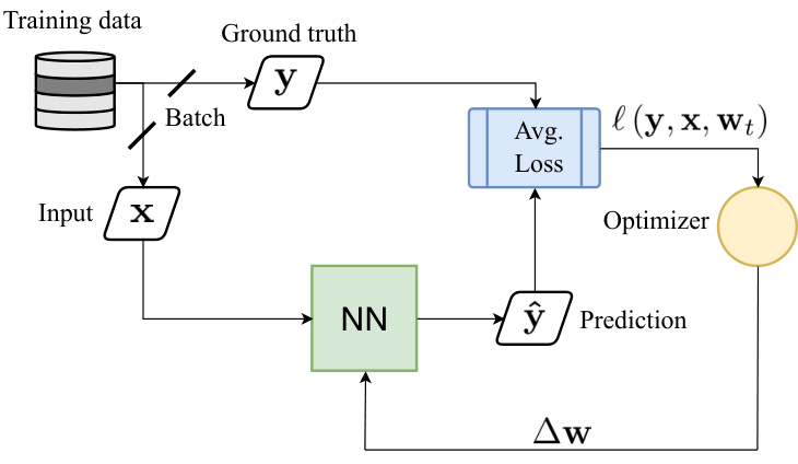
The process flow of any DL architecture can be modeled as shown in Fig. 5. The NN can be any neural network as described previously. The NN takes an input from the training data and makes a prediction . The loss is calculated between the ground truth and the prediction . The optimizer then updates the weights of the NN according to the update rule. This whole process completes one iteration during training. We repeat this process until the loss value between and saturates over multiple iterations.
II.3.4 Classification problem
In machine learning and statistics, classification is the problem of identifying to which of a set of categories or classes a new observation belongs to. This relation is statistically obtained from training data. A classification algorithm will predict the confidence score or the probability of the new observation belonging to a particular class. This can be illustrated in a dummy example of classification between domestic cats and dogs with the knowledge of their weight and length as shown in Fig. 6. The weight and height are called the features since the algorithm classifies with that information. Estimating the parameters of the line is solving the classification problem. In general the boundary could be a complicated curve and there could be multiple classes with multiple features. Commonly, these features might not be available and we have to devise algorithms to extract them from the input.
Mathematically, if we assume the feature vector to be for an observation and the total classes are the set , then the prediction is the most likely class that belongs to as defined in the following equation.
Generally, traditional ML algorithms requires us to extract these features from the input using some rules where as neural networks are known to extract them by themselves from the input directly, for example as shown in Krizhevsky et al. 2012. This helps immensely in the success of DL since the network learns to extract the important features for solving the problem, instead of us using hand coded rules to extract what we think are important features.
III Decoding Color Codes using Neural Networks
In this section, we describe our problem formulation for correction of phase errors and how the decoding can be modeled as a classification problem. For any stabilizer code, every error can be uniquely decomposed to the pure error , logical error and a stabilizer as mentioned in the Section II.1.
Given the syndrome , we can uniquely identify . Since the stabilizers form the equivalence class, the decoding problem comes down to correctly estimating given . In this work, we study CSS codes which have two types of stabilizers, and . They can be written in the matrix form as,
Phase errors create non-zero syndromes and hence we consider only stabilizers from now on. The matrix represents the stabilizers and represents the stabilizers. For 2D color codes, and in the subsequent equations, we use instead of for simplicity. Denote the binary representation of as . Then we can calculate the corresponding syndrome as,
| (3) |
The matrix is not full rank. In color code, stabilizers corresponding to faces have two dependencies as mentioned in Bombin and Martin-Delgado 2006b. We remove those two dependent stabilizers from the matrix, one stabilizer each corresponding to two different colors and denote it as which is full rank. We calculate the right pseudo-inverse of and denote it as .
| (4) |
The resultant syndrome which does not list the syndromes calculated by the removed dependent stabilizers is denoted by as shown below.
| (5) |
III.1 QEC as a classification problem
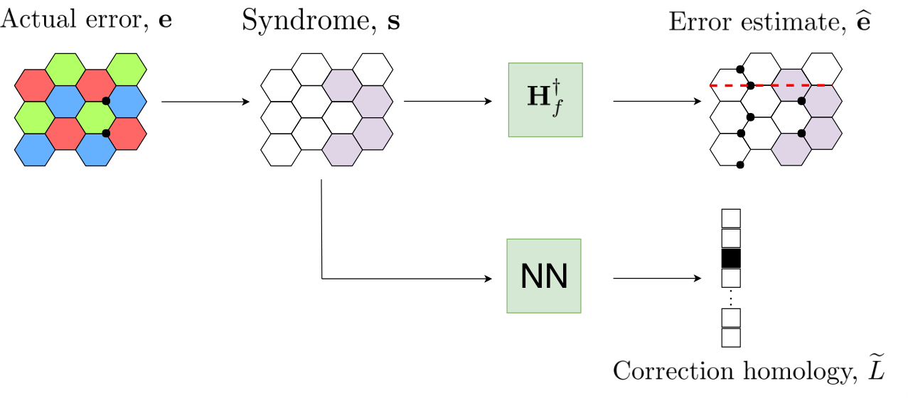
Researchers have previously studied the perspective of quantum error correction as a classification problem using neural networks Varsamopoulos et al. 2018a; Maskara et al. 2018; Chamberland and Ronagh 2018. As mentioned before, we model our decoder as a two-step process. The first-step is a simple inversion where we calculate an estimate of the actual error which has occurred. We first calculate the syndrome from Eq. (5) and then estimate , the binary representation of the operator as follows,
| (6) |
Note that the syndrome of the estimate will be same as the syndrome of . Hence, they have the same pure error .
| (7) |
This estimate computed using Eq. (6) need not be same as . This is because there exist multiple errors with the same syndrome. We have chosen one solution by fixing which is calculated only once. This makes the first-step of the decoder simple. From Eq. (7), we can conclude that the pure error is same in both and and we denote it by . Applying this initial estimate onto the system might result in logical error. This can be concluded through the following equations.
| (8) |
Here and . The reason for occurrence of in Eq. (8) is because the Pauli operators , might commute or anti-commute. This is of little interest to us because we estimate the error up to a global phase.
The homology of is same as the homology of since has a trivial homology. If we can predict the resultant homology , we can get back to the trivial state and the decoding succeeds. Since the number of homologies are fixed, this is modeled in the second-step of our decoder as a classification problem using NN. The goal of the NN is to predict given the syndrome . Our final error correction will be,
| (9) |
If the NN properly predicts this correction will restore the state up to a global phase which is evident through the following equations.
The work by Maskara et al. 2018 used a naive decoder which removes syndromes by pushing errors to the boundary in the first-step. Their neural network tries to improve upon this estimate by predicting the correction homology. Mathematically, this means that their decoder could implement different inverse for a different syndrome. In our approach, we fix the inverse in the first-step, making our initial decoder much simpler. We discuss more on this in the Section IV. The first-step decoder in Varsamopoulos et al. 2018a is to estimate the pure-error which needs to satisfy many properties. We want to emphasize that our inverse matrix in step-one gives us an error estimate which need not always be pure error. It entirely depends on the construction of . We used SageMath 11 1 http://sagemath.org, an open-source mathematics software for calculating from Eq. (4).
III.2 Neural decoder
In this section, we describe our neural decoder in the second-step. As mentioned before, we have modeled our NN in two ways and in both of them we have used a fully-connected architecture where every neuron in one layer is connected to every other neuron in the adjacent layers. The output of the network is the homology vector where each element of it represents a homology class. Since this is a classification problem, we use cross-entropy as our loss function which needs to be minimized during training. We have used Adam optimizer proposed by Kingma and Ba 2014 since it has been observed to perform better than the other optimizers in terms of convergence of the loss. We have also used 1D batch normalization layer after every layer in the network. It is proven to significantly boost the training speed as shown in Ioffe and Szegedy 2015. The activation function used for every neuron is ReLU since it has shown to perform well when compared to other functions like Sigmoid or TanH by reducing the problem of vanishing gradients as the network goes deeper as shown in Karlik and Olgac 2011; Glorot et al. 2011.
| 33 3 Number of hidden layers | 44 4 Hidden dimension factor | 55 5 Batch size | 66 6 Learning rate | 77 7 Number of training samples per each | 88 8 Total number of training samples for all combined | |
III.3 Training procedure
For the network to decode correctly, it needs to be trained. We employ a supervised training procedure where we have labeled data of input (we generate according to the noise and calculate syndromes from Eq. (3)) and the corresponding output (homology ). This output is the ground truth. Training is nothing but an optimization process where the weights of the network are optimized to minimize an objective function. This objective function is called loss function. The loss function plays a crucial role during training since certain loss functions are apt for certain problems. Since our NN needs to solve a classification problem, we use cross-entropy as our loss function. This is because given a syndrome , the NN predicts a probability distribution over all the possible classes. If we assume input is , the output of the NN is a distribution and the true distribution is , cross-entropy can be written as follows.
| (10) |
This is same as minimizing the Kullback-Liebler divergence between the distributions and up to a constant since can be written as,
and the term is a constant because it is completely determined by the true distribution . This implies that minimizing in Eq. (10) gets the distribution learned by our NN i.e, closer to the true distribution .
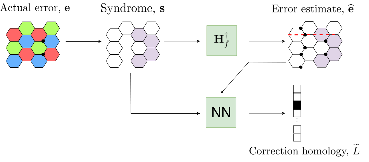
Given a syndrome vector , a trained NN should be able to correctly predict the correct correction homology class for all error rates under the threshold. In order to train a NN which is independent of the error rate, we employ a progressive training procedure as described in Maskara et al. 2018. We generate training samples at a fixed error rate in each case and we train our NN for that noise until the loss function in Eq. (10) saturates. We then move on to a higher and repeat the process for various error rates under the threshold. For our experiments (bit-flip noise), we have trained our NN for the error rates . We use Xavier normal initialization for the parameters in fully-connected layers and Gaussian normal initialization for the parameters in batch-normalization layer before we start training. We do not reinitialize the weights during the progressive training while we train on the higher . We discuss the importance of this progressive training with evidence in the Section IV. In our first approach, we use the syndrome alone as the input to the network whereas in our second approach, we use the concatenated vector of both initial estimate and the syndrome . In both cases, the network is trained to predict correction homology . Our -inverse decoder in step-one can be summarized in Alg. 1. The neural decoders can be summarized in Algs. 2, 3 for our first and second approaches respectively. The architectures for our decoders are illustrated in Figs. 7, 11 for first and second approaches respectively.
III.4 Results
We describe our simulation results for bit-flip noise model in this section. As described earlier in the Section III, our decoder is a two-step decoder where we use a naive and deterministic -inverse decoder in step-one and then improve its performance in step-two using a NN. The performance of our -inverse decoder in the step-one by itself is shown in the Fig. 9. It shows that -inverse alone is a very bad decoder since the logical error increases as the length of the code increases for a fixed . It is quite evident that this decoder does not have a threshold since the curves do not meet anywhere below the theoretical threshold of Katzgraber et al. 2009.
The performance of our neural decoder in first approach (Fig. 7) trained according to the training procedure mentioned in Section III.3 is shown in the Fig. 10(a). The fully trained NN model is independent of the and the it outperforms the previous state-of-the art methods which are not based on neural networks by Sarvepalli and Raussendorf 2012; Delfosse 2014; Bombin et al. 2012. We report that our neural decoder achieves a threshold of and is comparable to the result mentioned in Maskara et al. 2018.
In our second approach, we have given additional information of along with the syndrome vector (by concatenating them both) to our NN (Fig. 11) and saw a dramatic improvement in the threshold for small lengths, as well as a reduction in logical errors for each error rate as shown in the Fig. 10(b). The training is exactly similar to the previous case. This shows that the NN is able to understand and learn the behaviour of the -inverse decoder much better with the additional knowledge of the initial estimate and hence is able to perform better correction. This implies that the data driven methods and in particular neural networks’ performance can be improved by providing all the information available to us relevant to the problem to be solved. This modification can be incorporated into other works of building two-step decoders using neural networks and improve the overall performance.
The hyper-parameters (as described in the Section II.3) of our networks are listed in the Tables 1, 2 for first and second approaches respectively. The variation of some of them with the distance are shown in the Fig. 8 for both the approaches. The distance of the code is denoted by and the number of hidden layers in our network is denoted by . The batch size used for each length is denoted by . The number of nodes in each hidden layer are characterized by the hidden dimension factor which is equal to multiplied by the dimension of the input syndrome vector . The parameter is the number of samples required for training for each and determines the total number of samples the final trained NN has seen entirely. The parameter is the learning rate used for optimization. We used PyTorch 99 9 https://pytorch.org/, an open-source deep learning framework for training our neural networks.
| 1111 11 Number of hidden layers | 1212 12 Hidden dimension factor | 1313 13 Batch size | 1414 14 Learning rate | 1515 15 Number of training samples per each | 1616 16 Total number of training samples for all combined | |
IV Remarks and Insights
We clearly demonstrate the power of data-driven methods and in particular neural networks, through which we were able to improve the performance of a very bad decoder which does not even have a threshold. When compared to the previous state-of-the-art on neural decoders for color codes, our decoder requires significantly less training data for higher lengths like . In addition to the gains in training cost, our decoder has less complexity with respect to the number of layers and number of nodes in each layer when compared to the previous work and still achieved a comparable threshold. In Section III.3, we mentioned the importance of the progressive training. We ran our simulations by training a new NN with Xavier normal and Gaussian normal initializations for every , without employing the progressive training. The performance of that decoder with similar hyper-parameters as mentioned in the Table 1 is shown in the Fig. 12. This shows that without the progressive training, the threshold of the decoder drops to about . This is because as the increases, it would be very likely that our optimizer converges to a bad local minima. This progressive training is similar to the common practice of curriculum-learning in neural networks so that the optimizer converges to a better local minima in the hyperspace of the network weights as proposed in Bengio et al. 2009. We also report that this progressive training should be carried on till the equals the theoretical threshold and we have observed constant decrement in logical errors at all error rates. Training the model with a above the threshold is not desirable as we have seen increments in the logical errors. This concept of -inverse as a base decoder improved with a neural decoder can be effectively extended to other noise models and also to codes in higher dimension including other stabilizer codes.
Any decoder which does error correction essentially solves the equation . Since there are many solutions, it implies there exist many pseudo-inverses to . To implement a good decoder, choosing the correct inverse for a given syndrome is an important task. Different inverses must be chosen for different syndrome patterns in order to have a threshold. The choice of decoder in the step-one can be anything as long as it clears the syndrome and good decoders which have a threshold can also be chosen. In such cases, these good decoders take care of selecting the inverse depending on the syndrome. This makes these step-one decoders not entirely simple and there is a lot more for the NN to learn to improve the initial estimate. This is because the inverse selected will be different for different syndromes. In our approach, we fix the inverse though it does not have a threshold and make the step-one decoder very simple. Our NN only has to understand on inverse which is to improve the initial estimate. Intuitively, this means that the learning should be easier for our NN which can be verified empirically through the superior performance with comparatively lesser training cost and complexity when compared to Maskara et al. 2018. Our approach is applicable for any decoding problem where the equation, needs to be solved.
V Conclusion
We have demonstrated that data-driven methods like NN can perform superior decoding when compared to the traditional approaches. We propose a neural decoder with simplified non-neural part achieving a threshold of for 2D color codes. We suggest an alternative approach to combine non-neural and neural decoders reducing the logical error which can be incorporated into other NN based decoders. The drawbacks of NN based decoders are figuring out the right set of hyper-parameters for each length and practical issues of convergence of the loss when the number of trainable parameters increase. Our approach can be extended to other realistic noise models and codes in higher dimensions or other stabilizer codes.
VI Acknowledgements
The authors would like to thank Arun B. Aloshious for valuable discussions. During the preparation of this manuscript, five related preprints were made available Ni 2018; Sweke et al. 2018; Liu and Poulin 2018; Andreasson et al. 2018; Nautrup et al. 2018, however their scope and emphasis are different from our work. This work was completed when CC was associated with Indian Institute of Technology Madras as a part of his Dual Degree thesis.
References
- Bombin and Martin-Delgado (2006a) H. Bombin and M. A. Martin-Delgado, “Topological quantum distillation,” Phys. Rev. Lett. 97, 180501 (2006a).
- Wang et al. (2009) David S Wang, Austin G Fowler, Charles D Hill, and Lloyd Christopher L Hollenberg, “Graphical algorithms and threshold error rates for the 2d colour code,” arXiv preprint arXiv:0907.1708 (2009).
- Sarvepalli and Raussendorf (2012) Pradeep Sarvepalli and Robert Raussendorf, “Efficient decoding of topological color codes,” Phys. Rev. A 85, 022317 (2012).
- Delfosse (2014) Nicolas Delfosse, “Decoding color codes by projection onto surface codes,” Phys. Rev. A 89, 012317 (2014).
- Bombin et al. (2012) Hector Bombin, Guillaume Duclos-Cianci, and David Poulin, “Universal topological phase of two-dimensional stabilizer codes,” New Journal of Physics 14, 073048 (2012).
- Torlai and Melko (2017) Giacomo Torlai and Roger G. Melko, “Neural decoder for topological codes,” Phys. Rev. Lett. 119, 030501 (2017).
- Varsamopoulos et al. (2018a) Savvas Varsamopoulos, Ben Criger, and Koen Bertels, “Decoding small surface codes with feedforward neural networks,” Quantum Science and Technology 3, 015004 (2018a).
- Krastanov and Jiang (2017) Stefan Krastanov and Liang Jiang, “Deep Neural Network Probabilistic Decoder for Stabilizer Codes,” Scientific reports 7, 11003 (2017).
- Baireuther et al. (2019) P Baireuther, M D Caio, B Criger, C W J Beenakker, and T E O’Brien, “Neural network decoder for topological color codes with circuit level noise,” New Journal of Physics 21, 013003 (2019).
- Chamberland and Ronagh (2018) Christopher Chamberland and Pooya Ronagh, “Deep neural decoders for near term fault-tolerant experiments,” Quantum Science and Technology 3, 044002 (2018).
- Davaasuren et al. (2018) Amarsanaa Davaasuren, Yasunari Suzuki, Keisuke Fujii, and Masato Koashi, “General framework for constructing fast and near-optimal machine-learning-based decoder of the topological stabilizer codes,” arXiv preprint arXiv:1801.04377 (2018).
- Jia et al. (2019) Zhih-Ahn Jia, Yuan-Hang Zhang, Yu-Chun Wu, Liang Kong, Guang-Can Guo, and Guo-Ping Guo, “Efficient machine-learning representations of a surface code with boundaries, defects, domain walls, and twists,” Phys. Rev. A 99, 012307 (2019).
- Breuckmann and Ni (2018) Nikolas P. Breuckmann and Xiaotong Ni, “Scalable Neural Network Decoders for Higher Dimensional Quantum Codes,” Quantum 2, 68 (2018).
- Baireuther et al. (2018) Paul Baireuther, Thomas E. O’Brien, Brian Tarasinski, and Carlo W. J. Beenakker, “Machine-learning-assisted correction of correlated qubit errors in a topological code,” Quantum 2, 48 (2018).
- Maskara et al. (2018) Nishad Maskara, Aleksander Kubica, and Tomas Jochym-O’Connor, “Advantages of versatile neural-network decoding for topological codes,” arXiv preprint arXiv:1802.08680 (2018).
- Varsamopoulos et al. (2018b) Savvas Varsamopoulos, Koen Bertels, and Carmen G Almudever, “Designing neural network based decoders for surface codes,” arXiv preprint arXiv:1811.12456 (2018b).
- Duclos-Cianci and Poulin (2010) G. Duclos-Cianci and D. Poulin, “A renormalization group decoding algorithm for topological quantum codes,” in 2010 IEEE Information Theory Workshop (2010) pp. 1–5.
- Kitaev (2003) A.Yu. Kitaev, “Fault-tolerant quantum computation by anyons,” Annals of Physics 303, 2 – 30 (2003).
- Kotsiantis (2007) S. B. Kotsiantis, “Supervised machine learning: A review of classification techniques,” in Proceedings of the 2007 Conference on Emerging Artificial Intelligence Applications in Computer Engineering: Real Word AI Systems with Applications in eHealth, HCI, Information Retrieval and Pervasive Technologies (IOS Press, Amsterdam, The Netherlands, The Netherlands, 2007) pp. 3–24.
- Domingos (2012) Pedro Domingos, “A few useful things to know about machine learning,” Commun. ACM 55, 78–87 (2012).
- Goodfellow et al. (2016) Ian Goodfellow, Yoshua Bengio, and Aaron Courville, Deep Learning (MIT Press, 2016) http://www.deeplearningbook.org.
- He et al. (2015) Kaiming He, Xiangyu Zhang, Shaoqing Ren, and Jian Sun, “Delving deep into rectifiers: Surpassing human-level performance on imagenet classification,” in Proceedings of the 2015 IEEE International Conference on Computer Vision (ICCV), ICCV ’15 (IEEE Computer Society, Washington, DC, USA, 2015) pp. 1026–1034.
- Glorot and Bengio (2010) Xavier Glorot and Yoshua Bengio, “Understanding the difficulty of training deep feedforward neural networks,” in Proceedings of the Thirteenth International Conference on Artificial Intelligence and Statistics, Proceedings of Machine Learning Research, Vol. 9, edited by Yee Whye Teh and Mike Titterington (PMLR, Chia Laguna Resort, Sardinia, Italy, 2010) pp. 249–256.
- Kingma and Ba (2014) Diederik Kingma and Jimmy Ba, “Adam: A method for stochastic optimization,” International Conference on Learning Representations (2014).
- Krizhevsky et al. (2012) Alex Krizhevsky, Ilya Sutskever, and Geoffrey E Hinton, “Imagenet classification with deep convolutional neural networks,” in Advances in neural information processing systems (2012) pp. 1097–1105.
- Bombin and Martin-Delgado (2006b) H. Bombin and M. A. Martin-Delgado, “Topological quantum distillation,” Phys. Rev. Lett. 97, 180501 (2006b).
- (27) http://sagemath.org.
- Ioffe and Szegedy (2015) Sergey Ioffe and Christian Szegedy, “Batch normalization: Accelerating deep network training by reducing internal covariate shift,” in Proceedings of the 32Nd International Conference on International Conference on Machine Learning - Volume 37, ICML’15 (JMLR.org, 2015) pp. 448–456.
- Karlik and Olgac (2011) Bekir Karlik and A Vehbi Olgac, “Performance analysis of various activation functions in generalized mlp architectures of neural networks,” in International Journal of Artificial Intelligence and Expert Systems, Vol. 1 (2011) pp. 111–122.
- Glorot et al. (2011) Xavier Glorot, Antoine Bordes, and Yoshua Bengio, “Deep sparse rectifier neural networks,” in Proceedings of the Fourteenth International Conference on Artificial Intelligence and Statistics, Proceedings of Machine Learning Research, Vol. 15, edited by Geoffrey Gordon, David Dunson, and Miroslav Dudík (PMLR, Fort Lauderdale, FL, USA, 2011) pp. 315–323.
- Katzgraber et al. (2009) Helmut G. Katzgraber, H. Bombin, and M. A. Martin-Delgado, “Error threshold for color codes and random three-body ising models,” Phys. Rev. Lett. 103, 090501 (2009).
- (32) https://pytorch.org/.
- Bengio et al. (2009) Yoshua Bengio, Jérôme Louradour, Ronan Collobert, and Jason Weston, “Curriculum learning,” in Proceedings of the 26th Annual International Conference on Machine Learning, ICML ’09 (ACM, New York, NY, USA, 2009) pp. 41–48.
- Ni (2018) Xiaotong Ni, “Neural network decoders for large-distance 2d toric codes,” arXiv preprint arXiv:1809.06640 (2018).
- Sweke et al. (2018) Ryan Sweke, Markus S Kesselring, Evert PL van Nieuwenburg, and Jens Eisert, “Reinforcement learning decoders for fault-tolerant quantum computation,” arXiv preprint arXiv:1810.07207 (2018).
- Liu and Poulin (2018) Ye-Hua Liu and David Poulin, “Neural belief-propagation decoders for quantum error-correcting codes,” arXiv preprint arXiv:1811.07835 (2018).
- Andreasson et al. (2018) Philip Andreasson, Joel Johansson, Simon Liljestrand, and Mats Granath, “Quantum error correction for the toric code using deep reinforcement learning,” arXiv preprint arXiv:1811.12338 (2018).
- Nautrup et al. (2018) Hendrik Poulsen Nautrup, Nicolas Delfosse, Vedran Dunjko, Hans J Briegel, and Nicolai Friis, “Optimizing quantum error correction codes with reinforcement learning,” arXiv preprint arXiv:1812.08451 (2018).