跳到论文正文
W Papers独立论文阅读器 arXiv:1901.07377 论文正文 计算阅读时间 · 0%
引用这篇论文根据当前论文元数据生成,正式投稿前建议核对。


License: arXiv.org perpetual non-exclusive license
arXiv:1901.07377v3 [math.OC] 30 Jun 2020

Data assimilation and online optimization with performance guarantees

Dan Li Affiliation: D. Li and S. Martínez are with the Department of Mechanical and Aerospace Engineering, University of California San Diego, La Jolla, CA 92092, USA lidan@ucsd.edu; soniamd@ucsd.edu    Sonia Martínez Thanks: *This research was developed with funding from the DARPA (Lagrange) contract N660011824027. The views, opinions and/or findings expressed are those of the author and should not be interpreted as representing the official views or policies of the Department of Defense or the U.S. Government. Affiliation: D. Li and S. Martínez are with the Department of Mechanical and Aerospace Engineering, University of California San Diego, La Jolla, CA 92092, USA lidan@ucsd.edu; soniamd@ucsd.edu
Abstract

This paper considers a class of real-time stochastic optimization problems dependent on an unknown probability distribution. In the considered scenario, data is streaming frequently while trying to reach a decision. Thus, we aim to devise a procedure that incorporates samples (data) of the distribution sequentially and adjusts decisions accordingly. We approach this problem in a distributionally robust optimization framework and propose a novel Online Data Assimilation Algorithm (OnDA Algorithm) for this purpose. This algorithm guarantees out-of-sample performance of decisions with high probability, and gradually improves the quality of the decisions by incorporating the streaming data. We show that the OnDA Algorithm   converges under a sufficiently slow data streaming rate, and provide a criteria for its termination after certain number of data have been collected. Simulations illustrate the results.

I Introduction

Online data assimilation can benefit many applications that require real-time decision making under uncertainty, such as optimal target tracking, sequential planning problems, and robust quality control. In these problems, uncertainty is often represented by a multivariate random variable that has an unknown distribution. To quantify uncertainty and make reliable decisions, one often needs to gather a large number of samples in advance. Such requirement, however, is hard to achieve under scenarios where acquiring samples is expensive, or when real-time decisions must be made. Alternatively, recent methods such as distributionally robust optimization (DRO) have attracted recent attention due to their capability to provide out-of-sample performance guarantees with a finite number of samples. However, when the data is collected over time, it remains unclear what the best procedure is to assimilate the data in the ongoing optimization process. Motivated by this, this work studies how to incorporate finitely streaming data into a DRO problem, while guaranteeing out-of-sample performance via the generation of time-varying certificates.

Literature Review. Optimization under uncertainty is a vast research area, and as such, available methods include stochastic optimization [1] and robust optimization [2]. Recently, data-driven distributionally robust optimization has regained popularity thanks to its out-of-sample performance guarantees, see e.g. [3, 4] and [5, 6], for a distributed algorithm counterpart, and references therein. In this setup, one defines a set of distributions or ambiguity set, which contains the true distribution of the data-generating system with high probability. Then, the out-of-sample performance of the data-driven decision is obtained as the worst-case optimization over the ambiguity set. An attractive way of designing these sets is to consider a ball in the space of probability distributions centered at a reference or most-likely distribution constructed from the available data. In the space of distributions, the popular distance metric is the Prokhorov metric [7], ϕ\phi-divergence [8] and the Wasserstein distance [3]. In particular, the work [3] presents a tractable reformulation of DRO via Wasserstein balls, and is extended in [5] to a distributed setting. However, the available problem reformulation in [3] and the distributed algorithm in [5] do not consider the update of the decision over time and streaming data, which is the focus of this work. To design a tractable algorithm incorporating streaming data, our work connects to various convex optimization methods [9, 10] such as the Frank-Wolfe (FW) Algorithm (e.g., conditional gradient algorithm), the Subgradient Algorithm, and their variants, see e.g. [11, 12, 13] and references therein. Our emphasis on the convergence of the data-driven decision obtained through a sequence of optimization problems contrasts with typical algorithms developed for single (non-updated) problems.

Statement of Contributions. In this paper, we propose a new Online Data Assimilation Algorithm (OnDA Algorithm) to solve decision-making problems subject to uncertainty. The distribution of the uncertainty is unknown and the algorithm adjusts decisions based on realizations of the stochastic variable sequentially revealed over time. The new algorithm addresses four challenges: 1) the evaluation of the out-of-sample performance of every possible online decision; 2) the adaptation to online, increasingly-larger data sets to reach a decision with performance guarantees with increasingly higher probabilities; 3) the availability of an online decision vector with performance guarantees at any time; 4) the capability of handling sufficiently large streaming data sets.

To address 1), we start from a DRO problem setting. This leads to a worst-case optimization over an ambiguity set or neighborhood of the empirical distribution constructed from a data set. To solve this intractable problem, we reformulate it into an equivalent convex optimization over a simplex. This enables us to explore the simplex vertex set to find a certificate (a value bounding the cost) of a given decision with certain confidence. When the data is streaming, we consider a sequence of DRO problems and their equivalent convex reformulations employing increasingly larger data sets. Thus, as the data streams, the associated problems are defined over simplices of increasingly larger dimension. The similarities of the feasible sets allow us to assimilate the data via specialized Frank-Wolfe Algorithm variants, thus solving 2) via a Certificate Generation Algorithm (C-Gen Algorithm) described in Section V. Further, to seek for decisions that approach to the minimizers of the optimization problem, the OnDA Algorithm adapts its iterations online via a Subgradient Algorithm as described in Section VI. We show in Section VII that the resulting OnDA Algorithm is finitely convergent in the sense that the confidence of the out-of-sample performance guarantee for the generated data-driven decision converges to 11 as the number of data samples increases to a sufficiently large but finite value. Under this scheme, a data-driven decision with certain performance guarantee is also available any time as soon as the algorithm finishes generating the first certificate for the initial decision, which resolves the challenge 3). To expedite the algorithm and deal with challenge 4), we develop in Section VIII an Incremental Covering Algorithm (I-Cover Algorithm) to obtain low-dimensional ambiguity sets. These new sets are based on a weighted version of the empirical distribution and thus close to the full empirical distribution of the data. We finally illustrate the performance of the proposed OnDA Algorithm in Section IX, with and without the I-Cover Algorithm. A preliminary study of this work has appeared in [14].

II Preliminaries

This section introduces basic notations and convexity definitions11 1 Let m, ℝ≥0m\mathbb{R}_{\geq 0}^{m} and m×d denote respectively the mm-dimensional Euclidean space, the mm-dimensional nonnegative orthant, and the space of m×dm\times d matrices. We let 𝒙∈m\boldsymbol{x}\in\real^{m} denote a column vector of dimension mm, while 𝒙⊤{\boldsymbol{x}}^{\top} represents its transpose. We say 𝒙≥0\boldsymbol{x}\geq 0, if all its entries are nonnegative. We use the shorthand notations 𝟎m\boldsymbol{0}_{m} for the column vector (0,⋯,0)⊤∈m{(0,\cdots,0)}^{\top}\in\real^{m}, 𝟏m\boldsymbol{1}_{m} for the column vector (1,⋯,1)⊤∈m{(1,\cdots,1)}^{\top}\in\real^{m}, and 𝑰m∈m×m\boldsymbol{I}_{m}\in\real^{m\times m} for the identity matrix. We use either subscripts or parentheses superscripts to index vectors, i.e., 𝒙k∈m\boldsymbol{x}_{k}\in\real^{m} or 𝒙(k)∈m\boldsymbol{x}^{(k)}\in\real^{m}, for k∈{1,2,…,n}k\in\{1,2,\ldots,n\}. We use (𝒙,𝒚)∈m+d(\boldsymbol{x},\boldsymbol{y})\in\real^{m+d} to indicate the concatenated column vector from 𝒙∈m\boldsymbol{x}\in\real^{m} and 𝒚∈d\boldsymbol{y}\in\real^{d}. The 11-norm of the vector 𝒙∈m\boldsymbol{x}\in\real^{m} is denoted by ‖𝒙‖\|\boldsymbol{x}\|. We define the mm-dimensional Euclidean ball centered at 𝒙∈m\boldsymbol{x}\in\real^{m} with radius ω\omega as the set Bω(𝒙):={𝒚∈m|∥𝒚−𝒙∥≤ω}B_{\omega}(\boldsymbol{x}):=\{\boldsymbol{y}\in\real^{m}\;|\;\|\boldsymbol{y}-\boldsymbol{x}\|\leq\omega\}. Given a set of points II in m, we let conv⁡(I)\operatorname{conv}(I) indicate its convex hull. The gradient of a real-valued function f:m→f:\real^{m}\rightarrow\real is written as ∇𝒙f​(𝒙)\nabla_{\boldsymbol{x}}f(\boldsymbol{x}). The ithi^{\textup{th}} component of the gradient vector is denoted by ∇if​(𝒙)\nabla_{i}f(\boldsymbol{x}). We use dom⁡f\operatorname{dom}f to denote the domain of the function ff, i.e., domf:={𝒙∈m|−∞<f(𝒙)<+∞}\operatorname{dom}f:=\{\boldsymbol{x}\in\real^{m}\;|\;-\infty<f(\boldsymbol{x})<+\infty\}. We call the function ff proper if dom⁡f≠Ø\operatorname{dom}f\neq\O. We say a function F:𝒳×𝒴→F:\mathcal{X}\times\mathcal{Y}\rightarrow\real is convex-concave on 𝒳×𝒴\mathcal{X}\times\mathcal{Y} if, for any point (𝒙~,𝒚~)∈𝒳×𝒴(\tilde{\boldsymbol{x}},\tilde{\boldsymbol{y}})\in\mathcal{X}\times\mathcal{Y}, 𝒙↦F⁡(𝒙,𝒚~)\boldsymbol{x}\mapsto F(\boldsymbol{x},\tilde{\boldsymbol{y}}) is convex and 𝒚↦F⁡(𝒙~,𝒚)\boldsymbol{y}\mapsto F(\tilde{\boldsymbol{x}},\boldsymbol{y}) is concave. We use the notation sgn:→\operatorname{sgn}:\real\rightarrow\real, x↦{−1,0,1}x\mapsto\{-1,0,1\} denote the sign function. Finally, the projection operator proj𝒴⁡(𝒳):𝒳→𝒴\operatorname{proj}_{\mathcal{Y}}(\mathcal{X}):\mathcal{X}\rightarrow\mathcal{Y} projects the set 𝒳\mathcal{X} onto 𝒴\mathcal{Y} under the Euclidean norm., including some from Probability Theory to describe the distributionally robust optimization framework following [3].

Let (Ω,ℱ,ℙ)(\Omega,\mathcal{F},\mathbb{P}) be a probability space, with Ω\Omega the sample space, ℱ\mathcal{F} a σ\sigma-algebra on Ω\Omega, and ℙ\mathbb{P} the associated probability distribution. Let ξ:Ω→m\xi:\Omega\rightarrow\real^{m} be an induced multivariate random variable. We denote by 𝒵⊆m\mathcal{Z}\subseteq\real^{m} the support of the random variable ξ\xi and denote by ℳ⁡(𝒵)\mathcal{M}(\mathcal{Z}) the space of all probability distributions supported on 𝒵\mathcal{Z} with finite first moment. In particular, ℙ∈ℳ⁡(𝒵)\mathbb{P}\in\mathcal{M}(\mathcal{Z}). To measure the distance between distributions in ℳ⁡(𝒵)\mathcal{M}(\mathcal{Z}), in this paper we use the dual characterization of the Wasserstein metric [15] dW:ℳ⁡(𝒵)×ℳ⁡(𝒵)→ℝ≥0d_{W}:\mathcal{M}(\mathcal{Z})\times\mathcal{M}(\mathcal{Z})\rightarrow\mathbb{R}_{\geq 0}, defined by

dW​(ℚ1,ℚ2):=supf∈ℒ∫𝒵f⁡(ξ)​ℚ1​(𝑑ξ)−∫𝒵f⁡(ξ)​ℚ2​(𝑑ξ),d_{W}(\mathbb{Q}_{1},\mathbb{Q}_{2}):=\sup_{f\in\mathcal{L}}\int_{\mathcal{Z}}{f(\xi)\mathbb{Q}_{1}(d{\xi})}-\int_{\mathcal{Z}}{f(\xi)\mathbb{Q}_{2}(d{\xi})},

where ℒ\mathcal{L} is the space of all Lipschitz functions defined on 𝒵\mathcal{Z} with Lipschitz constant 1. A closed Wasserstein ball of radius ω\omega centered at a distribution ℙ∈ℳ⁡(𝒵)\mathbb{P}\in\mathcal{M}(\mathcal{Z}) is denoted by 𝔹ω​(ℙ):={ℚ∈ℳ⁡(𝒵)|dW​(ℙ,ℚ)≤ω}\mathbb{B}_{\omega}(\mathbb{P}):=\{\mathbb{Q}\in\mathcal{M}(\mathcal{Z})\;|\;d_{W}(\mathbb{P},\mathbb{Q})\leq\omega\}. We define the Dirac measure at x0∈Ωx_{0}\in\Omega as δ{x0}:Ω→{0,1}\delta_{\{x_{0}\}}:\Omega\rightarrow\{0,1\}. For any set A∈ℱA\in\mathcal{F}, we let δ{x0}​(A)=1\delta_{\{x_{0}\}}(A)=1, if x0∈Ax_{0}\in A, otherwise 00.

III Problem Description

Consider a decision-making problem under of the form

inf𝒙∈d𝔼ℙ[f(𝒙,ξ)],\inf\limits_{\boldsymbol{x}\in\real^{d}}{\mathbb{E}_{\mathbb{P}}[f(\boldsymbol{x},\xi)]}, (P)

where 𝒙∈d\boldsymbol{x}\in\real^{d} is the decision variable, the uncertainty random variable ξ:Ω→m\xi:\Omega\rightarrow\real^{m} is induced by the probability space (Ω,ℱ,ℙ)(\Omega,\mathcal{F},\mathbb{P}), and the expectation of ff is taken w.r.t. the unknown distribution ℙ∈ℳ⁡(𝒵)\mathbb{P}\in\mathcal{M}(\mathcal{Z}). We aim to develop an Online Data Assimilation Algorithm (OnDA Algorithm) that efficiently adapts iterations on decisions 𝒙\boldsymbol{x} of (P) with streaming data. The streaming data are sequentially available iid realizations of the random variable ξ\xi under ℙ\mathbb{P}, denoted by ξn{\xi}_{n}, n=1,2,…n=1,2,\ldots. This defines a sequence of streaming data sets, Ξn⊆Ξn+1{\Xi}_{n}\subseteq{\Xi}_{n+1}, for each nn. W.l.o.g. assume that each Ξn+1{\Xi}_{n+1} consists of just one more new data point, i.e., Ξn+1=Ξn∪{ξn+1}{\Xi}_{n+1}={\Xi}_{n}\cup\{{\xi}_{n+1}\} and Ξ1={ξ1}{\Xi}_{1}=\{{\xi}_{1}\}. In the following, we refer to the time slot between the updates Ξn{\Xi}_{n} and Ξn+1{\Xi}_{n+1} as the nthn^{\textup{th}}-time period and to its rate of change as the data-streaming rate.

In practice, we cannot evaluate the objective function of (P) because ℙ\mathbb{P} is unknown. We call a decision 𝒙∈d\boldsymbol{x}\in\real^{d} a proper data-driven decision of (P), if its out-of-sample performance, defined by 𝔼ℙ​[f​(𝒙,ξ)]{\mathbb{E}_{\mathbb{P}}[f(\boldsymbol{x},\xi)]}, satisfies the performance guarantee

𝐏n​(𝔼ℙ​[f⁡(𝒙,ξ)]≤Jn​(𝒙))≥1−βn,\mathbf{P}^{n}({\mathbb{E}_{\mathbb{P}}[f(\boldsymbol{x},\xi)]}\leq{J}_{n}(\boldsymbol{x}))\geq 1-\beta_{n}, (1)

where the expected cost upper bound or certificate Jn​(𝒙){J}_{n}(\boldsymbol{x}) is a function that indicates the goodness of 𝒙\boldsymbol{x} under the data set Ξn{\Xi}_{n}. If 𝒙\boldsymbol{x} is adopted during the nthn^{\textup{th}} time period, then 𝔼ℙ​[f⁡(𝒙,ξ)]≤Jn​(𝒙){\mathbb{E}_{\mathbb{P}}[f(\boldsymbol{x},\xi)]}\leq{J}_{n}(\boldsymbol{x}) is an event that depends on the nn samples in Ξn\Xi_{n}, and 𝐏n\mathbf{P}^{n} denotes the probability with respect to these. The confidence 1−βn∈(0,1)⊂1-\beta_{n}\in(0,1)\subset\real governs the choice of 𝒙\boldsymbol{x} and the resulting certificate Jn​(𝒙){J}_{n}(\boldsymbol{x}). In words, the inequality (1) establishes that, given finite data nn, the performance of the decision under the unknown distribution will not surpass the upper-bound certificate Jn​(𝒙)J_{n}(\boldsymbol{x}) with high probability. In the following section, we will determine the values Jn{J}_{n} via the solution of a parameterized maximization problem over 𝒙\boldsymbol{x}. Therefore, finding an approximate certificate will be much easier than finding the exact one. Based on this, we call 𝒙\boldsymbol{x} ϵ1\epsilon_{1}-proper, if it satisfies (1) with Jnϵ1​(𝒙){J}_{n}^{\epsilon_{1}}(\boldsymbol{x}) such that Jn​(𝒙)≤Jnϵ1​(𝒙)+ϵ1{J}_{n}(\boldsymbol{x})\leq{J}_{n}^{\epsilon_{1}}(\boldsymbol{x})+\epsilon_{1}. Thus, the approximates Jnϵ1​(𝒙){J}_{n}^{\epsilon_{1}}(\boldsymbol{x}) also provide upper bounds to the optimal value of (P) with high confidence 1−βn1-\beta_{n}.

Refer to caption
Fig. 1: Time scales of Online Data Assimilation Algorithm

To sum up, for any nn, given a confidence level 1−βn1-\beta_{n}, our goal is to approach to an ϵ1\epsilon_{1}-proper data-driven decision with a low certificate. Later in Section VI, we will show, under assumptions on ff, that both Problem (P) and these certificates Jn{J}_{n} are convex. To find a decision with a low certificate, we will call any proper data-driven decision ϵ2\epsilon_{2}-optimal, labeled as 𝒙nϵ2\boldsymbol{x}_{n}^{\epsilon_{2}}, if Jn​(𝒙nϵ2)−Jn​(𝒙)≤ϵ2{J}_{n}(\boldsymbol{x}_{n}^{\epsilon_{2}})-{J}_{n}(\boldsymbol{x})\leq\epsilon_{2} for all 𝒙∈d\boldsymbol{x}\in\real^{d}. Then, for any ϵ2\epsilon_{2}-optimal and ϵ1\epsilon_{1}-proper data-driven decision 𝒙nϵ2\boldsymbol{x}_{n}^{\epsilon_{2}} with certificate Jnϵ1​(𝒙nϵ2){J}_{n}^{\epsilon_{1}}(\boldsymbol{x}_{n}^{\epsilon_{2}}) and ϵ1≪ϵ2\epsilon_{1}\ll\epsilon_{2}, we have the guarantee

𝐏n​(𝔼ℙ​[f⁡(𝒙nϵ2,ξ)]≤Jnϵ1​(𝒙nϵ2)+ϵ1)≥1−βn.\mathbf{P}^{n}({\mathbb{E}_{\mathbb{P}}[f(\boldsymbol{x}_{n}^{\epsilon_{2}},\xi)]}\leq{J}_{n}^{\epsilon_{1}}(\boldsymbol{x}_{n}^{\epsilon_{2}})+\epsilon_{1})\geq 1-\beta_{n}. (2)

Then, any decision 𝒙nϵ2\boldsymbol{x}_{n}^{\epsilon_{2}} ensures a high-confidence, potentially-low objective value of (P), upper bounded by Jnϵ1​(𝒙nϵ2)+ϵ1{J}_{n}^{\epsilon_{1}}(\boldsymbol{x}_{n}^{\epsilon_{2}})+\epsilon_{1}.

III-1 Motivating Example in Portfolio Optimization

Consider an agent who does short-term trading, i.e., she is to select a minute-based portfolio weight 𝒙:=(x,1−x)\boldsymbol{x}:=(x,1-x), 0≤x≤10\leq x\leq 1, for two risky assets that give random returns, with return rates ξ:=(ξ1,ξ2)\xi:=(\xi_{1},\xi_{2}) following some unknown distribution ℙ\mathbb{P}. The agent aims to select 𝒙\boldsymbol{x} such that the expected profit is maximized, or equivalently, she seeks to solve

min0≤x≤1⁡𝔼ℙ​[−ξ1​x−ξ2​(1−x)].\min\limits_{0\leq x\leq 1}\mathbb{E}_{\mathbb{P}}[{-\xi_{1}x-\xi_{2}(1-x)}]. (P0)

Assume that ℙ\mathbb{P} is unknown and independent from the selection of the portfolio and that, at every minute, the agent has access to return rates, which are iid samples of ℙ\mathbb{P}. Due to the independence of ℙ\mathbb{P} and 𝒙\boldsymbol{x}, Problem (P0) is equivalent to min0≤x≤1⁡𝔼ℙ​[−ξ1​x−ξ2​(1−x)−ξ⊤​ξ].\min\limits_{0\leq x\leq 1}\mathbb{E}_{\mathbb{P}}[{-\xi_{1}x-\xi_{2}(1-x)-{\xi}^{\top}\xi}]. To adapt this problem to our unconstrained setting, we consider an approximation

minx⁡𝔼ℙ​[−ξ1​x−ξ2​(1−x)−ξ⊤​ξ]−ρ⁡(log⁡(x)+log⁡(1−x)),\min\limits_{x}\mathbb{E}_{\mathbb{P}}[{-\xi_{1}x-\xi_{2}(1-x)-{\xi}^{\top}\xi}]-\rho\left(\log(x)+\log(1-x)\right),

where ρ>0\rho>0 is some penalty for the constraint terms. This problem is in form (P), fitting in our problem setting with

f⁡(𝒙,ξ):=−ξ1​x−ξ2​(1−x)−ρ⁡(log⁡(x)+log⁡(1−x))−ξ⊤​ξ.f(\boldsymbol{x},\xi):={-\xi_{1}x-\xi_{2}(1-x)}-\rho\left(\log(x)+\log(1-x)\right)-{\xi}^{\top}\xi.

Our proposed algorithm allows the agent to make online decisions 𝒙nϵ2\boldsymbol{x}_{n}^{\epsilon_{2}} that minimize the objective with high confidence.

III-A Main Algorithm Goal and its High-level Procedure

We describe now the goal of the OnDA Algorithm  that handles a streaming sequence of data sets with n∈{1,…,N}n\in\{1,\dots,N\}. Let tolerance parameters ϵ1\epsilon_{1} and ϵ2\epsilon_{2} be given and let us choose strictly increasing confidence levels {1−βn}n=1N\{1-\beta_{n}\}_{n=1}^{N} such that ∑n=1∞βn<∞\sum_{n=1}^{\infty}\beta_{n}<\infty whenever N→∞N\rightarrow\infty. The algorithm aims to find a sequence of ϵ2\epsilon_{2}-optimal and ϵ1\epsilon_{1}-proper decisions {𝒙nϵ2}n=1N\{\boldsymbol{x}_{n}^{\epsilon_{2}}\}_{n=1}^{N} associated with the sequence of the certificates {Jnϵ1​(𝒙nϵ2)}n=1N\{{J}_{n}^{\epsilon_{1}}(\boldsymbol{x}_{n}^{\epsilon_{2}})\}_{n=1}^{N} so that (2) holds for all n∈{1,…,N}n\in\{1,\dots,N\}. Additionally, as the data set streams to infinite cardinality, i.e., N→∞N\rightarrow\infty, there exists a large enough but finite n0n_{0} such that the algorithm returns a final 𝒙n0ϵ2\boldsymbol{x}_{n_{0}}^{\epsilon_{2}} after processing the data set Ξn0{\Xi}_{n_{0}}. The final decision 𝒙n0ϵ2\boldsymbol{x}_{n_{0}}^{\epsilon_{2}} guarantees performance almost surely, that is, 𝐏n0​(𝔼ℙ​[f⁡(𝒙n0ϵ2,ξ)]≤Jn0ϵ1​(𝒙n0ϵ2)+ϵ1)=1\mathbf{P}^{n_{0}}({\mathbb{E}_{\mathbb{P}}[f(\boldsymbol{x}_{n_{0}}^{\epsilon_{2}},\xi)]}\leq{J}_{n_{0}}^{\epsilon_{1}}(\boldsymbol{x}_{n_{0}}^{\epsilon_{2}})+\epsilon_{1})=1, with a certificate Jn0ϵ1​(𝒙n0ϵ2){J}_{n_{0}}^{\epsilon_{1}}(\boldsymbol{x}_{n_{0}}^{\epsilon_{2}}) close to the optimal objective value of Problem (P).

To achieve this goal, the algorithm will output a sequence of decisions, {𝒙(r)}r=1∞\{\boldsymbol{x}^{(r)}\}_{r=1}^{\infty}, on a time scale that is faster than the data-streaming rate. We refer to this as the decision-update rate and we use a parenthetical superscript (r)(r) to denote its iterations. New data arrival will reset the OnDA Algorithm’s subroutines to update the sub-sequences of decisions in each nthn^{\textup{th}} time period efficiently. We denote these sub-sequences as {𝒙(r)}r=rnrn+1\{\boldsymbol{x}^{(r)}\}_{r=r_{n}}^{r_{n+1}}, where 𝒙(rn)\boldsymbol{x}^{(r_{n})} is the initial decision adapted from the the time period n−1n-1. These updates will require the computation of certificates (cost upper bounds) and the progressive reduction of these bounds.

The computation of certificates is carried out by the Certificate Generation Algorithm (or C-Gen Algorithm, for short). Given a current decision value, 𝒙(r)\boldsymbol{x}^{(r)}, and data set Ξn\Xi_{n}, the C-Gen Algorithm finds an ϵ1\epsilon_{1} certificate Jnϵ1​(𝒙(r))J_{n}^{\epsilon_{1}}(\boldsymbol{x}^{(r)}) and a worst-case distribution associated with the data set. It operates on a faster time scale than the decision-update rate, the so-called certificate-generation rate. Upon the receipt of new data, this algorithm will reset as described in Section V.

The second process of the OnDA Algorithm relies on iterating decisions to reduce the values of the functions Jnϵ1​(𝒙)J_{n}^{\epsilon_{1}}(\boldsymbol{x}). This employs the Subgradient Algorithm and is described in Section VI. A more thorough description of how new data triggers a reset in the algorithm is described in the following sections. A summary of the OnDA Algorithm can be found in Section VII as well as a descriptive table.

IV Certificate Design

In this section, we present a tractable formulation of certificates Jn​(𝒙){J}_{n}(\boldsymbol{x}) and its approximation Jnϵ1​(𝒙){J}_{n}^{\epsilon_{1}}(\boldsymbol{x}) for a fixed 𝒙=𝒙(r)\boldsymbol{x}=\boldsymbol{x}^{(r)}, as described in (1) and (2), respectively. To achieve this, we first follow [5, 6, 3] on DRO to find certificates Jn{J}_{n}. This defines a parameterized maximization problem for Jn{J}_{n}, called Problem (P1n). Then we reformulate (P1n) as Problem (P2n), a convex optimization problem over a simplex, for efficient solutions of approximated certificates Jnϵ1{J}_{n}^{\epsilon_{1}} in the next section.

To design Jn{J}_{n}, a reasonable attempt is to use the data Ξn{\Xi}_{n} to estimate an empirical distribution, ℙ^n\hat{\mathbb{P}}^{n}, and let 𝔼ℙ^n​[f​(𝒙,ξ)]{\mathbb{E}_{\mathbb{\hat{P}^{\it n}}}[f(\boldsymbol{x},\xi)]} be the candidate certificate for the performance guarantee (1). More precisely, assume that the data set Ξn{\Xi}_{n} are uniformly sampled from ℙ\mathbb{P}. The discrete empirical probability measure associated with Ξn{\Xi}_{n} is the following ℙ^n:=1n​∑k=1nδ{ξk},\hat{\mathbb{P}}^{n}:=\frac{1}{n}\sum_{k=1}^{n}\delta_{\{{\xi}_{k}\}}, where δ{ξk}\delta_{\{{\xi}_{k}\}} is the Dirac measure at ξk{\xi}_{k}. The candidate certificate is

Jnsae​(𝒙):=𝔼ℙ^n​[f⁡(𝒙,ξ)]=1n​∑k=1nf⁡(𝒙,ξk).J^{\textup{sae}}_{n}(\boldsymbol{x}):={\mathbb{E}_{\mathbb{\hat{P}^{\it{n}}}}[f(\boldsymbol{x},\xi)]}=\frac{1}{n}\sum_{k=1}^{n}f(\boldsymbol{x},{\xi}_{k}).

The above approximation ℙ^n\hat{\mathbb{P}}^{n} of ℙ\mathbb{P}, also known as the sample-average estimate, makes JnsaeJ^{\textup{sae}}_{n} easy to compute. However, such value only results in an approximation of the unknown out-of-sample performance 𝔼ℙ​[f​(𝒙,ξ)]\mathbb{E}_{\mathbb{P}}[f(\boldsymbol{x},\xi)]. Following [5, 3], we are to determine an ambiguity set 𝒫n\mathcal{P}_{n} containing all the possible probability distributions supported on 𝒵⊆m\mathcal{Z}\subseteq\real^{m} that can generate Ξn{\Xi}_{n} with high confidence. Then, one can consider the worst-case expectation of f⁡(𝒙,ξ)f(\boldsymbol{x},\xi) with respect to all distributions contained in 𝒫n\mathcal{P}_{n}. The solution to such problem offers an upper bound for the out-of-sample performance with high probability in the form of (1), and we refer to this upper bound as the certificate of the decision 𝒙\boldsymbol{x}.

In order to quantify the ambiguity set and certificate for an ϵ1\epsilon_{1}-proper data-driven decision, we denote by ℳlt​(𝒵)⊂ℳ​(𝒵)\mathcal{M}_{\textup{lt}}(\mathcal{Z})\subset\mathcal{M}(\mathcal{Z}) the set of light-tailed probability measures in ℳ⁡(𝒵)\mathcal{M}(\mathcal{Z}), and introduce the following assumption for ℙ\mathbb{P}

Assumption IV.1 (Light tailed unknown distributions).

It holds that ℙ∈ℳlt​(𝒵)\mathbb{P}\in\mathcal{M}_{\textup{lt}}(\mathcal{Z}), i.e., there exists an exponent a>1a>1 such that b:=𝔼ℙ​[exp⁡(‖ξ‖a)]<∞b:=\mathbb{E}_{\mathbb{P}}[\exp(\|\xi\|^{a})]<\infty.

Remark IV.1 (Class of distributions satisfying Assumption IV.1).

Any distribution with an exponentially decaying tail satisfies this assumption, such as Gaussian, subGaussian, exponential, and geometric distributions. Any distribution with a compact support 𝒵\mathcal{Z} will trivially satisfy the assumption. In engineering problems, the values of random variables are usually truncated to a compact set and hence the Assumption IV.1 is automatically satisfied.

Assumption IV.1 validates the following modern measure concentration result, which provides an intuition for considering the Wasserstein ball 𝔹ϵ​(ℙ^n)\mathbb{B}_{\epsilon}(\hat{\mathbb{P}}^{n}) of center ℙ^n\hat{\mathbb{P}}^{n} and radius ϵ\epsilon as the ambiguity set 𝒫n\mathcal{P}_{n}.

Theorem IV.1 (Measure concentration [16, Theorem 2]).

If ℙ∈ℳlt​(𝒵)\mathbb{P}\in\mathcal{M}_{\textup{lt}}(\mathcal{Z}), then

𝐏n{dW(ℙ,ℙ^n)≥ϵ}≤{c1​e−c2​n​ϵmax⁡{2,m},if​ϵ≤1,c1​e−c2​n​ϵa,if​ϵ>1,\mathbf{P}^{n}\{d_{W}(\mathbb{P},\hat{\mathbb{P}}^{n})\geq\epsilon\}\leq\left\{{\begin{array}[]{*{20}{l}}c_{1}e^{-c_{2}n\epsilon^{\max\{2,m\}}},&\textrm{if}\;\epsilon\leq 1,\\ c_{1}e^{-c_{2}n\epsilon^{a}},&\textrm{if}\;\epsilon>1,\end{array}}\right. (3)

for all n≥1n\geq 1, m≠2m\neq 2, and ϵ>0\epsilon>0, where c1c_{1}, c2c_{2} are positive constants that only depend on mm, aa and bb. □\square

Equipped with this result, we are able to provide the certificate that ensures the performance guarantee in (1), for any decision 𝒙∈d\boldsymbol{x}\in\real^{d}.

Lemma IV.1 (Certificate in Performance Guarantee (1)).

Given Ξn:={ξk}k=1n{\Xi}_{n}:=\{{\xi}_{k}\}_{k=1}^{n}, βn∈(0,1)\beta_{n}\in(0,1) and 𝐱∈d\boldsymbol{x}\in\real^{d}, let

ϵ⁡(βn):={(log⁡(c1​βn−1)c2​n)1/max⁡{2,m},if​n≥log⁡(c1​βn−1)c2,(log⁡(c1​βn−1)c2​n)1/a,if​n<log⁡(c1​βn−1)c2,\epsilon(\beta_{n}):=\left\{{\begin{array}[]{*{20}{l}}\left(\frac{\log(c_{1}\beta_{n}^{-1})}{c_{2}n}\right)^{1/\max\{2,m\}},&\textrm{if}\;n\geq\frac{\log(c_{1}\beta_{n}^{-1})}{c_{2}},\\ \left(\frac{\log(c_{1}\beta_{n}^{-1})}{c_{2}n}\right)^{1/a},&\textrm{if}\;n<\frac{\log(c_{1}\beta_{n}^{-1})}{c_{2}},\end{array}}\right. (4)

and 𝒫n:=𝔹ϵ⁡(βn)​(ℙ^n)\mathcal{P}_{n}:=\mathbb{B}_{\epsilon(\beta_{n})}(\hat{\mathbb{P}}^{n}). Then the following certificate satisfies the performance guarantee in (1) for all 𝐱∈d\boldsymbol{x}\in\real^{d}

Jn​(𝒙):=supℚ∈𝒫n𝔼ℚ​[f⁡(𝒙,ξ)].{J}_{n}(\boldsymbol{x}):=\sup\limits_{\mathbb{Q}\in\mathcal{P}_{n}}{\mathbb{E}_{\mathbb{Q}}[f(\boldsymbol{x},\xi)]}. (5)

To get Jn{J}_{n} in (5), one needs to solve an infinite-dimensional optimization problem. Luckily, Problem (5) can be reformulated into a finite-dimensional convex problem as follows.

Theorem IV.2 (Convex reduction of (5) [3, Application of Theorem 4.4]).

Under Assumption IV.1, on ℙ\mathbb{P} being light-tailed, for all βn∈(0,1)\beta_{n}\in(0,1) the value of the certificate in (5) for a given decision 𝐱\boldsymbol{x} under a data set Ξn{\Xi}_{n} is equal to the optimal value of the following optimization problem

Jn(𝒙):=sup𝒚\displaystyle{J}_{n}(\boldsymbol{x}):=\sup\limits_{\boldsymbol{y}} 1n​∑k=1nf⁡(𝒙,ξk−𝒚k),\displaystyle\frac{1}{n}\sum_{k=1}^{n}f(\boldsymbol{x},{\xi}_{k}-\boldsymbol{y}_{k}), (P1n)
s.t.\displaystyle\operatorname{s.t.} 1n​∑k=1n‖𝒚k‖≤ϵ⁡(βn),\displaystyle\frac{1}{n}\sum_{k=1}^{n}\|\boldsymbol{y}_{k}\|\leq\epsilon(\beta_{n}),

where each component of the concatenated variable 𝐲:=(𝐲1,…,𝐲n)\boldsymbol{y}:=(\boldsymbol{y}_{1},\ldots,\boldsymbol{y}_{n}) is in m, and the parameter ϵ⁡(βn)\epsilon(\beta_{n}) is the radius of 𝔹ϵ⁡(βn)\mathbb{B}_{\epsilon(\beta_{n})} calculated from (4). Moreover, given any feasible point 𝐲(l):=(𝐲1(l),…,𝐲n(l))\boldsymbol{y}^{(l)}:=(\boldsymbol{y}^{(l)}_{1},\ldots,\boldsymbol{y}^{(l)}_{n}) of (P1n), indexed by ll, define a finite atomic probability measure at 𝐱\boldsymbol{x} in the Wasserstein ball 𝔹ϵ⁡(βn)\mathbb{B}_{\epsilon(\beta_{n})} of the form

ℚn(l)​(𝒙):=1n​∑k=1nδ{ξk−𝒚k(l)}.\displaystyle\mathbb{Q}_{n}^{(l)}(\boldsymbol{x}):=\frac{1}{n}\sum_{k=1}^{n}\delta_{\{{\xi}_{k}-\boldsymbol{y}^{(l)}_{k}\}}. (6)

Now, denote by ℚn⋆​(𝐱)\mathbb{Q}_{n}^{\star}(\boldsymbol{x}) the distribution in (6) constructed by an optimizer 𝐲⋆:=(𝐲1⋆,…,𝐲n⋆)\boldsymbol{y}^{\star}:=(\boldsymbol{y}^{\star}_{1},\ldots,\boldsymbol{y}^{\star}_{n}) of (P1n) and evaluated over 𝐱\boldsymbol{x}. Then, ℚn⋆\mathbb{Q}_{n}^{\star} is a worst-case distribution that can generate the data set Ξn{\Xi}_{n} with (high) probability no less than 1−βn1-\beta_{n}. □\square

Remark IV.2.

Theorem IV.2 provides a way of computing certificates of (1) as the solution to a parameterized optimization problem for a decision 𝒙\boldsymbol{x}. In addition, it constructs a worst-case distribution that achieves the worst-case bound.

To enable efficient online solutions of approximated certificates Jnϵ1{J}_{n}^{\epsilon_{1}}, let us define parameterized functions hk:m→h_{k}:\real^{m}\rightarrow\real

hk​(𝒚):=f⁡(𝒙,ξk−𝒚),k∈{1,…,n}h_{k}(\boldsymbol{y}):=f(\boldsymbol{x},{\xi}_{k}-\boldsymbol{y}),\quad{{k\in\{1,\dots,n\}}},

and consider the following convex optimization problem over a simplex

Jn​(𝒙):=max𝒖,𝒗\displaystyle{J}_{n}(\boldsymbol{x}):=\max\limits_{\boldsymbol{u},\boldsymbol{v}} 1n​∑k=1nhk​(𝒖k−𝒗k),\displaystyle\frac{1}{n}\sum_{k=1}^{n}h_{k}(\boldsymbol{u}_{k}-\boldsymbol{v}_{k}), (P2n)
s.t.\displaystyle\operatorname{s.t.} (𝒖,𝒗)∈n​ϵ​(βn)​Δ2​m​n,\displaystyle(\boldsymbol{u},\boldsymbol{v})\in n\epsilon(\beta_{n})\Delta_{2mn},

where the concatenated variable (𝒖,𝒗)(\boldsymbol{u},\boldsymbol{v}) is composed of 𝒖:=(𝒖1,…,𝒖n)\boldsymbol{u}:=(\boldsymbol{u}_{1},\ldots,\boldsymbol{u}_{n}) and 𝒗:=(𝒗1,…,𝒗n)\boldsymbol{v}:=(\boldsymbol{v}_{1},\ldots,\boldsymbol{v}_{n}) with 𝒖k\boldsymbol{u}_{k}, 𝒗k∈m\boldsymbol{v}_{k}\in\real^{m} for all k∈{1,…,n}k\in\{1,\dots,n\}; and the scalar n​ϵ​(βn)n\epsilon(\beta_{n}) regulates the size of the feasible set via scaling of the unit simplex Δ2​m​n:={(𝒖,𝒗)∈2​m​n| 12​m​n⊤(𝒖,𝒗)=1,𝒖≥0,𝒗≥0}\Delta_{2mn}:=\{(\boldsymbol{u},\boldsymbol{v})\in\real^{2mn}\;|\;{\boldsymbol{1}_{2mn}}^{\top}(\boldsymbol{u},\boldsymbol{v})=1,\;\boldsymbol{u}\geq 0,\;\boldsymbol{v}\geq 0\}. We denote by Λ2​m​n{\Lambda}_{2mn} the set of all the extreme points for the simplex n​ϵ​(βn)​Δ2​m​nn\epsilon(\beta_{n})\Delta_{2mn}.

The following lemma shows that Problem (P1n) and Problem (P2n) are equivalent. Thus, we can approximately solve (P2n) to find Jnϵ1​(𝒙){J}_{n}^{\epsilon_{1}}(\boldsymbol{x}) and ℚnϵ1​(𝒙)\mathbb{Q}_{n}^{\epsilon_{1}}(\boldsymbol{x}).

Lemma IV.2 (Equivalence of the problem formulation).

Solving (P1n) is equivalent to solving (P2n) in the sense that

  • 1

    For any feasible solution (𝒖~,𝒗~)(\tilde{\boldsymbol{u}},\tilde{\boldsymbol{v}}) of (P2n), let 𝒚~:=𝒖~−𝒗~\tilde{\boldsymbol{y}}:=\tilde{\boldsymbol{u}}-\tilde{\boldsymbol{v}}. Then 𝒚~\tilde{\boldsymbol{y}} is feasible for (P1n).

  • 2

    For any feasible solution 𝒚~\tilde{\boldsymbol{y}} of (P1n), there exists a feasible point (𝒖~,𝒗~)(\tilde{\boldsymbol{u}},\tilde{\boldsymbol{v}}) of (P2n).

  • 3

    Assume that the point (𝒖~⋆,𝒗~⋆)(\tilde{\boldsymbol{u}}^{\star},\tilde{\boldsymbol{v}}^{\star}) is an optimizer of (P2n). Then by letting 𝒚~⋆:=𝒖~⋆−𝒗~⋆\tilde{\boldsymbol{y}}^{\star}:=\tilde{\boldsymbol{u}}^{\star}-\tilde{\boldsymbol{v}}^{\star}, the point 𝒚~⋆\tilde{\boldsymbol{y}}^{\star} is also an optimizer of (P1n), with the same optimal value.

For this section, we provide proofs of Lemma 5 and Lemma IV.2 in the Appendix, and from now on, all the proofs of the lemmas and theorems can be found in the Appendix.

V Certificate Generation Algorithm

Given a tolerance ϵ1\epsilon_{1}, sequentially available data sets {Ξn}n=1N\{{\Xi}_{n}\}_{n=1}^{N} and decisions {𝒙(r)}r=1∞\{\boldsymbol{x}^{(r)}\}_{r=1}^{\infty}, we present in this section the Certificate Generation Algorithm  (C-Gen Algorithm) to obtain approximated certificates {Jnϵ1​(𝒙(r))}n,r\{{J}_{n}^{\epsilon_{1}}(\boldsymbol{x}^{(r)})\}_{n,r} and associated ϵ1\epsilon_{1}-worst-case distributions {ℚnϵ1​(𝒙(r))}n,r\{\mathbb{Q}_{n}^{\epsilon_{1}}(\boldsymbol{x}^{(r)})\}_{n,r}. To achieve this, we first design for each fixed 𝒙=𝒙(r)\boldsymbol{x}=\boldsymbol{x}^{(r)} the C-Gen Algorithm to solve (P2n) to Jnϵ1​(𝒙){J}_{n}^{\epsilon_{1}}(\boldsymbol{x}) efficiently. This is developed via Frank-Wolfe Algorithm variants, e.g., the Simplicial Algorithm [12] and the AFWA as described in the Appendix. Then we analyze the convergence of the C-Gen Algorithm under {Ξn}n=1N\{{\Xi}_{n}\}_{n=1}^{N}.

V-A The C-Gen Algorithm

For each fixed 𝒙=𝒙(r)∈d\boldsymbol{x}=\boldsymbol{x}^{(r)}\in\real^{d} the algorithm is run at a fast time scale (the certificate-update rate), over iterations l=0,1,2,…l=0,1,2,\dots. The algorithm is then employed inside the OnDA Algorithm, so its execution rate is the fastest within this algorithm. At each iteration ll, the C-Gen Algorithm generates (𝒖(l),𝒗(l))(\boldsymbol{u}^{(l)},\boldsymbol{v}^{(l)}), the candidate optimizer of (P2n). Let the objective value of (P2n) at (𝒖(l),𝒗(l))(\boldsymbol{u}^{(l)},\boldsymbol{v}^{(l)}) be Jn(l)​(𝒙){J}_{n}^{(l)}(\boldsymbol{x}), and, equivalently, write the candidate optimizer in form of 𝒚(l):=𝒖(l)−𝒗(l)\boldsymbol{y}^{(l)}:=\boldsymbol{u}^{(l)}-\boldsymbol{v}^{(l)} (exploiting the equivalence in Lemma IV.2). Each candidate 𝒚(l)\boldsymbol{y}^{(l)} is associated with a set of search points denoted by In(l):={𝒚~[i]:=𝒖~[i]−𝒗~[i],i∈{1,…,T}}I_{n}^{(l)}:=\{\tilde{\boldsymbol{y}}^{[i]}:=\tilde{\boldsymbol{u}}^{[i]}-\tilde{\boldsymbol{v}}^{[i]},\;i\in\{1,\dots,T\}\}, where we use bracket superscript [i][i] to index its elements. As we will see later, the set In(l)I_{n}^{(l)} plays a key role in generating the certificate when assimilating data, and is called the candidate vertex set.

Given a data set Ξn\Xi_{n}, and until new data arrives, the C-Gen Algorithm solves the following problems alternatively

max𝒖,𝒗\displaystyle\max\limits_{\boldsymbol{u},\boldsymbol{v}} 1n∑k=1n⟨∇hk(𝒚(l−1)k),⋯\displaystyle\frac{1}{n}\sum_{k=1}^{n}\left\langle\nabla h_{k}(\boldsymbol{y}^{(l-1)}_{k}),\cdots\right. (LP(l)n{}_{n}^{(l)})
𝒖k−𝒗k−𝒚(l−1)k⟩,\displaystyle\left.\hskip 56.9055pt\boldsymbol{u}_{k}-\boldsymbol{v}_{k}-\boldsymbol{y}^{(l-1)}_{k}\right\rangle,
s.t.\displaystyle\operatorname{s.t.} (𝒖,𝒗)∈n​ϵ​(βn)​Δ2​m​n,\displaystyle(\boldsymbol{u},\boldsymbol{v})\in n\epsilon(\beta_{n})\Delta_{2mn},
maxγ∈T\displaystyle\max\limits_{\gamma\in\real^{T}} 1n​∑k=1nhk​(∑i=0Tγi​𝒚~k[i]),\displaystyle\frac{1}{n}\sum_{k=1}^{n}h_{k}(\sum_{i=0}^{T}\gamma_{i}\tilde{\boldsymbol{y}}_{k}^{[i]}), (CP(l)n{}_{n}^{(l)})
s.t.\displaystyle\operatorname{s.t.} γ∈ΔT.\displaystyle\gamma\in\Delta_{T}.

(Note how the solution to one problem parameterizes the other.) In this way, 𝒚(l−1)\boldsymbol{y}^{(l-1)} (the solution to the CPn(l−1)\text{CP}_{n}^{(l-1)}) parameterizes the linear problem (LP n ( l ) ). The solution to (LP n ( l ) ) is then used to refine the set point In(l)={𝒚~[i]}iI_{n}^{(l)}=\{\tilde{\boldsymbol{y}}^{[i]}\}_{i}, which spans the constraint set ΔT≡conv⁡(In(l))\Delta_{T}\equiv\operatorname{conv}(I_{n}^{(l)}) in problem (CP n ( l ) ). A solution to (CP n ( l ) ) then determines the new 𝒚(l)\boldsymbol{y}^{(l)} of the next LP problem. This process corresponds to lines 3: to 9: in the following C-Gen Algorithm table.

C-Gen Algorithm 1 CG(𝒙,{Ξn}n=1N,𝒚(0),In(0))(\boldsymbol{x},\{\Xi_{n}\}_{n=1}^{N},\boldsymbol{y}^{(0)},I_{n}^{(0)})
1: Goes to Step 2 upon data arrival, i.e. Ξn←Ξn+1\Xi_{n}\leftarrow\Xi_{n+1}.
2: l←0l\leftarrow 0; ⊳\triangleright Procedure for Ξn\Xi_{n}
3: Update 𝒚(l)\boldsymbol{y}^{(l)}, In(l)I_{n}^{(l)}, TT and γϵ1\gamma^{\epsilon_{1}}; ⊳\triangleright Adapted from Ξn−1\Xi_{n-1}
4: repeat
5:   l←l+1l\leftarrow l+1;
6:   (Ω(l),η(l))←(\Omega^{(l)},\eta^{(l)})\leftarrow LP​(𝒙,Ξn,𝒚(l−1)){\textrm{LP}}(\boldsymbol{x},\Xi_{n},\boldsymbol{y}^{(l-1)});
7:   In(l)←In(l−1)∪Ω(l)I_{n}^{(l)}\leftarrow I_{n}^{(l-1)}\cup\Omega^{(l)}, T←|In(l)|T\leftarrow|{I_{n}^{(l)}}|;
8:   (γϵ1,Jn(l)​(𝒙))←(\gamma^{\epsilon_{1}},{J}_{n}^{(l)}(\boldsymbol{x}))\leftarrow AFWA (CP n ( l ) );
9:   𝒚(l)←∑i=0Tγiϵ1​𝒚~[i]\boldsymbol{y}^{(l)}\leftarrow\sum_{i=0}^{T}\gamma_{i}^{\epsilon_{1}}\tilde{\boldsymbol{y}}^{[i]}, 𝒚~[i]∈In(l)\tilde{\boldsymbol{y}}^{[i]}\in I_{n}^{(l)} for each ii;
10: until η(l)≤ϵ1\eta^{(l)}\leq\epsilon_{1}
11: return Jnϵ1​(𝒙)=Jn(l)​(𝒙){J}_{n}^{\epsilon_{1}}(\boldsymbol{x})={J}_{n}^{(l)}(\boldsymbol{x}), 𝒚ϵ1=𝒚(l){\boldsymbol{y}}^{\epsilon_{1}}=\boldsymbol{y}^{(l)}, ℚnϵ1​(𝒙)=1n​∑k=1nδ{ξk−𝒚kϵ1}\mathbb{Q}_{n}^{\epsilon_{1}}(\boldsymbol{x})=\frac{1}{n}\sum_{k=1}^{n}\delta_{\{{\xi}_{k}-{\boldsymbol{y}}^{\epsilon_{1}}_{k}\}}.
Point Search Algorithm 2 LP​(𝒙,Ξn,𝒚(l−1)){\textrm{LP}}(\boldsymbol{x},\Xi_{n},\boldsymbol{y}^{(l-1)})
1: Set Ω(l):=Ø\Omega^{(l)}:=\O;
2: Let H:={(j,k)|j∈{1,…,m},k∈{1,…,n}}H:=\{(j,k)\;|\;j\in\{1,\dots,m\},\;k\in\{1,\dots,n\}\};
3: Let S:=argmax(j,k)∈H{±∇jhk​(𝒚k(l−1))}S:=\argmax_{(j,k)\in H}\{\pm\nabla_{j}h_{k}(\boldsymbol{y}^{(l-1)}_{k})\};
4: while S≠ØS\neq\O, do
5:   Pick (ℏ,ℓ)∈S(\hslash,\ell)\in S and let 𝒚~=𝟎m​n\tilde{\boldsymbol{y}}=\boldsymbol{0}_{mn};
6:   Update scalar 𝒚~ℏ​ℓ←n​ϵ​(βn)​sgn⁡(∇ℏhℓ​(𝒚ℓ(l−1)))\tilde{\boldsymbol{y}}_{\hslash\ell}\leftarrow n\epsilon(\beta_{n}){\operatorname{sgn}}(\nabla_{\hslash}\>h_{\ell}(\boldsymbol{y}^{(l-1)}_{\ell}));
7:   Update Ω(l)←Ω(l)∪{𝒚~}\Omega^{(l)}\leftarrow\Omega^{(l)}\cup\{\tilde{\boldsymbol{y}}\};
8:   Update S←S∖{(ℏ,ℓ)}S\leftarrow S\setminus\{(\hslash,\ell)\};
9: end while
10: Pick any 𝒚~∈Ω(l)\tilde{\boldsymbol{y}}\in\Omega^{(l)} and,
11: set η(l)=1n​∑k=1n⟨∇hk​(𝒚k(l−1)),𝒚~k−𝒚k(l−1)⟩\eta^{(l)}=\frac{1}{n}\sum_{k=1}^{n}\left\langle\nabla h_{k}(\boldsymbol{y}^{(l-1)}_{k}),\tilde{\boldsymbol{y}}_{k}-\boldsymbol{y}^{(l-1)}_{k}\right\rangle;
12: return the set Ω(l)\Omega^{(l)} and the optimality gap η(l)\eta^{(l)}.

More precisely, at each iteration l=1,2,…l=1,2,\ldots, the C-Gen Algorithm first solves (LP n ( l ) ) using the Point Search Algorithm, which returns the optimal objective value η(l)\eta^{(l)} and the set of maximizers Ω(l)\Omega^{(l)} such that η(l)≥Jn​(𝒙)−Jn(l)​(𝒙)\eta^{(l)}\geq{J}_{n}(\boldsymbol{x})-{J}_{n}^{(l)}(\boldsymbol{x}) and Ω(l)⊂Λ2​m​n\Omega^{(l)}\subset\Lambda_{2mn}. The value η(l)\eta^{(l)} is then used to determine the ϵ1\epsilon_{1}-suboptimality condition to the optimal objective of Problem (P2n) (see below). Meanwhile, the set Ω(l)\Omega^{(l)} is used to update candidate vertex set to In(l):=In(l−1)∪Ω(l)I_{n}^{(l)}:=I_{n}^{(l-1)}\cup\Omega^{(l)}, which is used in problem (CP n ( l ) ). In particular, the Point Search Algorithm computes all optimizers by iteratively choosing a sparse vector with only a positive entry. That is, an extreme point of the feasible set of (LP n ( l ) ), such that the nonzero component of (𝒖~(l),𝒗~(l))(\tilde{\boldsymbol{u}}^{(l)},\tilde{\boldsymbol{v}}^{(l)}) has the largest absolute gradient component in the linear cost function of (LP n ( l ) ). Using the obtained In(l)I_{n}^{(l)}, the algorithm solves the Problem (CP n ( l ) ) over the simplex ΔT:={γ∈T| 1T⊤γ=1,γ≥0}\Delta_{T}:=\{\gamma\in\real^{T}\;|\;{\boldsymbol{1}_{T}}^{\top}\gamma=1,\;\gamma\geq 0\}, where TT is the cardinality of In(l)I_{n}^{(l)} and each component γi\gamma_{i} of γ∈ΔT\gamma\in\Delta_{T} represents the convex combination coefficient of a candidate vertex 𝒚~[i]\tilde{\boldsymbol{y}}^{[i]}∈In(l)\in I_{n}^{(l)}. After solving (CP n ( l ) ) to ϵ1\epsilon_{1}-optimality via the AFWA (see Appendix), an ϵ1\epsilon_{1}-optimal weighting γϵ1∈ΔT\gamma^{\epsilon_{1}}\in\Delta_{T} with the objective value Jn(l)​(𝒙){J}_{n}^{(l)}(\boldsymbol{x}) is obtained. A new candidate optimizer 𝒚(l)\boldsymbol{y}^{(l)} is then calculated by 𝒚(l)=∑i=0Tγiϵ1​𝒚~[i]\boldsymbol{y}^{(l)}=\sum_{i=0}^{T}\gamma_{i}^{\epsilon_{1}}\tilde{\boldsymbol{y}}^{[i]}. The algorithm repeats the process and increments ll if the optimality gap η(l)\eta^{(l)} is greater than ϵ1\epsilon_{1}, otherwise it returns the certificate Jnϵ1​(𝒙):=Jn(l)​(𝒙){J}_{n}^{\epsilon_{1}}(\boldsymbol{x}):={J}_{n}^{(l)}(\boldsymbol{x}), an ϵ1\epsilon_{1}-optimal solution 𝒚ϵ1:=𝒚(l){\boldsymbol{y}}^{\epsilon_{1}}:=\boldsymbol{y}^{(l)} and an ϵ1\epsilon_{1}-worst-case distribution ℚnϵ1​(𝒙):=1n​∑k=1nδ{ξk−𝒚kϵ1}\mathbb{Q}_{n}^{\epsilon_{1}}(\boldsymbol{x}):=\frac{1}{n}\sum_{k=1}^{n}\delta_{\{{\xi}_{k}-{\boldsymbol{y}}^{\epsilon_{1}}_{k}\}}.

When new data arrives, the algorithm will reset by adapting the Problem (P2n+1) from Problem (P2n) (line 2: in the table of the C-Gen Algorithm (update from Ξn\Xi_{n} to Ξn+1\Xi_{n+1}). Note that adapting the C-Gen Algorithm to online data sets {Ξn}n=1N\{{\Xi}_{n}\}_{n=1}^{N} is inherently difficult due to the changes in the Problems (P2n). As the size of Ξn{\Xi}_{n} grows by 11, the dimension of the Problem (P2n) increases by 2​m2m. To obtain Jnϵ1​(𝒙){J}_{n}^{\epsilon_{1}}(\boldsymbol{x}) and ℚnϵ1​(𝒙)\mathbb{Q}_{n}^{\epsilon_{1}}(\boldsymbol{x}) sufficiently fast, we exploit the relationship among Problems (P2n), for different nn, by adapting the candidate vertex sets In(l)I_{n}^{(l)}. Specifically, we initialize the set In+1(0)I_{n+1}^{(0)} for the new Problem (P2n+1) by In(l)I_{n}^{(l)}, constructed from the previous (P2n). Suppose that the C-Gen Algorithm receives a new data set Ξn+1⊃Ξn{\Xi}_{n+1}\supset{\Xi}_{n} at some intermediate iteration ll with candidate vertex set In(l)I_{n}^{(l)}. At this stage, the subset conv⁡(In(l))\operatorname{conv}(I_{n}^{(l)}) has been explored by the previous optimization problem, and the gradient information of the objective function based on the data set Ξn{\Xi}_{n} has been partially integrated. Then, by projecting the set In(l)I_{n}^{(l)} onto the set of extreme points of the new Problem (P2n), i.e., In+1(0):=projΛ2​m​(n+1)⁡({(𝒚~[i],𝟎m)|𝒚~[i]∈In(l)})I_{n+1}^{(0)}:=\operatorname{proj}_{\Lambda_{2m(n+1)}}(\{(\tilde{\boldsymbol{y}}^{[i]},\boldsymbol{0}_{m})\;|\;\tilde{\boldsymbol{y}}^{[i]}\in I_{n}^{(l)}\}), the subset conv⁡(In+1(0))\operatorname{conv}(I_{n+1}^{(0)}) of the feasible set of (P2n) is already explored. Such integration contributes to the reduction of the number of iterations in the C-Gen Algorithm for Problems (P2n). This insight gives us a sense of the worst-case efficiency to update a certificate under the streaming data.

V-B Convergence Analysis of the C-Gen Algorithm

We make the following assumptions on the local strong concavity of the function ff and the computation of its gradient

Assumption V.1 (Local strong concavity).

For any 𝐱∈d{\boldsymbol{x}}\in\real^{d} and ξ∈m{\xi}\in\real^{m}, the function h:m→h:\real^{m}\rightarrow\real, 𝐲↦f⁡(𝐱,ξ−𝐲)\boldsymbol{y}\mapsto f({\boldsymbol{x}},{\xi}-\boldsymbol{y}) is differentiable, concave with a curvature constant ChC_{h}, and with a positive geometric strong concavity constant μh\mu_{h} on Δ2​m​N\Delta_{2mN}22 2 For a concave function h:m→h:\real^{m}\rightarrow\real on Δ\Delta, we define Ch:=sup−2γ2(h(𝐲⋆)−h(𝐲)−⟨∇h(𝐲),𝐲⋆−𝐲⟩),\displaystyle{C_{h}:=\sup-\frac{2}{\gamma^{2}}\left(h(\boldsymbol{y}^{\star})-h(\boldsymbol{y})-\left\langle\nabla h(\boldsymbol{y}),\boldsymbol{y}^{\star}-\boldsymbol{y}\right\rangle\right),} s.t. 𝐲⋆=𝐲+γ⁡(𝐬−𝐫),\boldsymbol{y}^{\star}=\boldsymbol{y}+\gamma(\boldsymbol{s}-\boldsymbol{r}), γ∈[0,1]\gamma\in[0,1], 𝐲,𝐬,𝐫∈Δ.\boldsymbol{y},\boldsymbol{s},\boldsymbol{r}\in{\Delta}. and μh:=inf𝐲∈Δinf𝐲⋆∈Δ−2Γ​(𝐲,𝐲⋆)2×\displaystyle{\mu_{h}:=\inf\limits_{\boldsymbol{y}\in\Delta}\inf\limits_{\boldsymbol{y}^{\star}\in\Delta}-\frac{2}{\Gamma(\boldsymbol{y},\boldsymbol{y}^{\star})^{2}}\times} (h⁡(𝐲⋆)−h⁡(𝐲)−⟨∇h​(𝐲),𝐲⋆−𝐲⟩),\left(h(\boldsymbol{y}^{\star})-h(\boldsymbol{y})-\left\langle\nabla h(\boldsymbol{y}),\boldsymbol{y}^{\star}-\boldsymbol{y}\right\rangle\right), s.t. ⟨∇h​(𝐲),𝐲⋆−𝐲⟩>0,\left\langle\nabla h(\boldsymbol{y}),\boldsymbol{y}^{\star}-\boldsymbol{y}\right\rangle>0, where Γ⁡(𝐲,𝐲⋆)\Gamma(\boldsymbol{y},\boldsymbol{y}^{\star}) is a step-size measure in AFWA. See, e.g., [13] for details. We say hh is locally strongly concave, if μh>0\mu_{h}>0..

Assumption V.2 ( Accessible gradients).

For any decision 𝐱∈d{\boldsymbol{x}}\in\real^{d}, we denote by ∇h​(𝐲)\nabla h(\boldsymbol{y}) the gradient of the function h:m→h:\real^{m}\rightarrow\real, 𝐲↦f⁡(𝐱,𝐲)\boldsymbol{y}\mapsto f({\boldsymbol{x}},\boldsymbol{y}) and assume it is accessible.

Under Assumptions 2 and V.2, we show the convergence properties of the C-Gen Algorithm.

Refer to caption
Fig. 2: C-Gen Algorithm Procedure on a projected plane. At each particular time period (nn or n+1n+1) and iteration ll, the dots, shaded region and solid region represent the projection of vertices of Δ\Delta, Δ\Delta and conv⁡(I)\operatorname{conv}(I), respectively. The solid region conv⁡(I)\operatorname{conv}(I) implicitly expands for solutions to various (P2n).
Theorem V.1 (Convergence of the C-Gen Algorithm).

Let a tolerance ϵ1\epsilon_{1} and a decision 𝐱\boldsymbol{x} be given. Let us choose 𝐲(0)=𝟎m\boldsymbol{y}^{(0)}=\boldsymbol{0}_{m} and I1(0)=ØI_{1}^{(0)}=\O as the initial candidate optimizer and candidate vertex set for the C-Gen Algorithm, respectively. Consider the online data sets {Ξn}n=1N\{{\Xi}_{n}\}_{n=1}^{N} and the set of parameterized functions {hn}n=1N\{h_{n}\}_{n=1}^{N}. Under Assumption 2 and Assumption V.2, we have that for all data set Ξn{\Xi}_{n}, there exists a parameter κ∈(0,1)⊂\kappa\in(0,1)\subset\real such that the worst-case computational bound ϕ⁡(n)\phi(n) of the C-Gen Algorithm, depending on nn, is

ϕ⁡(n)≤(2​m​n)​logκ⁡(ϵ1Jn​(𝒙)−Jn(0)​(𝒙)).\phi(n)\leq(2mn){\log}_{\kappa}(\frac{\epsilon_{1}}{{J}_{n}(\boldsymbol{x})-{J}_{n}^{(0)}(\boldsymbol{x})}).

Moreover, consider that data sets {Ξn}n=1N\{{\Xi}_{n}\}_{n=1}^{N} are streaming and consider function JNsae​(𝐱)J^{\textup{sae}}_{N}(\boldsymbol{x}) defined as in Section IV. Then there exists a parameter κ¯∈(0,1)⊂\bar{\kappa}\in(0,1)\subset\real and a computational bound

ϕ¯​(n):=(2​m​n)​logκ¯⁡(ϵ1JN​(𝒙)−JNsae​(𝒙))\bar{\phi}(n):=(2mn){\log}_{\bar{\kappa}}(\frac{\epsilon_{1}}{{J}_{N}(\boldsymbol{x})-J^{\textup{sae}}_{N}(\boldsymbol{x})})

such that, if the data-streaming rate is slower or equal than (ϕ¯​(1))−1(\bar{\phi}(1))^{-1}, then the C-Gen Algorithm is guaranteed to obtain the certificates {Jnϵ1​(𝐱)}n=1N\{{J}_{n}^{\epsilon_{1}}(\boldsymbol{x})\}_{n=1}^{N} and {ℚnϵ1​(𝐱)}n=1N\{\mathbb{Q}_{n}^{\epsilon_{1}}(\boldsymbol{x})\}_{n=1}^{N}.

Theorem V.1 relates the worst-case computational bound of the C-Gen Algorithm, executed on the certificate-update rate (the fastest of the time scales considered), to the data-streaming rate. Note that, as ϵ1\epsilon_{1} decreases, the bound ϕ¯​(1)\bar{\phi}(1) increases and therefore the smaller the data-streaming rate has to be so that the certificates can be generated by the algorithm. In practice, the C-Gen Algorithm tends to find the smallest implicit feasible set that contains an optimal solution of (P2n). This means that the computation of the C-Gen Algorithm generally performs better than its worst-case bound as in Theorem V.1 and so it can handle data-streaming rates faster than (ϕ¯​(1))−1(\bar{\phi}(1))^{-1}. In the sequel, we assume that the C-Gen Algorithm converges with a rate that is faster than the worst-case bound in Theorem V.1.

Remark V.1 (Effects of Assumption 2 and V.2).

The essential ingredients for convergence of the Certificate Generation Algorithm are 1) the concavity of hh, which ensures that (P2n) is a convex problem, and 2) accessible gradients of hh, which allows for computations to a solution of (P2n). To obtain a fast, linear convergence rate as in Theorem V.1, we assume that hh is strongly concave on the simplex Δ2​m​N\Delta_{2mN} located at each data point ξ∈Ξn\xi\in{\Xi}_{n}. Intuitively, as Ξn{\Xi}_{n} comes from ℙ\mathbb{P}, Assumption 2 eventually requires hh to be strongly concave on a subset of the support 𝒵\mathcal{Z} of ℙ\mathbb{P} where the high-probability outcomes are concentrated onto. Otherwise, if hh is concave but not locally strongly concave, or if the gradients of hh are inaccessible (e.g., when only non-biased gradient estimate of hh are available), the convergence of AFWA, as described in Theorem .1, reduces to a sublinear rate. This, in turn, reduces the computational bound ϕ¯​(n)\bar{\phi}(n) in Theorem V.1 to a bound of order 𝒪⁡(1/ϵ1)\mathcal{O}(1/\epsilon_{1}).

Remark V.2 (Example in Portfolio Optimization).

The portfolio problem in Section III results in a strongly concave hh which implies the local strong concavity as required by Assumption 2. Let 𝒚:=(y1,y2)\boldsymbol{y}:=(y_{1},y_{2}) and, for any given data point ξk:=(ξk,1,ξk,2)\xi_{k}:=(\xi_{k,1},\xi_{k,2}), ∇h\nabla h is accessible and computed by

∇h​(𝒚):=(x+2​(ξk,1+ξk,2−y1−y2)1−x+2​(ξk,1+ξk,2−y1−y2)).\nabla h(\boldsymbol{y}):=\begin{pmatrix}x+2(\xi_{k,1}+\xi_{k,2}-y_{1}-y_{2})\\ 1-x+2(\xi_{k,1}+\xi_{k,2}-y_{1}-y_{2})\end{pmatrix}.

VI Sub-optimal decisions with guarantees

In this section, we aim to construct a sub-sequence of ϵ2\epsilon_{2}-optimal data-driven decisions {𝒙nϵ2}n=1N\{\boldsymbol{x}_{n}^{\epsilon_{2}}\}_{n=1}^{N}, associated with the ϵ2\epsilon_{2}-lowest certificates {Jnϵ1​(𝒙nϵ2)}n=1N\{{J}_{n}^{\epsilon_{1}}(\boldsymbol{x}_{n}^{\epsilon_{2}})\}_{n=1}^{N} over time. We achieve this by means of the Subgradient Algorithm to derive an ϵ1\epsilon_{1}-proper decision sequence {𝒙(r)}r=rnrn+1\{\boldsymbol{x}^{(r)}\}_{r=r_{n}}^{r_{n+1}}; and the concatenation of {𝒙(r)}r=rnrn+1\{\boldsymbol{x}^{(r)}\}_{r=r_{n}}^{r_{n+1}} for different nn to obtain {𝒙nϵ2}n=1N\{\boldsymbol{x}_{n}^{\epsilon_{2}}\}_{n=1}^{N}.

To construct an ϵ1\epsilon_{1}-proper decision sub-sequence {𝒙(r)}r=rnrn+1\{\boldsymbol{x}^{(r)}\}_{r=r_{n}}^{r_{n+1}} let us consider the following problem

Jn⋆:=inf𝒙∈dJn(𝒙),{J}_{n}^{\star}:=\inf\limits_{\boldsymbol{x}\in\real^{d}}{J}_{n}(\boldsymbol{x}),

where the function Jn​(𝒙){J}_{n}(\boldsymbol{x}) is defined as in either (5) or (P1n), and we assume the approximation of Jn​(𝒙){J}_{n}(\boldsymbol{x}), Jnϵ1​(𝒙){J}_{n}^{\epsilon_{1}}(\boldsymbol{x}), can be evaluated as in Section V.

To solve this Problem to Jnϵ1​(𝒙nϵ2){J}_{n}^{\epsilon_{1}}(\boldsymbol{x}_{n}^{\epsilon_{2}}), we have the following assumption on the convexity of ff

Assumption VI.1 (Convexity in x\boldsymbol{x}).

The function fξ:d→f_{\xi}:\real^{d}\rightarrow\real 𝐱↦f⁡(𝐱,ξ){\boldsymbol{x}}\mapsto{f(\boldsymbol{x},\xi)} is convex for all ξ∈m\xi\in\real^{m}.

Assumption VI.1 results in convexity of Jn​(𝒙){J}_{n}(\boldsymbol{x}) as follows.

Lemma VI.1 (Convexity of Jn​(x){J}_{n}(\boldsymbol{x})).

If Assumption VI.1 (convexity in 𝐱\boldsymbol{x}) holds, then for each n∈{1,…,N}n\in\{1,\dots,N\} the certificate Jn​(𝐱){J}_{n}(\boldsymbol{x}) defined by (5) is convex in 𝐱\boldsymbol{x}.

Lemma VI.1 allows us to apply the Subgradient Algorithm [17, 18, 19] to obtain 𝒙nϵ2\boldsymbol{x}_{n}^{\epsilon_{2}} via {𝒙(r)}r=rnrn+1\{\boldsymbol{x}^{(r)}\}_{r=r_{n}}^{r_{n+1}} and the following lemma.

Lemma VI.2 (Easy estimate of the ϵ\epsilon-subgradients of Jn​(x){J}_{n}(\boldsymbol{x})).

Let the tolerance ϵ1\epsilon_{1} and time period nn be given. For any decision 𝐱(r)\boldsymbol{x}^{(r)}, we denote an ϵ1\epsilon_{1}-optimal solution and ϵ1\epsilon_{1}-worst-case distribution of (P1n) by 𝐲ϵ1\boldsymbol{y}^{\epsilon_{1}} and ℚnϵ1​(𝐱(r))\mathbb{Q}_{n}^{\epsilon_{1}}(\boldsymbol{x}^{(r)}), respectively. Let us consider the function gnr:d→dg_{n}^{r}:\real^{d}\rightarrow\real^{d}, defined as

gnr​(𝒙):=dd​𝒙​𝔼ℚnϵ1​(𝒙(r))​[f⁡(𝒙,ξ)].g_{n}^{r}(\boldsymbol{x}):=\frac{d}{d\boldsymbol{x}}{\mathbb{E}_{\mathbb{Q}_{n}^{\epsilon_{1}}(\boldsymbol{x}^{(r)})}[f(\boldsymbol{x},\xi)]}.

Denote an ϵ\epsilon-subdifferential of Jn​(𝐱){J}_{n}(\boldsymbol{x}) at 𝐱\boldsymbol{x}, by ∂ϵJn​(𝐱)\partial_{\epsilon}{J}_{n}(\boldsymbol{x}). Then, for all ϵ≥ϵ1\epsilon\geq\epsilon_{1} we have the following

gnr​(𝒙(r))∈∂ϵJn​(𝒙(r)),g_{n}^{r}(\boldsymbol{x}^{(r)})\in\partial_{\epsilon}{J}_{n}(\boldsymbol{x}^{(r)}),

or equivalently, for every 𝐳∈dom⁡Jn\boldsymbol{z}\in{\operatorname{dom}}\>{J}_{n} and ϵ≥ϵ1\epsilon\geq\epsilon_{1}, we have

Jn​(𝒛)≥Jn​(𝒙(r))+gnr​(𝒙(r))⊤​(𝒛−𝒙(r))−ϵ.{J}_{n}(\boldsymbol{z})\geq{J}_{n}(\boldsymbol{x}^{(r)})+{g_{n}^{r}(\boldsymbol{x}^{(r)})}^{\top}(\boldsymbol{z}-\boldsymbol{x}^{(r)})-\epsilon.

Moreover, for any 𝐱~∈d\tilde{\boldsymbol{x}}\in\real^{d}, there exists η>0\eta>0 such that for all ϵ≥η\epsilon\geq\eta the following relation holds

gnr​(𝒙~)∈∂ϵJn​(𝒙~).g_{n}^{r}(\tilde{\boldsymbol{x}})\in\partial_{\epsilon}{J}_{n}(\tilde{\boldsymbol{x}}).

Note how Lemma VI.2 employs the discrete distribution ℚnϵ1\mathbb{Q}_{n}^{\epsilon_{1}} generated from the C-Gen Algorithm in the computation of an ϵ\epsilon-subgradient function of Jn{J}_{n}. Thus, the Subgradient Algorithm can be employed to reach an ϵ1\epsilon_{1}-proper data-driven decision with a lower certificate.

To do this, we make use of the scaled ϵ\epsilon-subgradient direction for the update of decisions {𝒙(r)}r=rnrn+1\{\boldsymbol{x}^{(r)}\}_{r=r_{n}}^{r_{n+1}}, as follows

𝒙(r+1)=𝒙(r)−α(r)​gnr​(𝒙(r))max⁡{‖gnr​(𝒙(r))‖, 1},\displaystyle\boldsymbol{x}^{(r+1)}=\boldsymbol{x}^{(r)}-\alpha^{(r)}\frac{g_{n}^{r}(\boldsymbol{x}^{(r)})}{\max\{\|g_{n}^{r}(\boldsymbol{x}^{(r)})\|\;,\;1\}}, (7)

where the nonnegative step size rule {α(r)}r\{\alpha^{(r)}\}_{r} is determined in advance. Later in the next subsection we will see how the choice of a step size rule affects the convergence of the Subgradient Algorithm to an 𝒙nϵ2\boldsymbol{x}_{n}^{\epsilon_{2}}.

The Subgradient Algorithm requires access of {gnr}r=rnrn+1\{g_{n}^{r}\}_{r=r_{n}}^{r_{n+1}}, which are obtained from C-Gen Algorithm. To reduce the number of computations, we estimate the candidate subgradient functions {gnr}r=rnrn+1\{g_{n}^{r}\}_{r=r_{n}}^{r_{n+1}} as follows. Let ϵSA≥ϵ1\epsilon_{\textup{SA}}\geq\epsilon_{1} be a specified tolerance. At some iteration r≥rnr\geq r_{n}, assume that an ϵ1\epsilon_{1}-optimizer 𝒚ϵ1\boldsymbol{y}^{\epsilon_{1}} and ϵ1\epsilon_{1}-worst-case distribution ℚnϵ1​(𝒙(r))\mathbb{Q}_{n}^{\epsilon_{1}}(\boldsymbol{x}^{(r)}) are obtained from the C-Gen Algorithm. Using ℚnϵ1​(𝒙(r))\mathbb{Q}_{n}^{\epsilon_{1}}(\boldsymbol{x}^{(r)}), we calculate the function gnrg_{n}^{r} at 𝒙(r)\boldsymbol{x}^{(r)} and perform the subgradient iteration (7). At iteration r+1r+1 with 𝒙(r+1)\boldsymbol{x}^{(r+1)}, we firstly check for the suboptimality of Problem (P1(r+1)n{}_{n}^{(r+1)}) using the initial candidate optimizer 𝒚(0):=𝒚ϵ1\boldsymbol{y}^{(0)}:=\boldsymbol{y}^{\epsilon_{1}} in the Point Search Algorithm. If the optimality gap η(1)\eta^{(1)} is less than ϵSA\epsilon_{\textup{SA}}, we estimate the candidate subgradient function gnr+1g_{n}^{r+1} using gnrg_{n}^{r} and proceed with the subgradient iteration. Otherwise, we obtain gnr+1g_{n}^{r+1} from the C-Gen Algorithm, which is again an ϵ1{\epsilon}_{1}-subgradient function at 𝒙(r+1)\boldsymbol{x}^{(r+1)}. Thus, we construct a sequence of ϵSA\epsilon_{\textup{SA}}-subgradient functions {gnr}r=rnrn+1\{g_{n}^{r}\}_{r=r_{n}}^{r_{n+1}} that achieve an 𝒙nϵ2\boldsymbol{x}_{n}^{\epsilon_{2}} efficiently.

Remark VI.1 (Effect of tolerance ϵSA\epsilon_{\textup{SA}}).

The tolerance ϵSA\epsilon_{\textup{SA}} quantifies whether the function gnrg_{n}^{r} generated by the current worst-case distribution can also provide a good estimate of the ϵ{\epsilon}-subgradient at the next iteration point. If the function gnrg_{n}^{r} is an ϵ{\epsilon}-subgradient for ϵ{\epsilon} small enough, there is no need of employing the C-Gen Algorithm to obtain a new subgradient function, which will be again an ϵ1{\epsilon_{1}}-subgradient. In practice, we suggest to choose ϵSA≫ϵ1\epsilon_{\textup{SA}}\gg\epsilon_{1} as it reduces the number of computations from the C-Gen Algorithm.

VI-A Convergence Analysis for the ϵ2\epsilon_{2}-optimal decisions

The following lemma follows from the convergence of the Subgradient Algorithm applied to our problem scenario.

Lemma VI.3 (Convergence of ϵSA\epsilon_{\textup{SA}}-Subgradient Algorithm).

For each time period nn with an initial data-driven decision 𝐱(rn)\boldsymbol{x}^{(r_{n})}, assume that the subgradients defined in Lemma VI.2 are uniformly bounded, i.e., there exists a constant L>0L>0 such that ‖gnr‖≤L\|g_{n}^{r}\|\leq L for all r≥rnr\geq r_{n}.

Given a predefined ϵ2>0\epsilon_{2}>0, let the certificate tolerance ϵ1\epsilon_{1} and the subgradient tolerance ϵSA\epsilon_{\textup{SA}} be such that 0<ϵ1≤ϵSA<ϵ2/μ0<\epsilon_{1}\leq\epsilon_{\textup{SA}}<\epsilon_{2}/\mu with μ:=max⁡{L, 1}\mu:=\max\{L,\,1\}. Let 𝐱n⋆∈argmin𝐱∈dJn(𝐱)\boldsymbol{x}_{n}^{\star}\in\argmin_{\boldsymbol{x}\in\real^{d}}{J}_{n}(\boldsymbol{x}). Then, there exists a large enough number r¯\bar{r}, depending on ϵSA\epsilon_{\textup{SA}} and the step size rule {α(r)}r\{\alpha^{(r)}\}_{r}, such that the above designed Subgradient Algorithm in (7) has the following performance bounds

mink∈{rn,…,r+rn}⁡{Jn​(𝒙(k))}−Jn​(𝒙n⋆)≤ϵ2,∀r≥r¯,\min\limits_{k\in\{{r_{n}},\dots,{r{{+r_{n}}}}\}}\{{J}_{n}(\boldsymbol{x}^{(k)})\}-{J}_{n}(\boldsymbol{x}_{n}^{\star})\leq\epsilon_{2},\quad\forall\;r\geq\bar{r},

and terminates at the iteration rn+1:=r¯+rnr_{n+1}:=\bar{r}{{+r_{n}}} with an ϵ2\epsilon_{2}-optimal decision by choosing 𝐱nϵ2∈argmink∈{rn,…,r¯+rn}{Jn​(𝐱(k))}\boldsymbol{x}_{n}^{\epsilon_{2}}\in\argmin\limits_{k\in\{{r_{n}},\dots,{\bar{r}{{+r_{n}}}}\}}\{{J}_{n}(\boldsymbol{x}^{(k)})\}. In particular, there exists a large enough parameter MM such that we can select 1) a constant step-size rule given by

α(i):=Mr¯+1,∀i∈{rn,…,r¯+rn},\alpha^{(i)}:=\frac{M}{\sqrt{\bar{r}+1}},\;\forall i\in\{{r_{n}},\dots,{\bar{r}+r_{n}}\},

where r¯:=M2​(ϵ2μ−ϵSA)−2\bar{r}:=M^{2}\left(\frac{\epsilon_{2}}{\mu}-\epsilon_{\textup{SA}}\right)^{-2}; or 2) a divergent, but square-summable, step-size rule given by

α(i):=Mi−rn+1,∀i∈{rn,…,r¯+rn},\alpha^{(i)}:=\frac{M}{i-r_{n}+1},\;\forall i\in\{{r_{n}},\dots,{\bar{r}+r_{n}}\},

where r¯=min⁡{r∈ℕ|M⁡(3−1r+1)≤2​(ϵ2μ−ϵSA)​ln⁡(r+1)}\bar{r}=\min\{r\in\mathbb{N}\;|\;M(3-\frac{1}{r+1})\leq 2(\frac{\epsilon_{2}}{\mu}-\epsilon_{\textup{SA}})\ln(r+1)\}.

In other words, Lemma VI.3 specifies that there is a finite, large enough iteration step at which the ϵSA\epsilon_{\textup{SA}}-Subgradient Algorithm terminates using the estimated ϵSA\epsilon_{\textup{SA}}-subgradient functions. To quantify the effect of the subgradient estimation on the convergence rate under Ξn\Xi_{n}, we have the following theorem.

Theorem VI.1 (Worst-case computational bound for an xnϵ2\boldsymbol{x}_{n}^{\epsilon_{2}}).

For each time period nn with an initial 𝐱(rn)\boldsymbol{x}^{(r_{n})}, let us consider the algorithm setting as in Lemma VI.3. Then, there exist parameters κ∈(0,1)\kappa\in(0,1), and t>ϵ1t>\epsilon_{1} such that the computational steps φ⁡(n,r¯)\varphi(n,\bar{r}) to reach 𝐱nϵ2\boldsymbol{x}_{n}^{\epsilon_{2}} are bounded by

φ⁡(n,r¯)≤ϕ⁡(n)+r¯​(logκ⁡(ϵ1t)+1),\varphi(n,\bar{r})\leq\phi(n)+\bar{r}\left({\log}_{\kappa}(\frac{\epsilon_{1}}{t})+1\right),

where r¯\bar{r} are the subgradient steps of Lemma VI.3. The value ϕ⁡(n)\phi(n) is the worst-case computational bound as in Theorem V.1 and one should use ϕ¯​(1)\bar{\phi}(1) in the bound in place of ϕ⁡(n)\phi(n) if considering a data-streaming scenario.

Theorem VI.1 integrates together the obtained bounds for the Subgradient Algorithm as well as the C-Gen Algorithm. As the result, a worst-case computational bound for the OnDA Algorithm, executed on the decision-update rate (the second time scale in (r)(r)), is related to the data-streaming rate. Whenever the data-streaming rate is greater than the worst-case bound, the OnDA Algorithm provides an 𝒙nϵ2\boldsymbol{x}_{n}^{\epsilon_{2}} decision together with its estimated certificate Jnϵ1​(𝒙nϵ2){J}_{n}^{\epsilon_{1}}(\boldsymbol{x}_{n}^{\epsilon_{2}}) for each nn.

From the Subgradient Algorithm, we provide, for each Ξn\Xi_{n}, a sequence {𝒙(r)}r=rnrn+1\{\boldsymbol{x}^{(r)}\}_{r=r_{n}}^{r_{n+1}} that approaches an 𝒙nϵ2\boldsymbol{x}_{n}^{\epsilon_{2}}. If the new data set Ξn+1{\Xi}_{n+1} is received before reaching 𝒙nϵ2\boldsymbol{x}_{n}^{\epsilon_{2}}, we initialize the next sub-sequence obtained by applying the Subgradient Algorithm, using the best decision at current iteration rr, i.e., 𝒙(rn+1):=𝒙nbest∈argmink∈{rn,…,r}{Jnϵ1​(𝒙(k))}\boldsymbol{x}^{(r_{n+1})}:=\boldsymbol{x}^{\textup{best}}_{n}\in\argmin_{k\in\{{r_{n}},\dots,{r}\}}\{{J}_{n}^{\epsilon_{1}}(\boldsymbol{x}^{(k)})\}. Then by connecting these sequences over nn, our goal is achieved.

VII Data Assimilation via OnDA Algorithm

This section summarizes and analyzes our Online Data Assimilation Algorithm (OnDA Algorithm) for online data sets {Ξn}n=1N\{{\Xi}_{n}\}_{n=1}^{N}. Specifically, we present the algorithm procedure, its transient behavior and the convergence result.

The OnDA Algorithm starts from some random initial decision 𝒙(r)∈d\boldsymbol{x}^{(r)}\in\real^{d} and a data set Ξn{\Xi}_{n}, with r=1r=1 and n=1n=1. Then, it first generates the certificate Jnϵ1​(𝒙(r)){J}_{n}^{\epsilon_{1}}(\boldsymbol{x}^{(r)}) via C-Gen Algorithm, then it executes the Subgradient Algorithm to obtain the decisions {𝒙(r+1),𝒙(r+2),…}\{\boldsymbol{x}^{(r+1)},\boldsymbol{x}^{(r+2)},\ldots\} with lower and lower certificates {Jnϵ1​(𝒙(r+1)),Jnϵ1​(𝒙(r+2)),…}\{{J}_{n}^{\epsilon_{1}}(\boldsymbol{x}^{(r+1)}),{J}_{n}^{\epsilon_{1}}(\boldsymbol{x}^{(r+2)}),\ldots\}. This algorithm has the anytime property, meaning that the performance guarantee is provided anytime, as soon as the first ϵ1\epsilon_{1}-proper data-driven decision with certificate Jnϵ1​(𝒙(r)){J}_{n}^{\epsilon_{1}}(\boldsymbol{x}^{(r)}) is found. If no new data set Ξn+1{\Xi}_{n+1} comes in, the algorithm terminates as soon as the Subgradient Algorithm terminates at iteration rn+1r_{n+1}. Otherwise, the algorithm resets the C-Gen Algorithm and the Subgradient Algorithm to update the decision using more data. This achieves lower certificates with higher confidence until we obtain the lowest possible certificate and guarantee the performance almost surely. The details of the whole algorithm procedure are summarized in the table of OnDA Algorithm.

OnDA Algorithm 3
1: Goes to Step 4 upon data arrival, i.e. Ξn←Ξn+1\Xi_{n}\leftarrow\Xi_{n+1}.
2: Set ϵ1\epsilon_{1}, ϵ2\epsilon_{2}, ϵSA\epsilon_{\textup{SA}}, Ξ1\Xi_{1}, 𝒙(0)∈d\boldsymbol{x}^{(0)}\in\real^{d}, 𝒚(0)=𝟎m\boldsymbol{y}^{(0)}=\boldsymbol{0}_{m} and I1(0)=ØI_{1}^{(0)}=\O;
3: n←1n\leftarrow 1, r←1r\leftarrow 1;
4: rn←rr_{n}\leftarrow r;
5: (Jnϵ1​(𝒙(r))CLOSE({J}_{n}^{\epsilon_{1}}(\boldsymbol{x}^{(r)}), 𝒚ϵ1{\boldsymbol{y}}^{\epsilon_{1}}, OPENℚnϵ1​(𝒙(r)))←\mathbb{Q}_{n}^{\epsilon_{1}}(\boldsymbol{x}^{(r)}))\leftarrow C-Gen Algorithm;
6: repeat
7:   𝒙(r+1)←(𝒙(r),gnr)\boldsymbol{x}^{(r+1)}\leftarrow(\boldsymbol{x}^{(r)},g_{n}^{r}) as in (7), r←r+1r\leftarrow r+1;
8:   η←\eta\leftarrow Point Search Algorithm;
9:   if η>ϵSA\eta>\epsilon_{\textup{SA}}, then
10:    Goes to Step 5;
11:   else
12:    Update gnr←gnr−1g_{n}^{r}\leftarrow g_{n}^{r-1};
13:    if Jnϵ1​(𝒙(r))<Jnϵ1​(𝒙nbest){J}_{n}^{\epsilon_{1}}(\boldsymbol{x}^{(r)})<{J}_{n}^{\epsilon_{1}}(\boldsymbol{x}^{\textup{best}}_{n}), then
14:      Update and post (𝒙nbest\boldsymbol{x}^{\textup{best}}_{n}, Jnϵ1​(𝒙nbest){J}_{n}^{\epsilon_{1}}(\boldsymbol{x}^{\textup{best}}_{n}));
15:    end if
16:   end if
17: until ‖𝒙(r)−𝒙(r−1)‖2<ϵ2\|\boldsymbol{x}^{(r)}-\boldsymbol{x}^{(r-1)}\|_{2}<{\epsilon_{2}};
18: rn+1←rr_{n+1}\leftarrow r;
19: Post 𝒙nϵ2:=𝒙nbest\boldsymbol{x}_{n}^{\epsilon_{2}}:=\boldsymbol{x}^{\textup{best}}_{n}, Jnϵ1​(𝒙nϵ2):=Jnϵ1​(𝒙nbest){J}_{n}^{\epsilon_{1}}(\boldsymbol{x}_{n}^{\epsilon_{2}}):={J}_{n}^{\epsilon_{1}}(\boldsymbol{x}^{\textup{best}}_{n});
20: Wait for Ξn+1\Xi_{n+1}, or Termination if n=n0n=n_{0}.

The transient behavior of the OnDA Algorithm is affected by the data-streaming rate and the rate of convergence of the intermediate algorithms (decision-update rate and certificate-update rate). To further describe these effects in each time period nn, we say that the data-streaming rate is slow with respect to the decision-update rate, if we can find an 𝒙nϵ2\boldsymbol{x}_{n}^{\epsilon_{2}} via the OnDA Algorithm, where the worst-case scenario is described in Theorem VI.1. Further, we call it slow with respect to the certificate-update rate, if we can find at least one certificate during this time period, where the worst-case scenario is described in Theorem V.1. When the data-streaming rate is slow w.r.t. the decision-update rate for all time periods, the OnDA Algorithm guarantees to find {𝒙nϵ2}n=1N\{\boldsymbol{x}_{n}^{\epsilon_{2}}\}_{n=1}^{N}. When the data-streaming rate is slow w.r.t. the decision-update rate for at least one time period n0n_{0}, it guarantees to find an 𝒙n0ϵ2\boldsymbol{x}_{n_{0}}^{\epsilon_{2}}. When the data-streaming rate is slow w.r.t. the certificate-update rate for at least one time period n0n_{0}, the OnDA Algorithm guarantees to find a Jn0ϵ1{J}_{n_{0}}^{\epsilon_{1}} for an 𝒙(r)\boldsymbol{x}^{(r)} and r≥rn0r\geq r_{n_{0}}. When the data-streaming rate is not slow w.r.t. the certificate-update rate for any time period, the OnDA Algorithm will hold on the newly streamed data set, to make the data-streaming rate slow w.r.t. the decision-update rate and achieve a better data-driven decision efficiently.

Next, we state the convergence result of the OnDA Algorithm when the data streams are slow w.r.t. the decision-update rate for all time periods.

Theorem VII.1 (Finite convergence of the OnDA Algorithm).

Consider tolerances ϵ1\epsilon_{1}, ϵ2>0\epsilon_{2}>0 and streaming data sets {Ξn}n=1N\{{\Xi}_{n}\}_{n=1}^{N} with N<∞N<\infty for a decision making problem (P). Assume that the data streams are slow w.r.t. the to decision-update rate for all nn, i.e., assume the length of each time period nn is no shorter than φ⁡(1,r¯)\varphi(1,\bar{r}), where φ\varphi and r¯\bar{r} are described as in Theorem VI.1 and Lemma VI.3, respectively. Then, the OnDA Algorithm guarantees to find a sequence of ϵ2\epsilon_{2}-optimal ϵ1\epsilon_{1}-proper data-driven decisions {𝐱nϵ2}n=1N\{\boldsymbol{x}_{n}^{\epsilon_{2}}\}_{n=1}^{N} associated with the sequence of the certificates {Jnϵ1​(𝐱nϵ2)}n=1N\{{J}_{n}^{\epsilon_{1}}(\boldsymbol{x}_{n}^{\epsilon_{2}})\}_{n=1}^{N} so that the performance guarantee (2) holds for all nn. Furthermore, the values of these certificates are guaranteed to be low in high probability. That is, for each nn

𝐏n​(Jnϵ1​(𝒙nϵ2)≤J⋆+ϵ1+ϵ2+2​L^​ϵ​(βn))≥1−βn\mathbf{P}^{n}({J}_{n}^{\epsilon_{1}}(\boldsymbol{x}_{n}^{\epsilon_{2}})\leq J^{\star}+\epsilon_{1}+\epsilon_{2}+2\hat{L}\epsilon(\beta_{n}))\geq 1-\beta_{n} (8)

holds, where J⋆:=inf𝐱∈d𝔼ℙ[f(𝐱,ξ)]J^{\star}:=\inf\limits_{\boldsymbol{x}\in\real^{d}}{\mathbb{E}_{\mathbb{P}}[f(\boldsymbol{x},\xi)]} is the optimal objective value for the original problem (P), the parameter L^\hat{L} depends on steepness of the function ff, and the parameter ϵ⁡(βn)\epsilon(\beta_{n}) is determined as in Lemma 5.

In addition, given any tolerance ϵ3\epsilon_{3}, data stream that is slow w.r.t. the decision-update rate for all n∈{1,…,N}n\in\{1,\dots,N\} with N→∞N\rightarrow\infty, and ∑n=1∞βn<∞\sum_{n=1}^{\infty}\beta_{n}<\infty, there exists a large enough number n0​(ϵ3)>0n_{0}(\epsilon_{3})>0, such that the algorithm terminates in finite time with a guaranteed ϵ2\epsilon_{2}-optimal and ϵ1\epsilon_{1}-proper data-driven decision 𝐱n0ϵ2\boldsymbol{x}_{n_{0}}^{\epsilon_{2}} and a certificate Jn0ϵ1​(𝐱n0ϵ2){J}_{n_{0}}^{\epsilon_{1}}(\boldsymbol{x}_{n_{0}}^{\epsilon_{2}}) such that the performance guarantee holds almost surely. That is,

𝐏n0​(𝔼ℙ​[f⁡(𝒙n0ϵ2,ξ)]≤Jn0ϵ1​(𝒙n0ϵ2)+ϵ1)=1,\displaystyle\mathbf{P}^{n_{0}}({\mathbb{E}_{\mathbb{P}}[f(\boldsymbol{x}_{n_{0}}^{\epsilon_{2}},\xi)]}\leq{J}_{n_{0}}^{\epsilon_{1}}(\boldsymbol{x}_{n_{0}}^{\epsilon_{2}})+\epsilon_{1})=1, (9)

and meanwhile the quality of the designed certificate Jn0ϵ1​(𝐱n0ϵ2){J}_{n_{0}}^{\epsilon_{1}}(\boldsymbol{x}_{n_{0}}^{\epsilon_{2}}) is guaranteed. In other words, for all the rest of the data sets {Ξn}n=n0∞\{{\Xi}_{n}\}_{n=n_{0}}^{\infty}, any element in the desired certificate sequence {Jnϵ1​(𝐱nϵ2)}n=n0∞\{{J}_{n}^{\epsilon_{1}}(\boldsymbol{x}_{n}^{\epsilon_{2}})\}_{n=n_{0}}^{\infty} satisfies

supn≥n0Jnϵ1​(𝒙nϵ2)≤J⋆+ϵ1+ϵ2+ϵ3.\displaystyle\sup_{n\geq n_{0}}{J}_{n}^{\epsilon_{1}}(\boldsymbol{x}_{n}^{\epsilon_{2}})\leq J^{\star}+\epsilon_{1}+\epsilon_{2}+\epsilon_{3}. (10)

Theorem 10 quantifies the goodness of the certificates that are achievable via the OnDA Algorithm, under the condition that the data-streaming rate is slow w.r.t. the decision-update rate. Intuitively, the smaller the tolerances ϵi\epsilon_{i} are, the lower the certificates become. Further, as N→∞N\rightarrow\infty, the smaller the parameter ϵ⁡(βN)\epsilon(\beta_{N}) is and the higher the confidence 1−βN→11-\beta_{N}\rightarrow 1. When infinitely many data are streamed in, the theorem implies that we can get arbitrarily close to the optimal decision with probability one.

Remark VII.1 (Selection of tolerances ϵ2\epsilon_{2}, ϵ1\epsilon_{1} and ϵSA\epsilon_{\textup{SA}}).

In practice, the tolerance ϵ2\epsilon_{2} determines the performance bound of Jn{J}_{n}, which governs the whole algorithm. With a given ϵ2\epsilon_{2}, tolerance ϵ1\epsilon_{1} and ϵSA\epsilon_{\textup{SA}} can be chosen following the rule in Lemma VI.3. Intuitively, ϵ1\epsilon_{1} can be chosen to be two orders of magnitude smaller than ϵ2\epsilon_{2}, while ϵSA\epsilon_{\textup{SA}} can be an order of magnitude smaller than ϵ2\epsilon_{2}. These tolerances can also be chosen in a data-driven fashion, to achieve asymptotic convergence, or a better transient behavior of the algorithm.

Remark VII.2 (Asymptotic behavior of the OnDA Algorithm).

Theorem 10 claims the convergence of the OnDA Algorithm to a decision with a desired certificate using large but a finite data set. The smaller ϵ3\epsilon_{3} is, the larger data set is needed to achieve the desired certificate. Because tolerances ϵ1\epsilon_{1},ϵ2\epsilon_{2} and ϵ3\epsilon_{3} can be chosen arbitrarily small, the certificate can indeed approach to J⋆J^{\star}. However, ϵ1\epsilon_{1},ϵ2\epsilon_{2} may affect the transient behavior of the algorithm and the data-streaming rate. In practice, to reach J⋆J^{\star}, these tolerances can be chosen in a data-driven fashion, for example diminishing sequences.

VIII Data incremental covering

In this section, we aim to handle large streaming data sets for efficient Online Data Assimilation Algorithm (OnDA Algorithm). To achieve this, we firstly propose an Incremental Covering Algorithm (I-Cover Algorithm). This algorithm leverages the pattern of the data points to obtain a new ambiguity set, denoted by 𝒫~n\mathcal{\tilde{P}}_{n}. Then, we adapt 𝒫~n\mathcal{\tilde{P}}_{n} for a variant of the OnDA Algorithm. The resulting algorithm enables us to construct subproblems which have a lower dimension than those generated without it, and we verify its capability of handling large data sets in simulation.

VIII-A The I-Cover Algorithm

Let ζ\zeta and ω\omega denote the center and radius of the Euclidean ball Bω​(ζ)B_{\omega}(\zeta), respectively. For each data set Ξn\Xi_{n} and a given ω\omega, let 𝒞n⊂Ξn\mathcal{C}_{n}\subset\Xi_{n} denote the set of points such that Ξn⊂∪ζ∈𝒞nBω(ζ)\Xi_{n}\subset\cup_{\zeta\in\mathcal{C}_{n}}B_{\omega}(\zeta). Let p:=|𝒞n|p:=|\mathcal{C}_{n}| denote the number of these Euclidean balls. To account for the number of data points that are covered by a specific ball, we associate each ball Bω​(ζk)B_{\omega}(\zeta_{k}) a weighting parameter θk\theta_{k}. We denote by 𝒬n:={θk}k=1p\mathcal{Q}_{n}:=\{\theta_{k}\}_{k=1}^{p} the set of these parameters. Then, as data sets {Ξn}n=1N\{{\Xi}_{n}\}_{n=1}^{N} are sequentially accessible, we are to incrementally cover data sets by adapting 𝒞n\mathcal{C}_{n} and 𝒬n\mathcal{Q}_{n}.

Formally, the I-Cover Algorithm works as follows. Let 𝒞0=Ø\mathcal{C}_{0}=\O and 𝒬0=Ø\mathcal{Q}_{0}=\O. For the nthn^{\textup{th}} time period with set Ξn\Xi_{n}, we initialize sets as 𝒞n:=𝒞n−1\mathcal{C}_{n}:=\mathcal{C}_{n-1} and 𝒬n:=𝒬n−1\mathcal{Q}_{n}:=\mathcal{Q}_{n-1}. To generate a random cover for Ξn\Xi_{n}, we randomly and sequentially evaluate each newly streamed data point. Let ς∈Ξn∖Ξn−1\varsigma\in\Xi_{n}\setminus\Xi_{n-1} denote the data point under consideration. If ς∉Bω​(ζk)\varsigma\notin B_{\omega}(\zeta_{k}) for all ζk∈𝒞n\zeta_{k}\in\mathcal{C}_{n}, we update 𝒞n←𝒞n∪{ζp+1:=ς}\mathcal{C}_{n}\leftarrow\mathcal{C}_{n}\cup\{\zeta_{p+1}:=\varsigma\}, 𝒬n←𝒬n∪{θp+1:=1}\mathcal{Q}_{n}\leftarrow\mathcal{Q}_{n}\cup\{\theta_{p+1}:=1\} and p←|𝒞n|p\leftarrow|\mathcal{C}_{n}|. If ς\varsigma is covered by some (at least one) Euclidean balls, i.e., ς∈Bω​(ζk)\varsigma\in B_{\omega}(\zeta_{k}) for some kk with ζk∈𝒞n\zeta_{k}\in\mathcal{C}_{n}, we only update 𝒬n\mathcal{Q}_{n}. Let ℓς\ell_{\varsigma} denote the number of the balls that cover ς\varsigma and let Iς⊂{1,…,p}I_{\varsigma}\subset\{1,\dots,p\} denote the index set of these balls. Then we update elements of 𝒬n\mathcal{Q}_{n} via θk←θk+ℓς−1\theta_{k}\leftarrow\theta_{k}+\ell_{\varsigma}^{-1} for all k∈Iςk\in I_{\varsigma}. After all the new data points have been evaluated in this way, we achieve a cover of Ξn\Xi_{n}. Then, as the data set streams over time, the algorithm incrementally updates the cover and weights. By construction, we see that |𝒞n|≤n|\mathcal{C}_{n}|\leq n.

Next, we use 𝒞n\mathcal{C}_{n} and 𝒬n\mathcal{Q}_{n} to construct a new ambiguity set that results in potentially low dimensional subproblems in the OnDA Algorithm.

VIII-B Integration of I-Cover Algorithm into OnDA Algorithm

Following the I-Cover Algorithm, we consider a distribution ℙ~n\tilde{\mathbb{P}}^{n} associated with Ξn{\Xi}_{n}, as follows

ℙ~n:=1n​∑k=1pθk​δ{ζk},\tilde{\mathbb{P}}^{n}:=\frac{1}{n}\sum_{k=1}^{p}\theta_{k}\delta_{\{\zeta_{k}\}}, (11)

where δ{ζk}\delta_{\{\zeta_{k}\}} is a Dirac measure at the center of the covering ball Bω​(ζk)B_{\omega}(\zeta_{k}) and θk\theta_{k} is the associated weight of Bω​(ζk)B_{\omega}(\zeta_{k}). We claim the distribution ℙ~n\tilde{\mathbb{P}}^{n} is close to the empirical distribution ℙ^n\hat{\mathbb{P}}^{n} under the Wasserstein metric, using the following lemma.

Lemma VIII.1 (Distribution ℙ~n\tilde{\mathbb{P}}^{n} is a good estimate of ℙ^n\hat{\mathbb{P}}^{n}).

Let the radius ω\omega of the Euclidean ball be chosen. Then the distribution ℙ~n\tilde{\mathbb{P}}^{n} constructed by the I-Cover Algorithm on Ξn{\Xi}_{n} is close to ℙ^n\hat{\mathbb{P}}^{n} under the Wasserstein metric, i.e., dW​(ℙ^n,ℙ~n)≤ωd_{W}(\hat{\mathbb{P}}^{n},\tilde{\mathbb{P}}^{n})\leq\omega.

Then equipped with Lemma VIII.1 and Theorem IV.1 on the measure of concentration result, we can provide the certificate that ensures the performance guarantee in (1).

Lemma VIII.2 (Tractable certificate generation for x\boldsymbol{x} with Performance Guarantee (1) using ℙ~n\tilde{\mathbb{P}}^{n}).

Given Ξn:={ξk}k=1n{\Xi}_{n}:=\{{\xi}_{k}\}_{k=1}^{n}, βn∈(0,1)\beta_{n}\in(0,1), 𝐱∈d\boldsymbol{x}\in\real^{d}, and the radius ω\omega of the covering balls. Define the new ambiguity set 𝒫~n:=𝔹ϵ~​(βn)​(ℙ~n)\mathcal{\tilde{P}}_{n}:=\mathbb{B}_{\tilde{\epsilon}(\beta_{n})}(\tilde{\mathbb{P}}^{n}) where the center of the Wasserstein ball ℙ~n\tilde{\mathbb{P}}^{n} is defined in (11) and the radius ϵ~​(βn):=ϵ⁡(βn)+ω\tilde{\epsilon}(\beta_{n}):=\epsilon(\beta_{n})+\omega. Then the following certificate satisfies (1) for all 𝐱∈d\boldsymbol{x}\in\real^{d}

Jn​(𝒙):=supℚ∈𝒫~n𝔼ℚ​[f⁡(𝒙,ξ)].{J}_{n}(\boldsymbol{x}):=\sup\limits_{\mathbb{Q}\in\mathcal{\tilde{P}}_{n}}{\mathbb{E}_{\mathbb{Q}}[f(\boldsymbol{x},\xi)]}. (12)

Further, under the same assumptions required in Theorem IV.2 we have the new version of (P1n) as follows

Jn(𝒙):=sup𝒚1,…,𝒚p∈m\displaystyle{J}_{n}(\boldsymbol{x}):=\sup\limits_{\boldsymbol{y}_{1},\ldots,\boldsymbol{y}_{p}\in\real^{m}} 1n​∑k=1pθk​f​(𝒙,ζk−𝒚k),\displaystyle\frac{1}{n}\sum_{k=1}^{p}\theta_{k}f(\boldsymbol{x},\zeta_{k}-\boldsymbol{y}_{k}), (P1~n{{\tilde{\rm{P1}}_{n}}})
s.t.\displaystyle\operatorname{s.t.} 1n​∑k=1pθk​‖𝒚k‖≤ϵ~​(βn),\displaystyle\frac{1}{n}\sum_{k=1}^{p}\theta_{k}\|\boldsymbol{y}_{k}\|\leq\tilde{\epsilon}(\beta_{n}),

and the associated worst-case distribution ℚ~n⋆​(𝐱)\tilde{\mathbb{Q}}_{n}^{\star}(\boldsymbol{x}) is a weighted version of ℚn⋆​(𝐱)\mathbb{Q}_{n}^{\star}(\boldsymbol{x}) in Theorem IV.2, i.e.,

ℚ~n⋆​(𝒙):=1n​∑k=1pθk​δ{ζk−𝒚k⋆},\tilde{\mathbb{Q}}_{n}^{\star}(\boldsymbol{x}):=\frac{1}{n}\sum_{k=1}^{p}\theta_{k}\delta_{\{\zeta_{k}-\boldsymbol{y}^{\star}_{k}\}},

where 𝐲⋆:=(𝐲1⋆,…,𝐲p⋆)\boldsymbol{y}^{\star}:=(\boldsymbol{y}^{\star}_{1},\ldots,\boldsymbol{y}^{\star}_{p}) is an optimizer of ( ~ P1 n ).

Remark VIII.1 (New version of (P2n)).

The equivalent formulation of Problem ( ~ P1 n ) is a new version of (P2n), defined as follows

Jn​(𝒙):=max𝒖1,…,𝒖p∈m𝒗1,…,𝒗p∈m\displaystyle{J}_{n}(\boldsymbol{x}):=\max\limits_{{\begin{subarray}{c}\boldsymbol{u}_{1},\ldots,\boldsymbol{u}_{p}\in\real^{m}\\ \boldsymbol{v}_{1},\ldots,\boldsymbol{v}_{p}\in\real^{m}\end{subarray}}} 1n​∑k=1ph~k​(𝒖k−𝒗kθk),\displaystyle\frac{1}{n}\sum_{k=1}^{p}{{\tilde{h}_{k}}}(\frac{\boldsymbol{u}_{k}-\boldsymbol{v}_{k}}{\theta_{k}}), (P2~n,p{{\tilde{\rm{P2}}_{n,p}}})
s.t.\displaystyle\operatorname{s.t.} (𝒖,𝒗)∈n​ϵ~​(βn)​Δ2​m​p,\displaystyle(\boldsymbol{u},\boldsymbol{v})\in n\tilde{\epsilon}(\beta_{n}){\Delta}_{2mp},

where for each k∈{1,…,p}k\in\{1,\dots,p\}, ζk∈𝒞n\zeta_{k}\in\mathcal{C}_{n} and 𝒙∈d\boldsymbol{x}\in\real^{d}, we define h~k:m→{{\tilde{h}_{k}}}:\real^{m}\rightarrow\real as

h~k​(𝒚):=θk​f​(𝒙,ζk−𝒚){{\tilde{h}_{k}}}(\boldsymbol{y}):=\theta_{k}f(\boldsymbol{x},\zeta_{k}-\boldsymbol{y}).

With the constructed ambiguity set 𝒫~n\mathcal{\tilde{P}}_{n} and certificate function Jn{J}_{n}, the the developed algorithms in Section V and Section VI are valid to solve Problem ( ~ P2 n , p ). And the main Theorem 10 on the finite convergence of the OnDA Algorithm is valid for the certificate function Jn{J}_{n} where the only difference is that the quality of the certificate for 𝒙nϵ2\boldsymbol{x}_{n}^{\epsilon_{2}} in (10) is replaced by

supn≥n0Jnϵ1​(𝒙nϵ2)≤J⋆+ϵ1+ϵ2+ϵ3+2​(1−pn0n0)​L^​ω,\displaystyle\sup_{n\geq n_{0}}{J}_{n}^{\epsilon_{1}}(\boldsymbol{x}_{n}^{\epsilon_{2}})\leq J^{\star}+\epsilon_{1}+\epsilon_{2}+\epsilon_{3}+2(1-\frac{p_{n_{0}}}{n_{0}})\hat{L}\omega,

where n0n_{0} is the number of the data set in Ξn0{\Xi}_{n_{0}} and pn0p_{n_{0}} indicates the number of Euclidean balls that cover Ξn0{\Xi}_{n_{0}}.

IX Simulation results

In this section, we demonstrate the application of the proposed algorithms on two case studies, with a potentially large streaming data set.

IX-A Study 1: The Effect of the I-Cover Algorithm

In order to visualize the effect of the I-Cover Algorithm, here we solve a toy problem in form of (P) using OnDA Algorithm, with and without the I-Cover Algorithm respectively. Let x∈x\in\real be the variable for Problem (P). Assume there are N=200N=200 data points {ξk}k=1N\{{\xi}_{k}\}_{k=1}^{N} streaming into the algorithm. Assume each time period is one second, and for each second kk we only stream in one data point ξk∈3{\xi}_{k}\in\real^{3}, where ξk{\xi}_{k} is a realization of the unknown distribution ℙ\mathbb{P}. The ℙ\mathbb{P} we use for simulation is a multivariate weighted Gaussian mixture distribution with three centers, where each center has mean μ1=(2,−4,3)\mu_{1}=(2,-4,3), μ2=(−3,5,0)\mu_{2}=(-3,5,0), μ3=(0,0,−6)\mu_{3}=(0,0,-6), variance ∑1=diag(1,3,2)\sum_{1}=\rm{diag}(1,3,2), ∑2=2⋅𝑰3\sum_{2}=2\cdot\boldsymbol{I}_{3}, ∑3=𝑰3\sum_{3}=\boldsymbol{I}_{3}, and weights 0.25, 0.5, 0.25, respectively. Let the cost function to be f⁡(x,ξ):=x2−ξ⊤​ξf({x},\xi):=x^{2}-{\xi}^{\top}\xi, the confidence be 1−βn:=1−0.95​e1−n1-\beta_{n}:=1-0.95e^{1-\sqrt{n}} and we use the parameter c1=2c_{1}=2, c1=1c_{1}=1 to design the radius ϵ⁡(βn)\epsilon(\beta_{n}) of the Wasserstein ball in (4). The radius of the Euclidean ball for the I-Cover Algorithm is w=1.5w=1.5. We sample the initial decision x(0)x^{(0)} from the uniform distribution [−10,10][-10,10]. The tolerance for the algorithm is ϵ1=10−5\epsilon_{1}=10^{-5}, ϵ2=10−4\epsilon_{2}=10^{-4}.

Figure 3a and Figure 3b demonstrate the effect of the I-Cover Algorithm in the OnDA Algorithm. Specifically, Figure 3a shows the incremental data covering at the end of the 200th200^{\textup{th}} time period in the (ξ1,ξ2,ξ3)(\xi_{1},\xi_{2},\xi_{3}) coordinates. The large shaded area are 5959 Euclidean balls BωB_{\omega} with their centers {ζk}k=159\{\zeta_{k}\}_{k=1}^{59} denoted by some of the small circles, where all these small circles constitute the streamed data set Ξ200:={ξk}k=1200{\Xi}_{200}:=\{{\xi}_{k}\}_{k=1}^{200}. In Figure 3b, the gray dashed line represents the number of the data points used as centers of the empirical distribution ℙ^n\hat{\mathbb{P}}^{n} over time and the black dashed line is that for distribution ℙ~n\tilde{\mathbb{P}}^{n}. Clearly as the data streams over time, the number p:=|𝒞n|p:=|\mathcal{C}_{n}| is significantly smaller than n:=|Ξn|n:=|{\Xi}_{n}|, which results in the size of Problem ( ~ P2 n , p ) being much smaller than that of (P2n). Further, the gray solid line counts the total number of subproblems (CP(l)n{}_{n}^{(l)}) solved to generate certificates over time and the black solid line represents that for subproblems (CP~n(l)\tilde{\rm{CP}}_{n}^{(l)}) in solution to ( ~ P2 n , p ). These subproblems search the explicit solution for the ϵ1\epsilon_{1}-worst-case distribution and consume the major computing resources in the OnDA Algorithm. It can be seen that the number of (CP~n(l)\tilde{\rm{CP}}_{n}^{(l)}) solved over time is on average only half of the (CP(l)n{}_{n}^{(l)}) in each time period. Together, the dimension and total number of subproblems (CP~n(l)\tilde{\rm{CP}}_{n}^{(l)}) solved with the I-Cover Algorithm is significantly smaller than that without it.
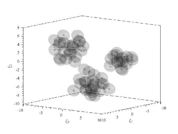
Refer to caption
(a) Data set cover at 200th200^{\textup{th}} time period.
(b) Size of ℙ~n\tilde{\mathbb{P}}^{n} (ℙ^n\hat{\mathbb{P}}^{n}) and count of CP~n(l)\tilde{\rm{CP}}_{n}^{(l)} (CPn(l){\rm{CP}}_{n}^{(l)}) solved with(out) I-Cover Algorithm.
Refer to caption
(c) Relative error of Jnϵ1​(𝒙(r)){J}^{\epsilon_{1}}_{n}(\boldsymbol{x}^{(r)}) over time, with the I-Cover Algorithm.
Refer to caption
(d) Relative error of Jnϵ1​(𝒙(r)){J}^{\epsilon_{1}}_{n}(\boldsymbol{x}^{(r)}) over time, without the I-Cover Algorithm.
(e) Size of ℙ^n\hat{\mathbb{P}}^{n} (ℙ~n\tilde{\mathbb{P}}^{n}) indicated by |Ξn||\Xi_{n}| (|𝒞n||\mathcal{C}_{n}|) and count of CP~n(l)\tilde{\rm{CP}}_{n}^{(l)} solved.
Refer to caption
(f) Relative error of Jnϵ1​(𝒙(r)){J}^{\epsilon_{1}}_{n}(\boldsymbol{x}^{(r)}) over time, with the I-Cover Algorithm.
Fig. 3: Simulation results of the Online Data Assimilation Algorithm, with and without the Incremental Covering Algorithm

To evaluate the quality of the obtained ϵ1\epsilon_{1}-proper data-driven decision with the streaming data, we estimate the optimizer of (P), 𝒙⋆\boldsymbol{x}^{\star}, by minimizing the average value of the cost function ff for a validation data set of Nval=104N_{\textup{val}}=10^{4} data points randomly generated from the distribution ℙ\mathbb{P} (in the simulation case ℙ\mathbb{P} is known). We take the resulting objective value as the estimated optimal objective value for Problem (P), i.e., J⋆:=J⋆​(𝒙⋆)J^{\star}:={J}^{\star}({\boldsymbol{x}}^{\star}). We calculate J⋆​(𝒙⋆){J}^{\star}({\boldsymbol{x}}^{\star}) using the underline distribution ℙ\mathbb{P}, serving as the true but unknown scale to evaluate the goodness of the certificate obtained throughout the algorithm.

Figure 3c and Figure 3d show the evolution of the certificate sequence {Jnϵ1​(𝒙(r))}n=1,r=1N,∞\{{J}_{n}^{\epsilon_{1}}(\boldsymbol{x}^{(r)})\}_{n=1,r=1}^{N,\infty} with the I-Cover Algorithm and that without the I-Cover Algorithm, respectively. Here, the optimal decision of (P) is trivially 𝒙⋆=0{\boldsymbol{x}}^{\star}=0, and for both algorithms the subgradient counterpart of the OnDA Algorithm returns the optimal decision after the first data point ξ1{\xi}_{1} is used. Therefore, after a very short period within the first second, both figures start reflecting the certificate evolution under the decision sequence {𝒙(r)≈0}r=r2∞\{\boldsymbol{x}^{(r)}\approx 0\}_{r=r_{2}}^{\infty}. The gray solid line in both Figure 3c and Figure 3d show the relative goodness of the certificates for the currently used ϵ1\epsilon_{1}-proper data-driven decision 𝒙(r)≈0\boldsymbol{x}^{(r)}\approx 0 calibrated by the estimated optimal value J⋆J^{\star} over time. The black segments on the gray solid line indicate that the C-Gen Algorithm is executing for certificates update, while at these time intervals the old certificate Jnϵ1​(𝒙nϵ2){J}_{n}^{\epsilon_{1}}(\boldsymbol{x}_{n}^{\epsilon_{2}}), associated with the ϵ2\epsilon_{2}-optimal and ϵ1\epsilon_{1}-proper data-driven decision 𝒙nϵ2\boldsymbol{x}_{n}^{\epsilon_{2}}, is still valid to guarantee the performance under the old confidence 1−βn1-\beta_{n}. This situation commonly happens when a new data set Ξn+1{\Xi}_{n+1} is streamed in and a new certificate Jn+1ϵ1​(𝒙(r)){J}_{n+1}^{\epsilon_{1}}(\boldsymbol{x}^{(r)}) is yet to be obtained. It can be seen that after a few samples streamed, both the obtained certificate becomes close (within 10%10\%) to the estimated true optimal value J⋆J^{\star}. In Figure 3d however, as the data streams over 5050 seconds, the computing cost for updating certificates becomes significant for the algorithm without the I-Cover Algorithm. After 100th100^{\textup{th}} data point has been assimilated, the certificate Jnϵ1​(𝒙(r)){J}_{n}^{\epsilon_{1}}(\boldsymbol{x}^{(r)}) stops updating for all n≥100n\geq 100. And, further, after all the data points streamed (in 200200 seconds), the algorithm took about 7070 seconds to terminate the algorithm with certificate J200ϵ1​(𝒙(r)){J}_{200}^{\epsilon_{1}}(\boldsymbol{x}^{(r)}). This is a clear disadvantage compared to the algorithm with the I-Cover Algorithm, which terminates as soon as all the data points were taken in.

IX-B Study 2: OnDA Algorithm with Large Streaming Data Sets

Here, we are to find an ϵ2\epsilon_{2}-optimal, ϵ1\epsilon_{1}-proper decision 𝒙∈30\boldsymbol{x}\in\real^{30} for Problem (P). We consider N=500N=500 iid sample points {ξk}k=1N\{{\xi}_{k}\}_{k=1}^{N} streaming randomly in between every 11 to 33 seconds with each data point ξk∈10{\xi}_{k}\in\real^{10} a realization of ℙ\mathbb{P}. We assume that the unknown distribution is a multivariate Gaussian mixture distribution with three centers where the components of the mean of each center are uniformly chosen between [−10,10][-10,10], and the variance matrix is 𝑰m\boldsymbol{I}_{m} for each center. We assume the cost function f:30×10→f:\real^{30}\times\real^{10}\rightarrow\real to be f⁡(𝒙,ξ):=𝒙⊤​A​𝒙+𝒙⊤​B​ξ+ξ⊤​C​ξf(\boldsymbol{x},\xi):={\boldsymbol{x}}^{\top}A\boldsymbol{x}+{\boldsymbol{x}}^{\top}B\xi+{\xi}^{\top}C\xi with random values for the positive semi-definite matrix A∈30×30A\in\real^{30\times 30}, B∈30×10B\in\real^{30\times 10} and negative definite matrix C∈10×10C\in\real^{10\times 10}. The radius of the Euclidean ball for the I-Cover Algorithm is w=5w=5.

Similarly to Figure 3b, Figure 3e demonstrates the incremental construction of the distribution ℙ~n\tilde{\mathbb{P}}^{n} and the accumulated number of Problem ( ~ P2 n , p ) solved over time. Clearly, after certain amount of data have been assimilated, the structure of the data set was inferred by the I-Cover Algorithm and the number of Euclidean balls used to cover the data set is about 2020. Also, after the 100th100^{\textup{th}} time period (from 100100 to 200200 seconds in this case), the algorithm can validate new certificate without solving any Problem ( ~ P2 n , p ). This feature dramatically improves the performance of the OnDA Algorithm and makes the algorithm flexible for online settings.

Similarly to Figure 3c, Figure 3f shows the evolution of the certificate sequence {Jnϵ1​(𝒙(r))}n=1,r=1N,∞\{{J}_{n}^{\epsilon_{1}}(\boldsymbol{x}^{(r)})\}_{n=1,r=1}^{N,\infty} for the decision sequence {𝒙(r)}r=1∞\{\boldsymbol{x}^{(r)}\}_{r=1}^{\infty}. In the same way as in the last case study, the obtained certificate becomes close to the estimated true optimal value J⋆J^{\star} (within 10%10\%) after about 2525 seconds with the assimilation of 1010 data sets. Also, as more data sets are assimilated, the update of the certificate Jnϵ1​(𝒙nϵ2){J}_{n}^{\epsilon_{1}}(\boldsymbol{x}^{\epsilon_{2}}_{n}) remains fast and the algorithm terminates within a second after the last data set was streamed in.

X Conclusions

In this paper, we have proposed the Online Data Assimilation Algorithm (the OnDA Algorithm) to solve the problem in the form of (P), where the realizations of the unknown distribution (i.e., the streaming data) are collected over time in order for the real-time data-driven decision of (P) to have guaranteed out-of-sample performance. The data-driven decision with the certificate that guarantees out-of-sample performance are available any time during the execution of the algorithm, and the optimal data-driven decision are approached with a (sub)linear convergence rate. The algorithm terminates after collecting a sufficient amount of data to make good decision. To facilitate the decision making, an enhanced version of the proposed algorithm is further constructed, by using an Incremental Covering Algorithm (the I-Cover Algorithm) to estimate new ambiguity sets over time. We provided sample problems and showed the actual performance of the proposed OnDA Algorithm with the I-Cover Algorithm over time. Future work will generalize the results for weaker assumptions of the problem and potentially extend the algorithm to scenarios that include system dynamics.

There are mainly two types of Numerical methods that serve as the main ingredients of our OnDA Algorithm. One type is given by Frank-Wolfe Algorithm (FWA) variants and another is the Subgradient Algorithm. In this Section, we describe FWA and the Away-step Frank-Wolfe Algorithm (AFWA) for the sake of completeness. We combine AFWA with another variant, the Simplicial Algorithm, in Section V. For the Subgradient Algorithm, please refer to [17, 18, 20].

Frank-Wolfe Algorithm over a unit simplex

To solve convex programs over a unit simplex, we introduce the FWA and AFWA following [13, 12]. Let us denote the mm-dimensional unit simplex by Δm:={λ∈m| 1m⊤λ=1,λ≥0}\Delta_{m}:=\{\lambda\in\real^{m}\;|\;{\boldsymbol{1}_{m}}^{\top}\lambda=1,\;\lambda\geq 0\}. Let Λm{\Lambda}_{m} be the set of all extreme points for the simplex Δm\Delta_{m}. Consider the maximization of a concave function f⁡(𝒙)f(\boldsymbol{x}) subject to 𝒙∈Δm\boldsymbol{x}\in\Delta_{m}; we refer to this problem by (⋆)(\star) and denote by 𝒙⋆\boldsymbol{x}^{\star} an optimizer of (⋆)(\star). We call 𝒙ϵ{\boldsymbol{x}}^{\epsilon} an ϵ\epsilon-optimal solution of (⋆)(\star), if 𝒙ϵ∈Δm{\boldsymbol{x}}^{\epsilon}\in\Delta_{m} and f⁡(𝒙⋆)−f⁡(𝒙ϵ)≤ϵf(\boldsymbol{x}^{\star})-f({\boldsymbol{x}}^{\epsilon})\leq\epsilon. The classical FWA solves problem (⋆)(\star) to an 𝒙ϵ{\boldsymbol{x}}^{\epsilon} via the iterative process as follows. Let 𝒙(0)∈Δm\boldsymbol{x}^{(0)}\in\Delta_{m} denote a random initial point for FWA. For each iteration kk with an 𝒙(k)∈Δm\boldsymbol{x}^{(k)}\in\Delta_{m}, the concavity of ff enables f(𝒙⋆)≤f(𝒙(k))+∇f(𝒙(k))⊤(𝒙⋆−𝒙(k))f(\boldsymbol{x}^{\star})\leq f(\boldsymbol{x}^{(k)})+{\nabla f(\boldsymbol{x}^{(k)})}^{\top}(\boldsymbol{x}^{\star}-\boldsymbol{x}^{(k)}), which implies f⁡(𝒙⋆)≤f⁡(𝒙(k))+max𝒙∈Δm⁡∇f​(𝒙(k))⊤​(𝒙−𝒙(k))f(\boldsymbol{x}^{\star})\leq f(\boldsymbol{x}^{(k)})+\max_{\boldsymbol{x}\in\Delta_{m}}{\nabla f(\boldsymbol{x}^{(k)})}^{\top}(\boldsymbol{x}-\boldsymbol{x}^{(k)}). Using this property, we define a FW search point 𝒔(k)\boldsymbol{s}^{(k)} by an extreme point such that 𝒔(k)∈argmax𝒙∈Δm∇f(𝒙(k))⊤(𝒙−𝒙(k))\boldsymbol{s}^{(k)}\in\argmax_{\boldsymbol{x}\in\Delta_{m}}{\nabla f(\boldsymbol{x}^{(k)})}^{\top}(\boldsymbol{x}-\boldsymbol{x}^{(k)}). With this search point we define the FW direction at 𝒙(k)\boldsymbol{x}^{(k)} by dFW(k):=𝒔(k)−𝒙(k)d_{\textup{FW}}^{(k)}:=\boldsymbol{s}^{(k)}-\boldsymbol{x}^{(k)}. The classical FWA then iteratively finds a FW direction and solves a line search problem over this direction until an ϵ{\epsilon}-optimal solution 𝒙ϵ:=𝒙(k){\boldsymbol{x}}^{\epsilon}:=\boldsymbol{x}^{(k)} is found, certified by η(k):=∇f(𝒙(k))⊤dFW(k)≤ϵ\eta^{(k)}:={\nabla f(\boldsymbol{x}^{(k)})}^{\top}d_{\textup{FW}}^{(k)}\leq\epsilon.

It is known that the classical FWA has linear convergence rate if the cost function ff is μ\mu-strongly concave and the optimum is achieved in the relative interior of the feasible set Δm\Delta_{m}. If the optimal solution lies on the boundary of Δm\Delta_{m}, then this algorithm only has a sublinear convergence rate, due to a zig-zagging phenomenon [13]. AFWA is an extension of the FWA that guarantees the linear convergence rate of the problem (⋆)(\star) under some conditions related to the local strong concavity. The main difference between AFWA and the classical FWA is that the latter solves the line-search problem after obtaining a ascent direction by considering all extreme points, while the AFWA chooses a ascend direction that prevents zig-zagging. We summarize the convergence properties of the AFWA here. For complete descriptions of the AFWA, we refer the reader to [13, 21]. The detailed FWA and AFWA are shown in the following Algorithm tables.

Algorithm 4 Classical FWA for (⋆)(\star): FW(𝒙(0),Δm,ϵ)(\boldsymbol{x}^{(0)},\Delta_{m},\epsilon).
1: ϵ\epsilon-optimal 𝒙ϵ\boldsymbol{x}^{\epsilon};
2: Set k←0k\leftarrow 0, η(k)←+∞\eta^{(k)}\leftarrow+\infty;
3: repeat
4:   Pick 𝒔(k)∈argmax𝒙∈Λm∇f(𝒙(k))⊤(𝒙−𝒙(k))\boldsymbol{s}^{(k)}\in\argmax\limits_{\boldsymbol{x}\in{\Lambda}_{m}}{\nabla f(\boldsymbol{x}^{(k)})}^{\top}(\boldsymbol{x}-\boldsymbol{x}^{(k)});
5:   dFW(k)←𝒔(k)−𝒙(k)d_{\textup{FW}}^{(k)}\leftarrow\boldsymbol{s}^{(k)}-\boldsymbol{x}^{(k)};
6:   η(k)←∇f(𝒙(k))⊤dFW(k)\eta^{(k)}\leftarrow{\nabla f(\boldsymbol{x}^{(k)})}^{\top}d_{\textup{FW}}^{(k)};
7:   Pick γ(k)∈argmaxγ∈[0,1]f​(𝒙(k)+γ​dFW(k))\gamma^{(k)}\in\argmax\limits_{\gamma\in[0,1]}f(\boldsymbol{x}^{(k)}+\gamma d_{\textup{FW}}^{(k)});
8:   𝒙(k+1)←𝒙(k)+γ(k)​dFW(k)\boldsymbol{x}^{(k+1)}\leftarrow\boldsymbol{x}^{(k)}+\gamma^{(k)}d_{\textup{FW}}^{(k)};
9:   k←k+1k\leftarrow k+1;
10: until η(k)≤ϵ\eta^{(k)}\leq\epsilon;
11: Return 𝒙(k)\boldsymbol{x}^{(k)}.
Algorithm 5 AFWA for (⋆)(\star): (𝒙ϵ,objϵ)←(\boldsymbol{x}^{\epsilon},{\operatorname{obj}}^{\epsilon})\leftarrow AFW(f⁡(𝒙),Δm,ϵ)(f(\boldsymbol{x}),\Delta_{m},\epsilon).
1: ϵ\epsilon-optimal 𝒙ϵ\boldsymbol{x}^{\epsilon} with objective objϵ{\operatorname{obj}}^{\epsilon};
2: Set k←0k\leftarrow 0, η(k)←+∞\eta^{(k)}\leftarrow+\infty;
3: Pick 𝒙(k)∈Λm\boldsymbol{x}^{(k)}\in{\Lambda}_{m}, IAct(k):={𝒙(k)}I_{\textup{Act}}^{(k)}:=\{\boldsymbol{x}^{(k)}\}, p=|IAct(k)|p=|I_{\textup{Act}}^{(k)}|;
4: Let αv(k)={1/p, if ​𝒗∈IAct(k),0, if ​𝒗∈Λm−IAct(k),\alpha^{(k)}_{v}=\begin{cases}1/p,\textrm{ if }\boldsymbol{v}\in I_{\textup{Act}}^{(k)},\\ 0,\textrm{ if }\boldsymbol{v}\in{\Lambda}_{m}-I_{\textup{Act}}^{(k)},\end{cases}
5: repeat
6:   Pick 𝒔(k)∈argmax𝒙∈Λm∇f(𝒙(k))T(𝒙−𝒙(k))\boldsymbol{s}^{(k)}\in\argmax\limits_{\boldsymbol{x}\in{\Lambda}_{m}}\nabla f(\boldsymbol{x}^{(k)})^{T}(\boldsymbol{x}-\boldsymbol{x}^{(k)});
7:   dFW(k)←𝒔(k)−𝒙(k)d_{\textup{FW}}^{(k)}\leftarrow\boldsymbol{s}^{(k)}-\boldsymbol{x}^{(k)};
8:   Pick 𝒗(k)∈argmin𝒙∈IAct(k)∇f(𝒙(k))T(𝒙−𝒙(k))\boldsymbol{v}^{(k)}\in\argmin\limits_{\boldsymbol{x}\in I_{\textup{Act}}^{(k)}}\nabla f(\boldsymbol{x}^{(k)})^{T}(\boldsymbol{x}-\boldsymbol{x}^{(k)});
9:   dA(k)←𝒙(k)−𝒗(k)d_{\textup{A}}^{(k)}\leftarrow\boldsymbol{x}^{(k)}-\boldsymbol{v}^{(k)}; ⊳\triangleright Away-step direction
10:   if ⟨∇f​(𝒙(k)),dFW(k)⟩≥⟨∇f​(𝒙(k)),dA(k)⟩\left\langle\nabla f(\boldsymbol{x}^{(k)}),d_{\textup{FW}}^{(k)}\right\rangle\geq\left\langle\nabla f(\boldsymbol{x}^{(k)}),d_{\textup{A}}^{(k)}\right\rangle, then
11:    d(k)←dFW(k)d^{(k)}\leftarrow d_{\textup{FW}}^{(k)};
12:    flag ←\leftarrow True, γmax←1\gamma_{\textup{max}}\leftarrow 1;
13:   else⊳\triangleright AFW direction has larger potential ascent
14:    d(k)←dA(k)d^{(k)}\leftarrow d_{\textup{A}}^{(k)};
15:    γmax←α𝒗(k)(k)/(1−α𝒗(k)(k))\gamma_{\textup{max}}\leftarrow\alpha^{(k)}_{\boldsymbol{v}^{(k)}}/(1-\alpha^{(k)}_{\boldsymbol{v}^{(k)}});
16:   end if
17:   Pick γ(k)∈argmaxγ∈[0,γmax]f​(𝒙(k)+γ​d(k))\gamma^{(k)}\in\argmax\limits_{\gamma\in[0,\gamma_{\textup{max}}]}f(\boldsymbol{x}^{(k)}+\gamma d^{(k)});
18:   if flag is True, then
19:    if γ(k)=1\gamma^{(k)}=1, then ⊳\triangleright Hit extreme point
20:      IAct(k+1)←{𝒔(k)}I_{\textup{Act}}^{(k+1)}\leftarrow\{\boldsymbol{s}^{(k)}\};
21:    else
22:      IAct(k+1)←IAct(k)∪{𝒔(k)}I_{\textup{Act}}^{(k+1)}\leftarrow I_{\textup{Act}}^{(k)}\cup\{\boldsymbol{s}^{(k)}\};
23:    end if
24:    α𝒔(k)(k+1)←(1−γ(k))​α𝒔(k)(k)+γ(k)\alpha^{(k+1)}_{\boldsymbol{s}^{(k)}}\leftarrow(1-\gamma^{(k)})\alpha^{(k)}_{\boldsymbol{s}^{(k)}}+\gamma^{(k)};
25:    α𝒗(k+1)←(1−γ(k))​α𝒗(k)\alpha^{(k+1)}_{\boldsymbol{v}}\leftarrow(1-\gamma^{(k)})\alpha^{(k)}_{\boldsymbol{v}}, ∀𝒗∈IAct(k)−{𝒔(k)}\forall\boldsymbol{v}\in I_{\textup{Act}}^{(k)}-\{\boldsymbol{s}^{(k)}\};
26:   else
27:    if γ(k)=γmax\gamma^{(k)}=\gamma_{\textup{max}}, then ⊳\triangleright Hit Δm\Delta_{m} boundary
28:      IAct(k+1)←IAct(k)−{𝒗(k)}I_{\textup{Act}}^{(k+1)}\leftarrow I_{\textup{Act}}^{(k)}-\{\boldsymbol{v}^{(k)}\};
29:    else
30:      IAct(k+1)←IAct(k)I_{\textup{Act}}^{(k+1)}\leftarrow I_{\textup{Act}}^{(k)};
31:    end if
32:    α𝒗(k)(k+1)=(1+γ(k))​α𝒗(k)(k)−γ(k)\alpha^{(k+1)}_{\boldsymbol{v}^{(k)}}=(1+\gamma^{(k)})\alpha^{(k)}_{\boldsymbol{v}^{(k)}}-\gamma^{(k)};
33:    α𝒗(k+1)=(1+γ(k))​α𝒗(k)\alpha^{(k+1)}_{\boldsymbol{v}}=(1+\gamma^{(k)})\alpha^{(k)}_{\boldsymbol{v}}, ∀𝒗∈IAct(k)−{𝒗(k)}\forall\boldsymbol{v}\in I_{\textup{Act}}^{(k)}-\{\boldsymbol{v}^{(k)}\};
34:   end if
35:   𝒙(k+1)←𝒙(k)+γ(k)​d(k)\boldsymbol{x}^{(k+1)}\leftarrow\boldsymbol{x}^{(k)}+\gamma^{(k)}d^{(k)};
36:   k←k+1k\leftarrow k+1;
37: until η(k)≤ϵ\eta^{(k)}\leq\epsilon;
38: Return 𝒙ϵ←𝒙(k)\boldsymbol{x}^{\epsilon}\leftarrow\boldsymbol{x}^{(k)} and objϵ←f⁡(𝒙ϵ){\operatorname{obj}}^{\epsilon}\leftarrow f(\boldsymbol{x}^{\epsilon}).
Theorem .1 (Linear convergence of AFWA [13, Theorem 8]).

Suppose the function ff has a curvature constant CfC_{f} and a geometric strong concavity constant μf\mu_{f} on Δm\Delta_{m}, as defined in footnote 2 Let us define the decay rate κ:=1−μf/(4​Cf)∈(0,1)⊂\kappa:=1-{\mu_{f}}/({4C_{f}})\in(0,1)\subset\real. Then the suboptimality bound at the iteration point 𝐱(k)\boldsymbol{x}^{(k)} of the AFWA decreases geometrically as f⁡(𝐱⋆)−f⁡(𝐱(k+1))≤κ⁡(f⁡(𝐱⋆)−f⁡(𝐱(k)))f(\boldsymbol{x}^{\star})-f(\boldsymbol{x}^{(k+1)})\leq\kappa(f(\boldsymbol{x}^{\star})-f(\boldsymbol{x}^{(k)})).

Proofs

Lemma 5

Proof:

Following [5, 3] and from Theorem IV.1, we prove that Jn​(𝒙){J}_{n}(\boldsymbol{x}) is a valid certificate for (1). Knowing that (4) is obtained by letting the right-hand side of (3) to be equal to a given βn\beta_{n}, for each nn we substitute (4) into the right-hand side of (3), yielding 𝐏n{dW(ℙ,ℙ^n)≥ϵ(βn)}≤βn\mathbf{P}^{n}\{d_{W}(\mathbb{P},\hat{\mathbb{P}}^{n})\geq\epsilon(\beta_{n})\}\leq\beta_{n} for each nn. This means that a data set Ξn{\Xi}_{n} we can construct an empirical probability measure ℙ^n\hat{\mathbb{P}}^{n} such that dW​(ℙ,ℙ^n)≤ϵ⁡(βn)d_{W}(\mathbb{P},\hat{\mathbb{P}}^{n})\leq\epsilon(\beta_{n}) with probability at least 1−βn1-\beta_{n}. Namely, 𝐏n{ℙ∈𝔹ϵ⁡(βn)(ℙ^n)}≥1−βn\mathbf{P}^{n}\{\mathbb{P}\in\mathbb{B}_{\epsilon(\beta_{n})}(\hat{\mathbb{P}}^{n})\}\geq 1-\beta_{n}. Thus, for all 𝒙∈d\boldsymbol{x}\in\real^{d}, we have 𝐏n{ℙ∈𝔹ϵ⁡(βn)(ℙ^n)}=𝐏n{𝔼ℙ[f(𝒙,ξ)]≤supℚ∈𝒫n𝔼ℚ[f(𝒙,ξ)]}=𝐏n{𝔼ℙ[f(𝒙,ξ)]≤Jn(𝒙)}≥1−βn\mathbf{P}^{n}\{\mathbb{P}\in\mathbb{B}_{\epsilon(\beta_{n})}(\hat{\mathbb{P}}^{n})\}=\mathbf{P}^{n}\{\mathbb{E}_{\mathbb{P}}[f(\boldsymbol{x},\xi)]\leq\sup\limits_{\mathbb{Q}\in\mathcal{P}_{n}}{\mathbb{E}_{\mathbb{Q}}[f(\boldsymbol{x},\xi)]}\}=\mathbf{P}^{n}\{\mathbb{E}_{\mathbb{P}}[f(\boldsymbol{x},\xi)]\leq{J}_{n}(\boldsymbol{x})\}\geq 1-\beta_{n}.

Lemma IV.2

In the following, we for matrices A1∈m×dA_{1}\in\real^{m\times d} and A2∈p×qA_{2}\in\real^{p\times q}, we let A1⊕A2A_{1}\oplus A_{2} denote their direct sum. The shorthand notation ⊕i=1mAi\oplus_{i=1}^{m}A_{i} represents A1⊕⋯⊕AmA_{1}\oplus\cdots\oplus A_{m}.

Proof:

To prove 1, for any feasible solution (𝒖~,𝒗~)(\tilde{\boldsymbol{u}},\tilde{\boldsymbol{v}}) of (P2n), we compute 1n​∑k=1n‖𝒚~k‖=1n​∑k=1n‖𝒖~k−𝒗~k‖≤1n​∑k=1n‖𝒖~k‖+1n​∑k=1n‖𝒗~k‖=1n​𝟏m​n⊤​𝒖~+1n​𝟏m​n⊤​𝒗~=1n​𝟏2​m​n⊤​(𝒖~,𝒗~)=ϵ⁡(βn)\frac{1}{n}\sum_{k=1}^{n}\|\tilde{\boldsymbol{y}}_{k}\|=\frac{1}{n}\sum_{k=1}^{n}\|\tilde{\boldsymbol{u}}_{k}-\tilde{\boldsymbol{v}}_{k}\|\leq\frac{1}{n}\sum_{k=1}^{n}\|\tilde{\boldsymbol{u}}_{k}\|+\frac{1}{n}\sum_{k=1}^{n}\|\tilde{\boldsymbol{v}}_{k}\|=\frac{1}{n}{\boldsymbol{1}_{mn}}^{\top}\tilde{\boldsymbol{u}}+\frac{1}{n}{\boldsymbol{1}_{mn}}^{\top}\tilde{\boldsymbol{v}}=\frac{1}{n}{\boldsymbol{1}_{2mn}}^{\top}(\tilde{\boldsymbol{u}},\tilde{\boldsymbol{v}})=\epsilon(\beta_{n}). Therefore (𝒚~1,…,𝒚~n)(\tilde{\boldsymbol{y}}_{1},\ldots,\tilde{\boldsymbol{y}}_{n}) is feasible for (P1n).

For 2, we exploit that any feasible solution 𝒚~\tilde{\boldsymbol{y}} of (P1n) is a linear combination of the extreme points of the constraint set in (P1n). Let us denote the matrix An:=[⊕i=1nIm,−⊕i=1nIm]∈m​n×2​m​nA_{n}:=[\oplus_{i=1}^{n}I_{m},-\oplus_{i=1}^{n}I_{m}]\in\real^{mn\times 2mn}. By construction of Problem (P2n), we see that each column vector of the matrix n​ϵ​(βn)​Ann\epsilon(\beta_{n})A_{n} is a concatenated vector of an extreme point of Problem (P1n), and that all the extreme points of (P1n) are included. Then, any feasible solution of (P1n) can be written as 𝒚~=n​ϵ​(βn)​An​(𝒖^,𝒗^)\tilde{\boldsymbol{y}}=n\epsilon(\beta_{n})A_{n}(\hat{\boldsymbol{u}},\hat{\boldsymbol{v}}) where (𝒖^,𝒗^)(\hat{\boldsymbol{u}},\hat{\boldsymbol{v}}) is a vector of the convex combination coefficients of the extreme points of the constraint set in (P1n). Clearly, we have (𝒖^,𝒗^)∈Δ2​m​n(\hat{\boldsymbol{u}},\hat{\boldsymbol{v}})\in\Delta_{2mn}, i.e., n​ϵ​(βn)​(𝒖^,𝒗^)n\epsilon(\beta_{n})(\hat{\boldsymbol{u}},\hat{\boldsymbol{v}}) is in the feasible set of the Problem (P2n). Then, by construction (𝒖~,𝒗~):=n​ϵ​(βn)​(𝒖^,𝒗^)(\tilde{\boldsymbol{u}},\tilde{\boldsymbol{v}}):=n\epsilon(\beta_{n})(\hat{\boldsymbol{u}},\hat{\boldsymbol{v}}) is feasible for (P2n).

For 3, since (P1n) and (P2n) are the same in the sense of (1) and (2), then if (𝒖~⋆,𝒗~⋆)(\tilde{\boldsymbol{u}}^{\star},\tilde{\boldsymbol{v}}^{\star}) is an optimizer of (P2n), by letting 𝒚~k⋆:=𝒖~k⋆−𝒗~k⋆\tilde{\boldsymbol{y}}_{k}^{\star}:=\tilde{\boldsymbol{u}}_{k}^{\star}-\tilde{\boldsymbol{v}}_{k}^{\star} for each k∈{1,…,n}k\in\{1,\dots,n\} we know the objective values of the two problems coincide. We claim that the optimum of (P1n) is achieved via the optimizer 𝒚~⋆\tilde{\boldsymbol{y}}^{\star}. If not, then there exists 𝒚^⋆≠𝒚~⋆\hat{\boldsymbol{y}}^{\star}\neq\tilde{\boldsymbol{y}}^{\star} such that the optimum is achieved with higher value. Then, from the construction in (2) we can find a feasible solution (𝒖^,𝒗^)(\hat{\boldsymbol{u}},\hat{\boldsymbol{v}}) of (P2n) that results in a higher objective value. This contradicts the assumption that (𝒖~⋆,𝒗~⋆)(\tilde{\boldsymbol{u}}^{\star},\tilde{\boldsymbol{v}}^{\star}) is an optimizer of (P2n).

Theorem V.1

Proof:

Given tolerance ϵ1\epsilon_{1}, decision 𝒙\boldsymbol{x} and any data set Ξn{\Xi}_{n} with n∈{1,…,N}n\in\{1,\dots,N\}, let Hn:m​n→H_{n}:\real^{mn}\rightarrow\real, Hn:=1n​∑k=1nhkH_{n}:=\frac{1}{n}\sum_{k=1}^{n}h_{k} denote the objective function of (P2n) and let 𝒮n\mathcal{S}_{n} denote the family of subsets of Λ2​m​n\Lambda_{2mn}. In the procedure of C-Gen Algorithm, let us consider a sequence of generated candidate vertex sets: In(l)⊂In(l+1)I_{n}^{(l)}\subset I_{n}^{(l+1)}, l=0,1,2,…l=0,1,2,\ldots with In(l)∈𝒮nI_{n}^{(l)}\in\mathcal{S}_{n}. We show the convergence of C-Gen Algorithm for any data set Ξn{\Xi}_{n}, by two steps.

Step 1) The sequence {In(l)}l\{I_{n}^{(l)}\}_{l} is finite and the number of iterations is at most 2​m​n2mn. For each ll and candidate optimizer 𝒚(l−1)\boldsymbol{y}^{(l-1)}, we generate a nonempty set of search points Ω(l)\Omega^{(l)} with suboptimality gap η(l)\eta^{(l)} via (LP n ( l ) ). If η(l)≤ϵ1\eta^{(l)}\leq\epsilon_{1}, then we solved (P2n) to ϵ1\epsilon_{1}-optimality and ll is therefore finite, otherwise we update In(l):=In(l−1)∪Ω(l)I_{n}^{(l)}:=I_{n}^{(l-1)}\cup\Omega^{(l)}. Given that the maximal cardinality of each In(l)∈𝒮nI_{n}^{(l)}\in\mathcal{S}_{n} is bounded by 2​m​n2mn, then it is sufficient to show Ω(l)∩In(l−1)=Ø\Omega^{(l)}\cap I_{n}^{(l-1)}=\O. Because 𝒚(l−1)\boldsymbol{y}^{(l-1)} is an ϵ1\epsilon_{1}-optimal of (CP n ( l ) ) under conv⁡(In(l−1)){\operatorname{conv}}(I_{n}^{(l-1)}), then for any 𝒚∈conv⁡(In(l−1)){\boldsymbol{y}}\in{\operatorname{conv}}(I_{n}^{(l-1)}), it holds that 1n​∑k=1n⟨∇hk​(𝒚k(l−1)),𝒚k−𝒚k(l−1)⟩≤ϵ1\frac{1}{n}\sum_{k=1}^{n}\langle\nabla h_{k}(\boldsymbol{y}^{(l-1)}_{k}),\boldsymbol{y}_{k}-\boldsymbol{y}^{(l-1)}_{k}\rangle\leq\epsilon_{1}. Since any element in Ω(l)\Omega^{(l)} is such that η(l)>ϵ1\eta^{(l)}>\epsilon_{1}, then for any 𝒚∈conv⁡(In(l−1)){\boldsymbol{y}}\in{\operatorname{conv}}(I_{n}^{(l-1)}), we have 𝒚∉Ω(l){\boldsymbol{y}}\notin\Omega^{(l)}, which concludes Ω(l)∩In(l−1)=Ø\Omega^{(l)}\cap I_{n}^{(l-1)}=\O. Further, the cardinality of Ω(l)\Omega^{(l)} is at least one for every iteration ll, then after at most 2​m​n2mn steps the cardinality of In(l)I_{n}^{(l)} becomes 2​m​n2mn, which implies the ϵ1\epsilon_{1}-optimality of (P2n) by the ϵ1\epsilon_{1}-optimality of (CP n ( l ) ).

Step 2) The computational bound of C-Gen Algorithm is quantified. To see this, consider the problems {(LP n ( l ) )}l\{\eqref{eq:LP}\}_{l} and {(CP n ( l ) )}l\{\eqref{eq:CP}\}_{l}. By Assumption V.2 on the cheap access of the gradients, the computation of (LP n ( l ) ) is negligible. Thus, the computational bound is given by the sum of the steps to solve the {(CP n ( l ) )}l\{\eqref{eq:CP}\}_{l}, where the number of iterations ll is 2​m​n2mn in the worst case.

For each (CP n ( l ) ) solved by AFWA, index the AFWA iterations by i=0,1,2,…i=0,1,2,\ldots, let obji(l){\operatorname{obj}}_{i}^{(l)} be the objective value at each iteration, and assume the optimal objective value is obj⋆(l){\operatorname{obj}}_{\star}^{(l)}. As in Theorem .1, let κn,l∈(0,1)⊂\kappa_{{{n}},l}\in(0,1)\subset\real be the decay parameter related to local strong concavity of HnH_{n} over conv⁡(In(l))\operatorname{conv}(I_{n}^{(l)}). Then using the linear convergence rate of the AFWA, each (CP n ( l ) ) achieves the following computational bound

obj⋆(l)−obji(l)≤κn,li​(obj⋆(l)−obj0(l)),{\operatorname{obj}}_{\star}^{(l)}-{\operatorname{obj}}_{i}^{(l)}\leq\kappa_{{{n}},l}^{i}({\operatorname{obj}}_{\star}^{(l)}-{\operatorname{obj}}_{0}^{(l)}),

where the initial condition obj0(l){\operatorname{obj}}_{0}^{(l)} results from an ϵ1\epsilon_{1}-optimal optimizer of CP at iteration l−1l-1, i.e., we can equivalently denote obj0(l){\operatorname{obj}}_{0}^{(l)} by Jn(l−1)​(𝒙){J}_{n}^{(l-1)}(\boldsymbol{x}), for all l∈{1,…,2​m​n}l\in\{1,\dots,2mn\}.

Let us consider sequence {(CP n ( l ) )}l\{\eqref{eq:CP}\}_{l} with feasible sets {conv⁡(In(l))}l\{\operatorname{conv}(I_{n}^{(l)})\}_{l}. Then we have

conv⁡(In(0))⊂conv⁡(In(1))⊂⋯⊂conv⁡(In(2​m​n))\operatorname{conv}(I_{n}^{(0)})\subset\operatorname{conv}(I_{n}^{(1)})\subset\cdots\subset\operatorname{conv}(I_{n}^{(2mn)}).

This results into monotonically decaying parameters and (ϵ1\epsilon_{1}-)optimal objective values, as given in the following

0<κn,1≤κn,2≤⋯≤κn,2​m​n<10<\kappa_{{{n}},1}\leq\kappa_{{{n}},2}\leq\cdots\leq\kappa_{{{n}},2mn}<1,

Jn(0)​(𝒙)≤Jn(1)​(𝒙)≤⋯≤Jn(2​m​n)​(𝒙){J}_{n}^{(0)}(\boldsymbol{x})\leq{J}_{n}^{(1)}(\boldsymbol{x})\leq\cdots\leq{J}_{n}^{(2mn)}(\boldsymbol{x}),

obj⋆(0)≤obj⋆(1)≤⋯≤obj⋆(2​m​n){\operatorname{obj}}^{(0)}_{\star}\leq{\operatorname{obj}}_{\star}^{(1)}\leq\cdots\leq{\operatorname{obj}}_{\star}^{(2mn)}.

Using the previous notation, we can identify Jn(2​m​n)​(𝒙)≡Jnϵ1​(𝒙){J}_{n}^{(2mn)}(\boldsymbol{x})\equiv{J}_{n}^{\epsilon_{1}}(\boldsymbol{x}), obj⋆(0)≡Jn(0)​(𝒙){\operatorname{obj}}^{(0)}_{\star}\equiv{J}_{n}^{(0)}(\boldsymbol{x}), and obj⋆(2​m​n)≡Jn​(𝒙){\operatorname{obj}}_{\star}^{(2mn)}\equiv{J}_{n}(\boldsymbol{x}). Let us denote κ:=maxn,l⁡{κn,l}\kappa:=\max_{{{n}},l}\{\kappa_{{{n}},l}\}. Then, by solving each (CP n ( l ) ) to ϵ1\epsilon_{1}-optimality, it leads to the accumulated computational steps ϕ⁡(n):=∑lil\phi(n):=\sum_{l}i_{l}, where each ili_{l} is the computation step for ϵ1\epsilon_{1}-optimal (CP n ( l ) ) that satisfies the following inequality

κil​(Jn​(𝒙)−Jn(0)​(𝒙))≤ϵ1,l∈{1,…,2​m​n}.\kappa^{i_{l}}({J}_{n}(\boldsymbol{x})-{J}_{n}^{(0)}(\boldsymbol{x}))\leq\epsilon_{1},\quad l\in\{1,\dots,2mn\}.

Finally, in the worst-case scenario, the computational bound of the C-Gen Algorithm is

ϕ⁡(n)≤(2​m​n)​logκ⁡(ϵ1Jn​(𝒙)−Jn(0)​(𝒙)).\phi(n)\leq(2mn){\log}_{\kappa}(\frac{\epsilon_{1}}{{J}_{n}(\boldsymbol{x})-{J}_{n}^{(0)}(\boldsymbol{x})}).

Next, we show the convergence of the C-Gen Algorithm under online data sets {Ξn}n=1N\{{\Xi}_{n}\}_{n=1}^{N}. Similarly to the proof for the computational bound for a given nn, we can compute the worst-case bound under {Ξn}n=1N\{{\Xi}_{n}\}_{n=1}^{N}, by summing over the steps required to solve the {(CP n ( l ) )}n,l\{\eqref{eq:CP}\}_{n,l}. This leads to the stated bound ϕ¯​(n)\bar{\phi}(n), where the empirical cost JNsae​(𝒙)J^{\textup{sae}}_{N}(\boldsymbol{x}) serves as the cost of initial condition 𝒚(0):=𝟎2​m​N\boldsymbol{y}^{(0)}:=\boldsymbol{0}_{2mN}. In this way, when the data-streaming rate is slower or equal than (ϕ¯​(1))−1(\bar{\phi}(1))^{-1}, we claim that C-Gen Algorithm can always find the certificate for each data set Ξn{\Xi}_{n}. This is because in each time period nn, we only have 2​m​n2mn extreme points, and 2​m​(n−1)2m(n-1) has been explored due to the adaptation of the candidate vertex set In(0)I_{n}^{(0)}.

Lemma VI.1

Proof:

For any 𝒙\boldsymbol{x}, 𝒚∈d\boldsymbol{y}\in\real^{d} and t∈[0,1]⊂t\in[0,1]\subset\real, we have 𝒛=t𝒙+(1−t)𝒚∈d\boldsymbol{z}=t\boldsymbol{x}+(1-t)\boldsymbol{y}\in\real^{d} and an optimizer of (5), ℚn⋆​(𝒛)\mathbb{Q}_{n}^{\star}(\boldsymbol{z}), such that

Jn​(𝒛)≤𝔼ℚn⋆​(𝒛)​[t​f​(𝒙,ξ)+(1−t)​f​(𝒚,ξ)]=t​𝔼ℚn⋆​(𝒛)​[f⁡(𝒙,ξ)]+(1−t)​𝔼ℚn⋆​(𝒛)​[f⁡(𝒚,ξ)]≤t​Jn​(𝒙)+(1−t)​Jn​(𝒚).\begin{split}{J}_{n}(\boldsymbol{z})\leq&{\mathbb{E}_{\mathbb{Q}_{n}^{\star}(\boldsymbol{z})}[tf(\boldsymbol{x},\xi)+(1-t)f(\boldsymbol{y},\xi)]}\\ =&t{\mathbb{E}_{\mathbb{Q}_{n}^{\star}(\boldsymbol{z})}[f(\boldsymbol{x},\xi)]+(1-t)\mathbb{E}_{\mathbb{Q}_{n}^{\star}(\boldsymbol{z})}[f(\boldsymbol{y},\xi)]}\\ \leq&t{J}_{n}(\boldsymbol{x})+(1-t){J}_{n}(\boldsymbol{y}).\end{split}

Lemma VI.2

Proof:

Let us consider the function 𝔼ℚnϵ1​(𝒙(r))​[f​(𝒙,ξ)]{\mathbb{E}_{\mathbb{Q}_{n}^{\epsilon_{1}}(\boldsymbol{x}^{(r)})}[f(\boldsymbol{x},\xi)]}. Using Assumption VI.1 on convexity of ff in 𝒙\boldsymbol{x}, we have for any 𝒛∈dom⁡Jn\boldsymbol{z}\in{\operatorname{dom}}\>{J}_{n} the following relation

𝔼ℚnϵ1​(𝒙(r))​[f⁡(𝒛,ξ)]≥Jnϵ1​(𝒙(r))+gnr​(𝒙(r))⊤​(𝒛−𝒙(r)).{\mathbb{E}_{\mathbb{Q}_{n}^{\epsilon_{1}}(\boldsymbol{x}^{(r)})}[f(\boldsymbol{z},\xi)]}\geq{J}_{n}^{\epsilon_{1}}(\boldsymbol{x}^{(r)})+{g_{n}^{r}(\boldsymbol{x}^{(r)})}^{\top}(\boldsymbol{z}-\boldsymbol{x}^{(r)}).

Knowing that Jnϵ1​(𝒙(r))≥Jn​(𝒙(r))−ϵ1{J}_{n}^{\epsilon_{1}}(\boldsymbol{x}^{(r)})\geq{J}_{n}(\boldsymbol{x}^{(r)})-\epsilon_{1} and Jn​(𝒛)≥𝔼ℚnϵ1​(𝒙(r))​[f⁡(𝒛,ξ)]{J}_{n}(\boldsymbol{z})\geq{\mathbb{E}_{\mathbb{Q}_{n}^{\epsilon_{1}}(\boldsymbol{x}^{(r)})}[f(\boldsymbol{z},\xi)]}, this concludes the first part of the proof.

To show the second part, similarly, we also have for any 𝒙~\tilde{\boldsymbol{x}}, 𝒛∈dom⁡Jn\boldsymbol{z}\in{\operatorname{dom}}\>{J}_{n} the following relation

𝔼ℚnϵ1​(𝒙(r))​[f⁡(𝒛,ξ)]≥𝔼ℚnϵ1​(𝒙(r))​[f⁡(𝒙~,ξ)]+gnr​(𝒙~)⊤​(𝒛−𝒙~).{\mathbb{E}_{\mathbb{Q}_{n}^{\epsilon_{1}}(\boldsymbol{x}^{(r)})}[f(\boldsymbol{z},\xi)]}\geq{\mathbb{E}_{\mathbb{Q}_{n}^{\epsilon_{1}}(\boldsymbol{x}^{(r)})}[f(\tilde{\boldsymbol{x}},\xi)]}+{g_{n}^{r}(\tilde{\boldsymbol{x}})}^{\top}(\boldsymbol{z}-\tilde{\boldsymbol{x}}).

Using Point Search Algorithm, we achieve an η>0\eta>0 such that 𝔼ℚnϵ1​(𝒙(r))​[f⁡(𝒙~,ξ)]≥Jn​(𝒙~)−η{\mathbb{E}_{\mathbb{Q}_{n}^{\epsilon_{1}}(\boldsymbol{x}^{(r)})}[f(\tilde{\boldsymbol{x}},\xi)]}\geq{J}_{n}(\tilde{\boldsymbol{x}})-\eta. Finally, by similar statement as in the first part, we claim gnr​(𝒙~)∈∂ϵJn​(𝒙~)g_{n}^{r}(\tilde{\boldsymbol{x}})\in\partial_{\epsilon}{J}_{n}(\tilde{\boldsymbol{x}}).

Lemma VI.3

Proof:

In the nthn^{\textup{th}} time period, let us consider subgradient iterates ii for all rn≤i≤rr_{n}\leq i\leq r

‖𝒙(i+1)−𝒙n⋆‖2=‖𝒙(i)−𝒙n⋆−α(i)​gni​(𝒙(i))max⁡{‖gni​(𝒙(i))‖, 1}‖2=‖𝒙(i)−𝒙n⋆‖2+(α(i))2​min⁡{‖gni​(𝒙(i))‖2,1}−2​α(i)​gni​(𝒙(i))⊤​(𝒙(i)−𝒙n⋆)max⁡{‖gni​(𝒙(i))‖, 1}.\begin{split}&\|\boldsymbol{x}^{(i+1)}-\boldsymbol{x}_{n}^{\star}\|^{2}=\|\boldsymbol{x}^{(i)}-\boldsymbol{x}_{n}^{\star}-\alpha^{(i)}\frac{g_{n}^{i}(\boldsymbol{x}^{(i)})}{\max\{\|g_{n}^{i}(\boldsymbol{x}^{(i)})\|\;,\;1\}}\|^{2}\\ &=\|\boldsymbol{x}^{(i)}-\boldsymbol{x}_{n}^{\star}\|^{2}+(\alpha^{(i)})^{2}\min\{\|g_{n}^{i}(\boldsymbol{x}^{(i)})\|^{2},1\}\\ &\qquad-2\alpha^{(i)}\frac{{g_{n}^{i}(\boldsymbol{x}^{(i)})}^{\top}(\boldsymbol{x}^{(i)}-\boldsymbol{x}_{n}^{\star})}{\max\{\|g_{n}^{i}(\boldsymbol{x}^{(i)})\|\;,\;1\}}.\end{split}

From Lemma VI.2, we know that Jn​(𝒙n⋆)≥Jn​(𝒙(i))+gni​(𝒙(i))⊤​(𝒙n⋆−𝒙(i))−ϵSA{J}_{n}(\boldsymbol{x}_{n}^{\star})\geq{J}_{n}(\boldsymbol{x}^{(i)})+{g_{n}^{i}(\boldsymbol{x}^{(i)})}^{\top}(\boldsymbol{x}_{n}^{\star}-\boldsymbol{x}^{(i)})-\epsilon_{\textup{SA}} for all 𝒙(i)\boldsymbol{x}^{(i)}. Then, we have

‖𝒙(i+1)−𝒙n⋆‖2≤(α(i))2​min⁡{‖gni​(𝒙(i))‖2,1}+‖𝒙(i)−𝒙n⋆‖2+2​α(i)​(Jn​(𝒙n⋆)−Jn​(𝒙(i))+ϵSA)max⁡{‖gni​(𝒙(i))‖, 1}.\begin{split}&\|\boldsymbol{x}^{(i+1)}-\boldsymbol{x}_{n}^{\star}\|^{2}\leq(\alpha^{(i)})^{2}\min\{\|g_{n}^{i}(\boldsymbol{x}^{(i)})\|^{2},1\}\\ &+\|\boldsymbol{x}^{(i)}-\boldsymbol{x}_{n}^{\star}\|^{2}+\frac{2\alpha^{(i)}({J}_{n}(\boldsymbol{x}_{n}^{\star})-{J}_{n}(\boldsymbol{x}^{(i)})+\epsilon_{\textup{SA}})}{\max\{\|g_{n}^{i}(\boldsymbol{x}^{(i)})\|\;,\;1\}}.\end{split}

Combining the inequalities over iterations from rnr_{n} to rr gives

0≤‖𝒙(rn)−𝒙n⋆‖2+∑i=rnr(α(i))2​min⁡{‖gnr​(𝒙(i))‖2, 1}+∑i=rnr2​α(i)​(Jn​(𝒙n⋆)−Jn​(𝒙(i))+ϵSA)max⁡{‖gnr​(𝒙(i))‖, 1}≤‖𝒙(rn)−𝒙n⋆‖2+2​ϵSA​∑i=rnrα(i)+∑i=rnr(α(i))2+∑i=rnr2​α(i)​(Jn​(𝒙n⋆)−Jn​(𝒙(i)))max⁡{‖gnr​(𝒙(i))‖, 1}.\begin{split}&0\leq\|\boldsymbol{x}^{(r_{n})}-\boldsymbol{x}_{n}^{\star}\|^{2}+\sum_{i=r_{n}}^{r}{(\alpha^{(i)})^{2}\min\{\|g_{n}^{r}(\boldsymbol{x}^{(i)})\|^{2}\;,\;1\}}\\ &+\sum_{i=r_{n}}^{r}{\frac{2\alpha^{(i)}({J}_{n}(\boldsymbol{x}_{n}^{\star})-{J}_{n}(\boldsymbol{x}^{(i)})+\epsilon_{\textup{SA}})}{\max\{\|g_{n}^{r}(\boldsymbol{x}^{(i)})\|\;,\;1\}}}\\ &\leq\|\boldsymbol{x}^{(r_{n})}-\boldsymbol{x}_{n}^{\star}\|^{2}+2\epsilon_{\textup{SA}}\sum_{i=r_{n}}^{r}{\alpha^{(i)}}+\sum_{i=r_{n}}^{r}{(\alpha^{(i)})^{2}}\\ &+\sum_{i=r_{n}}^{r}{\frac{2\alpha^{(i)}({J}_{n}(\boldsymbol{x}_{n}^{\star})-{J}_{n}(\boldsymbol{x}^{(i)}))}{\max\{\|g_{n}^{r}(\boldsymbol{x}^{(i)})\|\;,\;1\}}}.\end{split}

Then, using the fact that

∑i=rnr2​α(i)​(Jn​(𝒙n⋆)−Jn​(𝒙(i)))max⁡{‖gnr​(𝒙(i))‖, 1}≤∑i=rnr−2​α(i)​mink∈{rn,…,r}​{Jn​(𝒙(k))−Jn​(𝒙n⋆)}max⁡{‖gnr​(𝒙(i))‖, 1}≤−2​(∑i=rnrα(i))​mink∈{rn,…,r}⁡{Jn​(𝒙(k))}−Jn​(𝒙n⋆)μ,\begin{split}&\sum_{i=r_{n}}^{r}{\frac{2\alpha^{(i)}({J}_{n}(\boldsymbol{x}_{n}^{\star})-{J}_{n}(\boldsymbol{x}^{(i)}))}{\max\{\|g_{n}^{r}(\boldsymbol{x}^{(i)})\|\;,\;1\}}}\leq\\ &\sum_{i=r_{n}}^{r}{\frac{-2\alpha^{(i)}\min\limits_{k\in\{{r_{n}},\dots,{r}\}}\{{J}_{n}(\boldsymbol{x}^{(k)})-{J}_{n}(\boldsymbol{x}_{n}^{\star})\}}{\max\{\|g_{n}^{r}(\boldsymbol{x}^{(i)})\|\;,\;1\}}}\leq\\ &-2(\sum_{i=r_{n}}^{r}{\alpha^{(i)}})\frac{\min\limits_{k\in\{{r_{n}},\dots,{r}\}}\{{J}_{n}(\boldsymbol{x}^{(k)})\}-{J}_{n}(\boldsymbol{x}_{n}^{\star})}{\mu},\end{split}

and the previous iteration, we have

mink∈{rn,…,r}⁡{Jn​(𝒙(k))}−Jn​(𝒙n⋆)≤μ​‖𝒙(rn)−𝒙n⋆‖2+μ​∑i=rnr(α(i))22​(∑i=rnrα(i))+μ​ϵSA.\begin{split}&\min\limits_{k\in\{{r_{n}},\dots,{r}\}}\{{J}_{n}(\boldsymbol{x}^{(k)})\}-{J}_{n}(\boldsymbol{x}_{n}^{\star})\leq\\ &\frac{\mu\|\boldsymbol{x}^{(r_{n})}-\boldsymbol{x}_{n}^{\star}\|^{2}+\mu\sum_{i=r_{n}}^{r}{(\alpha^{(i)})^{2}}}{2(\sum_{i=r_{n}}^{r}{\alpha^{(i)}})}+\mu\epsilon_{\textup{SA}}.\end{split}

Next, it remains to select a step-size rule {α(i)}i=rnr\{\alpha^{(i)}\}_{i=r_{n}}^{r} such that 1) the above right hand side term is upper bounded by ϵ2\epsilon_{2}, and 2) the number of subgradient iterations r¯\bar{r} as described in the lemma is bounded. Note that the selection procedure is not unique, so we propose two step-size rules to obtain an explicit expression of r¯\bar{r}.

For any data set Ξn\Xi_{n}, let us select a sufficiently large value MM to be the diameter of the decision domain of interest, i.e.,

‖𝒙(rn)−𝒙n⋆‖≤M,∀n∈{1,…,N}.\|\boldsymbol{x}^{(r_{n})}-\boldsymbol{x}_{n}^{\star}\|\leq M,\;\forall\,n\in\{1,\dots,N\}.

Then the step size rule and r¯\bar{r} has to satisfy the following

M2+∑i=rnr¯+rn(α(i))22​(∑i=rnr¯+rnα(i))+ϵSA<ϵ2μ.\frac{M^{2}+\sum_{i=r_{n}}^{\bar{r}+r_{n}}{(\alpha^{(i)})^{2}}}{2(\sum_{i=r_{n}}^{\bar{r}+r_{n}}{\alpha^{(i)}})}+\epsilon_{\textup{SA}}<\frac{\epsilon_{2}}{\mu}. (13)

We first consider a constant step-size rule, and select the step size as follows

α(i):=Mr¯+1,∀i∈{rn,…,r¯+rn}.\alpha^{(i)}:=\frac{M}{\sqrt{\bar{r}+1}},\;\forall i\in\{{r_{n}},\dots,{\bar{r}+r_{n}}\}.

Then, to satisfy (13), we determine

r¯:=M2​(ϵ2μ−ϵSA)−2.\bar{r}:=M^{2}\left(\frac{\epsilon_{2}}{\mu}-\epsilon_{\textup{SA}}\right)^{-2}.

Alternatively, consider the divergent but square-summable step-size rule, i.e. ∑i=rn∞α(i)=∞\sum_{i=r_{n}}^{\infty}{\alpha^{(i)}}=\infty, ∑i=rn∞(α(i))2<∞\sum_{i=r_{n}}^{\infty}{(\alpha^{(i)})^{2}}<\infty. For this class of step-size rules, as r¯\bar{r} increases to ∞\infty, we have the left-hand side term of (13) goes to μ​ϵSA<ϵ2\mu\epsilon_{\textup{SA}}<\epsilon_{2}, then there exists a large enough but finite number r¯\bar{r}, such that (13) holds. To see this explicitly, we select the step-size rule to be the harmonic sequence as follows

α(i):=Mi−rn+1,∀i∈{rn,…,r¯+rn}.\alpha^{(i)}:=\frac{M}{i-r_{n}+1},\;\forall i\in\{{r_{n}},\dots,{\bar{r}+r_{n}}\}.

Now we upper bound the numerator and lower bound the denominator of (13) using the following fact

∑i=1r¯+11i2≤2−1r¯+1,∑i=1r¯+11i≥ln⁡(r¯+1).\sum\limits_{i=1}^{\bar{r}+1}\frac{1}{i^{2}}\leq 2-\frac{1}{\bar{r}+1},\quad\sum\limits_{i=1}^{\bar{r}+1}\frac{1}{i}\geq\ln(\bar{r}+1).

Then we determine r¯\bar{r} to be the following

r¯=min⁡{r∈ℕ|M⁡(3−1r+1)≤2​(ϵ2μ−ϵSA)​ln⁡(r+1)}.\bar{r}=\min\{r\in\mathbb{N}\;|\;M(3-\frac{1}{r+1})\leq 2(\frac{\epsilon_{2}}{\mu}-\epsilon_{\textup{SA}})\ln(r+1)\}.

This concludes the proof.

Theorem VI.1

Proof:

The computational bound to achieve an 𝒙nϵ2\boldsymbol{x}_{n}^{\epsilon_{2}} strongly depends on the subgradient iterations r¯:=rn+1−rn\bar{r}:=r_{n+1}-r_{n} in Lemma VI.3 and the number of subgradient functions {gnr}r=rnrn+1\{g_{n}^{r}\}_{r=r_{n}}^{r_{n+1}} constructed via the C-Gen Algorithm. To characterize this bound, we quantify the computational steps for {gnr}r=rnrn+1\{g_{n}^{r}\}_{r=r_{n}}^{r_{n+1}} next.

For each time period nn, let us assume the C-Gen Algorithm has explored the feasible set of (P2n) when obtaining the initial certificate Jnϵ1​(𝒙(rn)){J}_{n}^{\epsilon_{1}}(\boldsymbol{x}^{(r_{n})}). This procedure consumes a worst-case computational time ϕ⁡(n)\phi(n), (or ϕ¯​(1)\bar{\phi}(1) if a data-streaming scenario), as stated in Theorem V.1. After this initial step, every time the Subgradient Algorithm needs to execute C-Gen Algorithm at some r≤rn+1r\leq r_{n+1}, C-Gen Algorithm will solve a unique (CP n ( l ) ) and return ℚnϵ1\mathbb{Q}_{n}^{\epsilon_{1}} for an ϵ1{\epsilon}_{1}-subgradient function gnrg_{n}^{r} at 𝒙(r)\boldsymbol{x}^{(r)}. Let CPr{\textrm{CP}}_{r} denote the unique (CP n ( l ) ) solved at 𝒙(r)\boldsymbol{x}^{(r)}. Then, to quantify the computational steps for {gnr}r=rnrn+1\{g_{n}^{r}\}_{r=r_{n}}^{r_{n+1}}, we compute the sum of the steps to solve {CPr}r\{{\textrm{CP}}_{r}\}_{r}.

Let us denote the number of steps solving CPr{\textrm{CP}}_{r} by iri_{r}, for all r∈{rn,…,rn+1}r\in\{r_{n},\ldots,r_{n+1}\}. Then, we aim to quantify ir+1i_{r+1} for gnr+1g_{n}^{r+1}. To achieve this, let us assume a subgradient function gnrg_{n}^{r} is computed at an iteration rr. Then we perform a subgradient iteration (7) and obtain an 𝒙(r+1)\boldsymbol{x}^{(r+1)}. By using a subgradient estimation strategy, we obtain the optimality gap η(1)\eta^{(1)} via Point Search Algorithm, denoted by η¯r+1:=η(1)\bar{\eta}_{r+1}:=\eta^{(1)}. This gap η¯r+1\bar{\eta}_{r+1} enables us to quantify the distance between the initial objective value and the optimal objective value of CPr+1{\textrm{CP}}_{r+1}. When η¯r+1≤ϵSA\bar{\eta}_{r+1}\leq\epsilon_{\textup{SA}}, the algorithm uses the estimated subgradient function and ir+1=0i_{r+1}=0. Otherwise, the computational steps can be calculated via convergence of AFWA for CPr+1{\textrm{CP}}_{r+1}, by κir+1​η¯r+1≤ϵ1,\kappa^{i_{r+1}}\bar{\eta}_{r+1}\leq\epsilon_{1}, where κ\kappa, or using κ¯\bar{\kappa} for the data-streaming case, is determined as in Theorem V.1. Let us consider a threshold value trt_{r}

tr:={ϵ1,if​η¯r≤ϵSA,η¯r,o.w.t_{r}:=\left\{{\begin{array}[]{*{20}{l}}\epsilon_{1},&\textrm{if}\;\bar{\eta}_{r}\leq\epsilon_{\textup{SA}},\\ \bar{\eta}_{r},&\textrm{o.w.}\end{array}}\right.

Then we can represent each value iri_{r} by ir=logκ⁡(ϵ1tr),r∈{rn,…,rn+1}.i_{r}={\log}_{\kappa}(\frac{\epsilon_{1}}{t_{r}}),\;r\in\{r_{n},\ldots,r_{n+1}\}. Let us denote t:=maxr⁡{tr}t:=\max_{r}\{t_{r}\}. Then, the computational steps for {gnr}r=rnrn+1\{g_{n}^{r}\}_{r=r_{n}}^{r_{n+1}}, ∑rir\sum_{r}i_{r}, are bounded by ∑rir≤r¯​logκ⁡(ϵ1t).\sum_{r}i_{r}\leq\bar{r}{\log}_{\kappa}(\frac{\epsilon_{1}}{t}). Finally, the computational steps to achieve an 𝒙nϵ2\boldsymbol{x}_{n}^{\epsilon_{2}}, denoted by φ⁡(n,r¯):=ϕ⁡(n)+∑rir+r¯\varphi(n,\bar{r}):=\phi(n)+\sum_{r}i_{r}+\bar{r}, are bounded as φ⁡(n,r¯)≤ϕ⁡(n)+r¯​(logκ⁡(ϵ1t)+1)\varphi(n,\bar{r})\leq\phi(n)+\bar{r}\left({\log}_{\kappa}(\frac{\epsilon_{1}}{t})+1\right). Again, one should use ϕ¯​(1)\bar{\phi}(1) in the bound in place of ϕ⁡(n)\phi(n) if considering a data-streaming scenario.

Theorem 10

Proof:

The first part of the proof is an application of Theorem V.1 and Theorem VI.1. For any data set Ξn{\Xi}_{n} and the initial data-driven decision 𝒙(rn)\boldsymbol{x}^{(r_{n})}, by Theorem V.1 we can show 𝒙(rn)\boldsymbol{x}^{(r_{n})} to be ϵ1\epsilon_{1}-proper, via finding Jnϵ1​(𝒙(rn)){J}_{n}^{\epsilon_{1}}(\boldsymbol{x}^{(r_{n})}) such that 𝐏n​(𝔼ℙ​[f⁡(𝒙(rn),ξ)]≤Jnϵ1​(𝒙(rn))+ϵ1)≥1−βn\mathbf{P}^{n}({\mathbb{E}_{\mathbb{P}}[f(\boldsymbol{x}^{(r_{n})},\xi)]}\leq{J}_{n}^{\epsilon_{1}}(\boldsymbol{x}^{(r_{n})})+\epsilon_{1})\geq 1-\beta_{n}. Then using Theorem VI.1, an ϵ2\epsilon_{2}-optimal ϵ1\epsilon_{1}-proper data-driven decision 𝒙nϵ2\boldsymbol{x}^{\epsilon_{2}}_{n} with certificate Jnϵ1​(𝒙nϵ2){J}_{n}^{\epsilon_{1}}(\boldsymbol{x}_{n}^{\epsilon_{2}}) can be achieved. Therefore the performance guarantee (2) holds for 𝒙nϵ2\boldsymbol{x}^{\epsilon_{2}}_{n}, i.e., 𝐏n​(𝔼ℙ​[f⁡(𝒙nϵ2,ξ)]≤Jnϵ1​(𝒙nϵ2)+ϵ1)≥1−βn\mathbf{P}^{n}({\mathbb{E}_{\mathbb{P}}[f(\boldsymbol{x}_{n}^{\epsilon_{2}},\xi)]}\leq{J}_{n}^{\epsilon_{1}}(\boldsymbol{x}_{n}^{\epsilon_{2}})+\epsilon_{1})\geq 1-\beta_{n}.

In the following, we show the certificate Jnϵ1​(𝒙nϵ2){J}_{n}^{\epsilon_{1}}(\boldsymbol{x}_{n}^{\epsilon_{2}}) can be upper bounded in high probability, for each nn.

First, let 𝒙δ\boldsymbol{x}^{\delta} denote the δ\delta-optimal solution of (P), i.e., 𝔼ℙ​[f⁡(𝒙δ,ξ)]≤J⋆+δ{\mathbb{E}_{\mathbb{P}}[f(\boldsymbol{x}^{\delta},\xi)]}\leq J^{\star}+\delta. By construction of the certificate in the algorithm we have Jnϵ1​(𝒙nϵ2)≤Jn​(𝒙nϵ2)≤Jn​(𝒙n⋆)+ϵ2≤Jn​(𝒙δ)+ϵ2≤Jnϵ1​(𝒙δ)+ϵ1+ϵ2{J}_{n}^{\epsilon_{1}}(\boldsymbol{x}_{n}^{\epsilon_{2}})\leq{J}_{n}(\boldsymbol{x}_{n}^{\epsilon_{2}})\leq{J}_{n}(\boldsymbol{x}_{n}^{\star})+\epsilon_{2}\leq{J}_{n}(\boldsymbol{x}^{\delta})+\epsilon_{2}\leq{J}_{n}^{\epsilon_{1}}(\boldsymbol{x}^{\delta})+\epsilon_{1}+\epsilon_{2} for all nn, where the first inequality holds because Jn{J}_{n} is the function that achieves the supreme of Problem (5) while Jnϵ1​(𝒙nϵ2){J}_{n}^{\epsilon_{1}}(\boldsymbol{x}_{n}^{\epsilon_{2}}) is the objective value for a feasible distribution ℚnϵ1​(𝒙ϵ2)\mathbb{Q}_{n}^{\epsilon_{1}}(\boldsymbol{x}^{\epsilon_{2}}), the second inequality holds because 𝒙nϵ2\boldsymbol{x}_{n}^{\epsilon_{2}} is ϵ2\epsilon_{2}-optimal, the third inequality holds because 𝒙n⋆\boldsymbol{x}_{n}^{\star} is a minimizer of the certificate function Jn{J}_{n}, the last inequality holds because the C-Gen Algorithm for certificate generation guarantees the existence of Jnϵ1​(𝒙δ){J}_{n}^{\epsilon_{1}}(\boldsymbol{x}^{\delta}) such that Jn​(𝒙δ)≤Jnϵ1​(𝒙δ)+ϵ1{J}_{n}(\boldsymbol{x}^{\delta})\leq{J}_{n}^{\epsilon_{1}}(\boldsymbol{x}^{\delta})+\epsilon_{1}, with an distribution ℚnϵ1​(𝒙δ)\mathbb{Q}_{n}^{\epsilon_{1}}({\boldsymbol{x}}^{\delta}) satisfying dW​(ℙ^n,ℚnϵ1​(𝒙δ))≤ϵ⁡(βn)d_{W}(\hat{\mathbb{P}}^{n},\mathbb{Q}_{n}^{\epsilon_{1}}({\boldsymbol{x}}^{\delta}))\leq\epsilon(\beta_{n}).

Next, we exploit the connection between Jnϵ1​(𝒙δ){J}_{n}^{\epsilon_{1}}(\boldsymbol{x}^{\delta}) and J⋆J^{\star}. By Assumption 2 on the concavity of ff in ξ\xi, there exists a constant L^>0\hat{L}>0 such that f⁡(x,ξ)≤L^​(1+‖ξ‖)f(x,\xi)\leq\hat{L}(1+\|\xi\|) holds for all x∈dx\in\real^{d} and ξ∈𝒵\xi\in\mathcal{Z}. Then by the dual representation of the Wasserstein metric from Kantorovich and Rubinstein [15, 3] we have Jnϵ1​(𝒙δ):=𝔼ℚnϵ1​(𝒙δ)​[f⁡(𝒙δ,ξ)]≤𝔼ℙ​[f⁡(𝒙δ,ξ)]+L^​dW​(ℙ,ℚnϵ1​(𝒙δ)){J}_{n}^{\epsilon_{1}}(\boldsymbol{x}^{\delta}):={\mathbb{E}_{\mathbb{Q}_{n}^{\epsilon_{1}}({\boldsymbol{x}}^{\delta})}[f(\boldsymbol{x}^{\delta},\xi)]}\leq{\mathbb{E}_{\mathbb{P}}[f(\boldsymbol{x}^{\delta},\xi)]}+\hat{L}d_{W}(\mathbb{P},\mathbb{Q}_{n}^{\epsilon_{1}}({\boldsymbol{x}}^{\delta})). In order to quantify the last term, we apply the triangle inequality, which gives us dW​(ℙ,ℚnϵ1​(𝒙δ))≤dW​(ℙ,ℙ^n)+dW​(ℙ^n,ℚnϵ1​(𝒙δ))d_{W}(\mathbb{P},\mathbb{Q}_{n}^{\epsilon_{1}}({\boldsymbol{x}}^{\delta}))\leq d_{W}(\mathbb{P},\hat{\mathbb{P}}^{n})+d_{W}(\hat{\mathbb{P}}^{n},\mathbb{Q}_{n}^{\epsilon_{1}}({\boldsymbol{x}}^{\delta})). Then by the performance guarantee we have 𝐏n{dW(ℙ,ℙ^n)≤ϵ(βn)}≥1−βn\mathbf{P}^{n}\{d_{W}(\mathbb{P},\hat{\mathbb{P}}^{n})\leq\epsilon(\beta_{n})\}\geq 1-\beta_{n}, and by the the way of constructing ℚnϵ1​(𝒙δ)\mathbb{Q}_{n}^{\epsilon_{1}}({\boldsymbol{x}}^{\delta}) we have dW​(ℙ^n,ℚnϵ1​(𝒙δ))≤ϵ⁡(βn)d_{W}(\hat{\mathbb{P}}^{n},\mathbb{Q}_{n}^{\epsilon_{1}}({\boldsymbol{x}}^{\delta}))\leq\epsilon(\beta_{n}). These inequalities result in 𝐏n{dW(ℙ,ℚnϵ1(𝒙δ))≤2ϵ(βn)}≥1−βn\mathbf{P}^{n}\{d_{W}(\mathbb{P},\mathbb{Q}_{n}^{\epsilon_{1}}(\boldsymbol{x}^{\delta}))\leq 2\epsilon(\beta_{n})\}\geq 1-\beta_{n}. We use now this bound to deal with the last term in the upper bound of Jnϵ1​(𝒙δ){J}_{n}^{\epsilon_{1}}(\boldsymbol{x}^{\delta}). In particular, we have 𝐏n{Jnϵ1(𝒙δ)≤𝔼ℙ[f(𝒙δ,ξ)]+2L^ϵ(βn)}≥1−βn\mathbf{P}^{n}\{{J}_{n}^{\epsilon_{1}}(\boldsymbol{x}^{\delta})\leq{\mathbb{E}_{\mathbb{P}}[f(\boldsymbol{x}^{\delta},\xi)]}+2\hat{L}\epsilon(\beta_{n})\}\geq 1-\beta_{n} for all nn. Using the obtained inequality Jnϵ1​(𝒙nϵ2)≤Jnϵ1​(𝒙δ)+ϵ1+ϵ2{J}_{n}^{\epsilon_{1}}(\boldsymbol{x}_{n}^{\epsilon_{2}})\leq{J}_{n}^{\epsilon_{1}}(\boldsymbol{x}^{\delta})+\epsilon_{1}+\epsilon_{2} and knowing δ\delta can be arbitrary small, we achieved the goal as in (8).

Now, it remains to find an n0n_{0}, associated with an ϵ2\epsilon_{2}-optimal and ϵ1\epsilon_{1}-proper data-driven decision 𝒙n0ϵ2\boldsymbol{x}_{n_{0}}^{\epsilon_{2}}, such that the almost sure guarantee (9) and bound (10) of the certificate Jn0ϵ1​(𝒙n0ϵ2){J}_{n_{0}}^{\epsilon_{1}}(\boldsymbol{x}_{n_{0}}^{\epsilon_{2}}) can be guaranteed for the termination of the OnDA Algorithm as N→∞N\rightarrow\infty. We achieve this by two steps.

First, we show the almost sure performance guarantee when the data set is sufficiently large. For any time period nn, the algorithm finds 𝒙nϵ2\boldsymbol{x}^{\epsilon_{2}}_{n} with the performance guarantee (2), which can be equivalently written as 𝐏n​(𝔼ℙ​[f⁡(𝒙nϵ2,ξ)]≥Jnϵ1​(𝒙nϵ2)+ϵ1)≤βn\mathbf{P}^{n}({\mathbb{E}_{\mathbb{P}}[f(\boldsymbol{x}_{n}^{\epsilon_{2}},\xi)]}\geq{J}_{n}^{\epsilon_{1}}(\boldsymbol{x}_{n}^{\epsilon_{2}})+\epsilon_{1})\leq\beta_{n}. As ∑n=1∞βn<∞\sum_{n=1}^{\infty}\beta_{n}<\infty, from the 1st1^{\textup{st}} Borel-Cantelli Lemma we have that 𝐏∞{𝔼ℙ[f(𝒙nϵ2,ξ)]≥Jnϵ1(𝒙nϵ2)+ϵ1occurs infinitely many often}=0\mathbf{P}^{\infty}\{{\mathbb{E}_{\mathbb{P}}[f(\boldsymbol{x}_{n}^{\epsilon_{2}},\xi)]}\geq{J}_{n}^{\epsilon_{1}}(\boldsymbol{x}_{n}^{\epsilon_{2}})+\epsilon_{1}\;\textrm{occurs infinitely many often}\}=0. That is, almost surely we have that 𝔼ℙ​[f⁡(𝒙nϵ2,ξ)]≥Jnϵ1​(𝒙nϵ2)+ϵ1{\mathbb{E}_{\mathbb{P}}[f(\boldsymbol{x}_{n}^{\epsilon_{2}},\xi)]}\geq{J}_{n}^{\epsilon_{1}}(\boldsymbol{x}_{n}^{\epsilon_{2}})+\epsilon_{1} occurs at most for finite number of nn. Thus, there exists a sufficiently large n1n_{1}, such that for all n≥n1n\geq n_{1}, we have 𝔼ℙ​[f⁡(𝒙nϵ2,ξ)]≤Jnϵ1​(𝒙nϵ2)+ϵ1{\mathbb{E}_{\mathbb{P}}[f(\boldsymbol{x}_{n}^{\epsilon_{2}},\xi)]}\leq{J}_{n}^{\epsilon_{1}}(\boldsymbol{x}_{n}^{\epsilon_{2}})+\epsilon_{1} occurs almost surely, i.e., 𝐏n​(𝔼ℙ​[f⁡(𝒙nϵ2,ξ)]≤Jnϵ1​(𝒙nϵ2)+ϵ1)=1\mathbf{P}^{n}({\mathbb{E}_{\mathbb{P}}[f(\boldsymbol{x}_{n}^{\epsilon_{2}},\xi)]}\leq{J}_{n}^{\epsilon_{1}}(\boldsymbol{x}_{n}^{\epsilon_{2}})+\epsilon_{1})=1 for all n≥n1n\geq n_{1}. Later if we pick n0≥n1n_{0}\geq n_{1}, then the almost sure performance guarantee holds for such 𝒙n0ϵ2\boldsymbol{x}_{n_{0}}^{\epsilon_{2}} and Jn0ϵ1​(𝒙n0ϵ2){J}_{n_{0}}^{\epsilon_{1}}(\boldsymbol{x}_{n_{0}}^{\epsilon_{2}}).

Second, we show a tight certificate bound can be achieved almost surely. Consider performance bound (8). As ϵ⁡(βn)\epsilon(\beta_{n}) decreases and goes to 00 as n→∞n\rightarrow\infty, there exists n2n_{2} such that 2​L^​ϵ​(βn)≤ϵ32\hat{L}\epsilon(\beta_{n})\leq\epsilon_{3} holds for all n≥n2n\geq n_{2}. Therefore, we have 𝐏n{Jnϵ1(𝒙nϵ2)≤J⋆+ϵ1+ϵ2+ϵ3}≥1−βn\mathbf{P}^{n}\{{J}_{n}^{\epsilon_{1}}(\boldsymbol{x}_{n}^{\epsilon_{2}})\leq J^{\star}+\epsilon_{1}+\epsilon_{2}+\epsilon_{3}\}\geq 1-\beta_{n} for all n≥n2n\geq n_{2}, or equivalently, 𝐏n{Jnϵ1(𝒙nϵ2)≥J⋆+ϵ1+ϵ2+ϵ3}≤βn\mathbf{P}^{n}\{{J}_{n}^{\epsilon_{1}}(\boldsymbol{x}_{n}^{\epsilon_{2}})\geq J^{\star}+\epsilon_{1}+\epsilon_{2}+\epsilon_{3}\}\leq\beta_{n}. As ∑n=1∞βn<∞\sum_{n=1}^{\infty}\beta_{n}<\infty, then the 1st1^{\textup{st}} Borel-Cantelli Lemma applies to this situation. Thus we claim that there exists a sufficiently large n3n_{3} such that for all n≥max⁡{n2,n3}n\geq\max\{n_{2},n_{3}\} we have almost surely, Jnϵ1​(𝒙nϵ2)≤J⋆+ϵ1+ϵ2+ϵ3{J}_{n}^{\epsilon_{1}}(\boldsymbol{x}_{n}^{\epsilon_{2}})\leq J^{\star}+\epsilon_{1}+\epsilon_{2}+\epsilon_{3}.

Then, by letting n0:=max⁡{n1,n2,n3}n_{0}:=\max\{n_{1},n_{2},n_{3}\} we have almost sure performance guarantee (9) and almost surely, the bound (10).

Lemma VIII.1

Proof:

The proof is an application of the dual characterization of the Wasserstein distance. Let us consider

dW​(ℙ^n,ℙ~n)=supf∈ℒ{∫𝒵f⁡(ξ)​ℙ^n​(dξ)−∫𝒵f⁡(ξ)​ℙ~n​(dξ)},=1n​supf∈ℒ{∑k=1nf⁡(ξk)−∑k=1pθk​f​(ζk)}.\begin{split}d_{W}(\hat{\mathbb{P}}^{n},\tilde{\mathbb{P}}^{n})&=\sup_{f\in\mathcal{L}}\{\int_{\mathcal{Z}}{f(\xi)\hat{\mathbb{P}}^{n}(d{\xi})}-\int_{\mathcal{Z}}{f(\xi)\tilde{\mathbb{P}}^{n}(d{\xi})}\},\\ &=\frac{1}{n}\sup_{f\in\mathcal{L}}\{\sum_{k=1}^{n}f({\xi}_{k})-\sum_{k=1}^{p}\theta_{k}f(\zeta_{k})\}.\end{split}

By partitioning the data set Ξn{\Xi}_{n} into 𝒞n\mathcal{C}_{n} and Ξn∖𝒞n{\Xi}_{n}\setminus\mathcal{C}_{n} for each summation term, we have

∑k=1nf⁡(ξk)=\displaystyle\sum_{k=1}^{n}f({\xi}_{k})= ∑ς∈𝒞nf⁡(ς)+∑ς∈Ξn∖𝒞nf⁡(ς),\displaystyle\sum_{\varsigma\in\mathcal{C}_{n}}f(\varsigma)+\sum_{\varsigma\in{\Xi}_{n}\setminus\mathcal{C}_{n}}f(\varsigma),
∑k=1pθk​f​(ζk)=\displaystyle\sum_{k=1}^{p}\theta_{k}f(\zeta_{k})= ∑k=1pf⁡(ζk)+∑ς∈Ξn∖𝒞nℓς−1​∑k∈Iςf⁡(ζk).\displaystyle\sum_{k=1}^{p}f(\zeta_{k})+\sum_{\varsigma\in{\Xi}_{n}\setminus\mathcal{C}_{n}}\ell_{\varsigma}^{-1}\sum_{k\in I_{\varsigma}}f(\zeta_{k}).

Canceling the first summation term gives us the following

dW​(ℙ^n,ℙ~n)=1n​supf∈ℒ{∑ς∈Ξn∖𝒞nℓς−1​∑k∈Iςf⁡(ς)−f⁡(ζk)},≤1n​supf∈ℒ{∑ς∈Ξn∖𝒞nℓς−1​∑k∈Iς|f⁡(ς)−f⁡(ζk)|},≤1n​∑ς∈Ξn∖𝒞nℓς−1​∑k∈Iς‖ς−ζk‖,≤1n​∑ς∈Ξn∖𝒞nℓς−1​∑k∈Iςω=n−pn​ω≤ω,\begin{split}d_{W}(\hat{\mathbb{P}}^{n},\tilde{\mathbb{P}}^{n})&=\frac{1}{n}\sup_{f\in\mathcal{L}}\{\sum_{\varsigma\in{\Xi}_{n}\setminus\mathcal{C}_{n}}\ell_{\varsigma}^{-1}\sum_{k\in I_{\varsigma}}f(\varsigma)-f(\zeta_{k})\},\\ &\leq\frac{1}{n}\sup_{f\in\mathcal{L}}\{\sum_{\varsigma\in{\Xi}_{n}\setminus\mathcal{C}_{n}}\ell_{\varsigma}^{-1}\sum_{k\in I_{\varsigma}}|f(\varsigma)-f(\zeta_{k})|\},\\ &\leq\frac{1}{n}\sum_{\varsigma\in{\Xi}_{n}\setminus\mathcal{C}_{n}}\ell_{\varsigma}^{-1}\sum_{k\in I_{\varsigma}}\|\varsigma-\zeta_{k}\|,\\ &\leq\frac{1}{n}\sum_{\varsigma\in{\Xi}_{n}\setminus\mathcal{C}_{n}}\ell_{\varsigma}^{-1}\sum_{k\in I_{\varsigma}}\omega=\frac{n-p}{n}\omega\leq\omega,\\ \end{split}

where the first inequality is derived taking component-wise absolute values; the second inequality is due to ff being in the space of Lipschitz functions defined on 𝒵\mathcal{Z} with Lipschitz constant 1; and the third inequality is due to ς∈Bω​(ζk)\varsigma\in B_{\omega}(\zeta_{k}).

Lemma VIII.2

Proof:

From Lemma 5 we have 𝐏n{dW(ℙ,ℙ^n)≤ϵ(βn)}≥1−βn\mathbf{P}^{n}\{d_{W}(\mathbb{P},\hat{\mathbb{P}}^{n})\leq\epsilon(\beta_{n})\}\geq 1-\beta_{n} for each nn. Then using the result from Lemma VIII.1 we have 𝐏n{dW(ℙ,ℙ~n)≤dW(ℙ~n,ℙ^n)+dW(ℙ,ℙ^n)≤ϵ(βn)+ω}≥1−βn\mathbf{P}^{n}\{d_{W}(\mathbb{P},\tilde{\mathbb{P}}^{n})\leq d_{W}(\tilde{\mathbb{P}}^{n},\hat{\mathbb{P}}^{n})+d_{W}(\mathbb{P},\hat{\mathbb{P}}^{n})\leq\epsilon(\beta_{n})+\omega\}\geq 1-\beta_{n}, i.e., 𝐏n{dW(ℙ,ℙ~n)≤ϵ~(βn)}≥1−βn\mathbf{P}^{n}\{d_{W}(\mathbb{P},\tilde{\mathbb{P}}^{n})\leq\tilde{\epsilon}(\beta_{n})\}\geq 1-\beta_{n} for each nn. The rest of the proof follows directly from that in Lemma 5 and Theorem IV.2.

References

  • [1] A. Shapiro, D. Dentcheva, and A. Ruszczyński, Lectures on Stochastic Programming: Modeling and Theory. Philadelphia, PA: SIAM, 2014, vol. 16.
  • [2] A. Ben-Tal, L. E. Ghaoui, and A. Nemirovski, Robust optimization. Princeton University Press, 2009.
  • [3] P. M. Esfahani and D. Kuhn, “Data-driven distributionally robust optimization using the Wasserstein metric: performance guarantees and tractable reformulations,” Mathematical Programming, no. 1-2, pp. 115–166, 2018.
  • [4] R. Gao and A. Kleywegt, “Distributionally robust stochastic optimization with Wasserstein distance,” arXiv preprint arXiv:1604.02199, 2016.
  • [5] A. Cherukuri and J. Cortés, “Data-driven distributed optimization using Wasserstein ambiguity sets,” in Allerton Conf. on Communications, Control and Computing, Monticello, IL, 2017, pp. 38–44.
  • [6] ——, “Cooperative data-driven distributionally robust optimization,” IEEE Transactions on Automatic Control, 2018, submitted.
  • [7] E. Erdoğan and G. Iyengar, “Ambiguous chance constrained problems and robust optimization,” Mathematical Programming, vol. 107, no. 1-2, p. 37–61, 2006.
  • [8] R. Jiang and Y. Guan, “Data-driven chance constrained stochastic program,” Mathematical Programming, vol. 158, no. 1-2, p. 291–327, 2016.
  • [9] S. Boyd and L. Vandenberghe, Convex Optimization. Cambridge University Press, 2004.
  • [10] D. P. Bertsekas, Convex optimization algorithms. Athena Scientific Belmont, 2015.
  • [11] P. Wolfe, “Convergence theory in nonlinear programming,” in Integer and Nonlinear Programming, J. Abadie, Ed. North-Holland, Amsterdam, 1970, p. 1–36.
  • [12] C. Holloway, “An extension of the Frank and Wolfe method of feasible directions,” Mathematical Programming, vol. 6, no. 1, p. 14–27, 1974.
  • [13] S. Julien and M. Jaggi, “On the global linear convergence of Frank-Wolfe optimization variants,” in Advances in Neural Information Processing Systems, 2015, p. 496–504.
  • [14] D. Li and S. Martínez, “Online data assimilation in distributionally robust optimization,” in IEEE Int. Conf. on Decision and Control, Miami, FL, USA, 2018, pp. 1961–1966.
  • [15] L. V. Kantorovich and G. S. Rubinstein, “On a space of completely additive functions,” Vestnik Leningrad. Univ, vol. 13, no. 7, p. 52–59, 1958.
  • [16] N. Fournier and A. Guillin, “On the rate of convergence in Wasserstein distance of the empirical measure,” Probability Theory and Related Fields, vol. 162, no. 3-4, p. 707–738, 2015.
  • [17] S. M. Robinson, “Linear convergence of epsilon-subgradient descent methods for a class of convex functions,” Mathematical Programming, vol. 86, no. 1, p. 41–50, 1999.
  • [18] M. P. T. Larsson and A. Strömberg, “On the convergence of conditional ε\varepsilon-subgradient methods for convex programs and convex–concave saddle-point problems,” European Journal of Operational Research, vol. 151, no. 3, p. 461–473, 2003.
  • [19] D. P. Bertsekas, A. Nedić, and A. Ozdaglar, Convex analysis and optimization. Athena Scientific, 2003.
  • [20] Y. Nesterov, Introductory lectures on convex optimization: A basic course. Springer Science & Business Media, 2013, vol. 87.
  • [21] D. Li and S. Martínez, “Online data assimilation in distributionally robust optimization,” arXiv preprint arXiv:180307984, 2018.
[Uncaptioned image] Dan Li received the B.E. degree in automation from the Zhejiang University, Hangzhou, China, in 2013, the M.Sc. degree in chemical engineering from Queen’s University, Kingston, Canada, in 2016. He is currently a Ph.D. student at University of California, San Diego, CA, USA. His current research interests include data-driven systems and optimization, dynamical systems and control, optimization algorithms, applied computational methods, and stochastic systems. He received Outstanding Student Award from Zhejiang University in 2012, Graduate Student Award from Queen’s University in 2014, and Fellowship Award from University of California, San Diego, in 2016.
[Uncaptioned image] Sonia Martínez is a Professor at the Department of Mechanical and Aerospace Engineering at the University of California, San Diego. She received her Ph.D. degree in Engineering Mathematics from the Universidad Carlos III de Madrid, Spain, in May 2002. Following a year as a Visiting Assistant Professor of Applied Mathematics at the Technical University of Catalonia, Spain, she obtained a Postdoctoral Fulbright Fellowship and held appointments at the Coordinated Science Laboratory of the University of Illinois, Urbana-Champaign during 2004, and at the Center for Control, Dynamical systems and Computation (CCDC) of the University of California, Santa Barbara during 2005. Her research interests include networked control systems, multi-agent systems, and nonlinear control theory with applications to robotics and cyber-physical systems. For her work on the control of underactuated mechanical systems she received the Best Student Paper award at the 2002 IEEE Conference on Decision and Control. She co-authored with Jorge Cortés and Francesco Bullo ”Motion coordination with Distributed Information” for which they received the 2008 Control Systems Magazine Outstanding Paper Award. She is a Senior Editor of the IEEE Transactions on Control of Networked Systems and an IEEE Fellow.