Improved Discrete RRT for Coordinated Multi-Robot Planning

Recent advances in mobile robotics and increased deployment of robotic systems in many practical applications lead to intensive research of multi-robot systems. One of the most important problems is the coordination of trajectories of individual robots/agents in such systems: given starting and destination positions of the robots, we are interested in finding their trajectories that do not collide with each other, and the overall cost is minimized. An optimization criterion can be a sum of lengths of the individual trajectories or the time the last robot reaches its destination position.

Several fields of the industry such as airports are nowadays faced with a higher increase in traffic than the actual capacity. This leads to reliance on path optimizations to increase their throughput. Another typical application where multi-robot coordination plays an important role might be planning in an automated warehouse, see Fig. 1, where autonomous robots effectively deliver desired goods from/to given positions.

Multi-robot path planning and motion coordination has been studied since the 1980s, and many techniques have been developed during this period, see [Parker, 2009] for a nice overview. This problem (formulated as the warehouseman’s problem) was proved to be PSPACE-complete [Hopcroft et al., 1984]. For the case where robots move on a predefined graph complexity of the problem can be reduced, nevertheless, it is still NP-hard [Goldreich, 2011], which means that optimal solutions cannot generally be found in a reasonable time for non-trivial instances (e.g., for a number of robots in order of tens).

Solutions to the problem consider either coupled or decoupled approaches. Centralized (coupled) approaches consider the multi-robot team as a multi-body robot for which classical single-robot path planning can be applied in composite configuration space. Traditional centralized methods are based on complete (i.e., the algorithm finds a solution if it exists or reports that no solution exists otherwise) and optimal classical algorithms and provide optimal solutions [Latombe, 1991], [Lavalle, 1998], [Ryan, 2008]. However, these approaches require computational time exponential in the dimension of the composite configuration space, so they are appropriate for small-sized problems only. This drawback leads to the development of methods that prune the search space. For instance, Berg et al. [van den Berg et al., 2009] decompose any instance of the problem into a sequence of sub-problems where each subproblem can be solved independently from the others. The Biased Cost Pathfinding [Geramifard et al., 2006] employs generalized central decision maker that resolves collision points on paths that were pre-computed independently per unit, by replanning colliding units around the highest priority unit. Another approach is to design an algorithm based on a specific topology describing the environment. [Peasgood et al., 2008] present a multi-phase approach with linear time complexity based on searching a minimum spanning tree of the graph, while an approach for grid-like environments is introduced in [Wang and Botea, 2008]. A flow-annotated search graph inspired by two-way roads is built to avoid head-to-head collisions and to reduce the branching factor in search. Nevertheless, the computational complexity is still high (e.g., [van den Berg et al., 2009] solves a problem with 40 robots in 12 minutes, [Wang and Botea, 2008] needs approx. 30 seconds for 400 robots).

On the contrary, decoupled methods present a coordination phase separated from the path planning phase. These approaches provide solutions typically in orders of magnitude faster times than coupled planners, but these solutions are sub-optimal. Moreover, the decoupled methods are often not complete as they may suffer from deadlocks. These approaches are divided into two categories: path coordination techniques and prioritized planning. Path coordination considers tuning the velocities of robots along the precomputed trajectories to avoid collisions [LaValle and Hutchinson, 1998], [Simeon et al., 2002], while prioritized planning computes trajectories sequentially for the particular robots based on the robots’ priorities. Robots with already determined trajectories are considered as moving obstacles to be avoided by robots with lower priorities [van den Berg and Overmars, 2005], [Bennewitz et al., 2001], [Cap et al., 2015]. A similar idea was presented in [ter Mors et al., 2010], where adaptation of the A* algorithm is sequentially planning on a graph augmented by information in which time intervals the particular nodes are occupied by already processed robots.

Several computationally efficient heuristics have been introduced recently enabling to solve problems for tens of robots in seconds. Windowed Hierarchical Cooperative A* algorithm (WHCA*) employs heuristic search in a space-time domain based on hierarchical A* limited to a fixed depth [Silver, 2005]. Chiew [Chiew, 2010] proposes an algorithm for $n^{2}$ vehicles on a $n\times n$ mesh topology of path network allowing simultaneous movement of vehicles in a corridor in opposite directions with computational complexity $O(n^{2})$. Luna and Bekros [Luna and Bekris, 2011] present a complete heuristics for general problems with at most $n-2$ robots in a graph with n vertices based on the combination of two primitives - “push” forces robots towards a specific path, while “swap” switches positions of two robots if they are to be colliding. An extension which divides the graph into subgraphs within which it is possible for agents to reach any position of the subgraph, and then uses “push”, “swap”, and “rotate” operations is presented in [DeWilde et al., 2014]. Finally, Wang and Wooi [Wang and Goh, 2015] formulate multi-robot path planning as an optimization problem and approximate the objective function by adopting a maximum entropy function, which is minimized by a probabilistic iterative algorithm.

Although many of the approaches mentioned above have nice theoretical properties, the most practically usable algorithm is probably Context-Aware Route Planning (CARP) presented in [ter Mors et al., 2010] as it is fast, produces solutions of high quality, and although it is not complete, it finds a solution for a large number of practical setups.

[Kiril Solovey, 2014] presented MRdRRT algorithm, which is a probabilistic approach for path planning on predefined structures for relatively small number of robots inspired by RRT algorithm [Lavalle, 1998]. [Dobson et al., 2017] improves upon MRdRRT by presenting its optimal variant.

In this paper, we present a probabilistic approach which extends and improves a discrete version of Rapidly-Exploring Random Tree (RRT) for multiple robots [Kiril Solovey, 2014]. Our approach focuses mainly on scalability with increasing number of agents as well as improving the quality of solution compared to [Dobson et al., 2017] that presents the optimal version of the dRRT algorithm but keeps the number of robots relatively low. We show that the proposed extensions allow solving problems with tens of robots in times comparable to CARP with a slightly worse quality of results. On the other hand, the proposed algorithm finds solutions also for setups where CARP fails.

The rest of the paper is organized as follows. The multi-agent path-finding problem is presented as well as the used terms are defined in Section 2. The multi-robot discrete RRT algorithm and the proposed improvements are described in Section 3, while performed experiments, their evaluation, and discussion are presented in Section 4. Finally, Section 5 is dedicated to concluding remarks.

Multi-agent pathfinding/coordination is a problem that is concerned about finding paths for multiple agents from their given start locations to their target locations without colliding with each other or obstacles in the environment while also optimizing a global cost function.

To specify the problem more precisely, assume:

• •

  A set of k homogenous agents each labeled $a_{1},a_{2},...,a_{k}$.

• •

  A graph $G(V,E)$ where $|V|=N$. The vertices $V$ of the graph are all possible agent’s locations, while $E$ represents a set of all possible agent’s transitions between the locations.

• •

  A start location $s_{i}\in V$ and a target location $t_{i}\in V$ of each agent.

The aim is to find a set of collision-free trajectories on $G(V,E)$ each of them specifying locations of an individual agent at all time moments so that agents are at their start locations initially and at their goal locations finally. Note that the time is discretized into time moments to simplify the problem.

The following paragraphs explain key used terms and specify additional constraints to the generated trajectories.

Performance of the proposed method has been evaluated, and comparison with the CARP algorithm [ter Mors et al., 2010] has been done. The experiments were performed on two sets of artificially created maps and assignments with the aim to compare the quality of obtained results and runtime as well as the reliability of both algorithms.

This first set of maps was created to demonstrate how both algorithms perform depending on the density of the given graph and the number of cycles in it. The set was created by generating a random spanning tree of a $20\times 20$ grid map followed by the creation of additional maps by iteratively adding a fixed number of original edges into the spanning tree. The experiments were thus carried out on the set consisting of 11 maps ranging from a spanning tree to the full grid. Furthermore, 100 different assignments for a fleet of 100 robots were created by randomly sampling start and goal nodes for each agent and each such assignment was tested on all of these maps. The CARP algorithm was tested by giving it the limit of 1, 10, 100, 1000 attempts to find a solution where the order in which agents were planned was randomly shuffled for each attempt.

The results of this experiment can be seen in Fig. 3. The first thing to notice in Fig. 3(a) is that the proposed approach shows a much higher success rate even on the spanning tree, where it had its single failure. Contrary, CARP had 100% failure rate on the spanning tree when given only 1 attempt and 39% when given 1000 attempts. It can be seen in Fig. 3(c) and Fig. 3(d) that once the number of edges in the graph reaches 1090, the algorithms behave very similarly in terms of runtime and the needed number of iterations to find the plan. The proposed method provides a slightly higher median of a number of steps of the resulting plan as can be seen in Fig. 3(b). This can be attributed to the fact that the median is calculated from a higher number of successful plans compared to CARP algorithm.

The second set of maps was created specifically together with assignments so that the problems would be impossible to solve for the CARP algorithm. The maps and assignments were randomly generated by the following process:

1. 1.

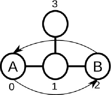
   Create a basic problem that is impossible to solve for the CARP algorithm depicted in Fig. 4(a). Arrows indicate the starting and goal positions of robots $A$ and $B$ on the graph. CARP fails because the agents need to swap their positions while having the same distance to the only node they can use to avoid each other. Because CARP plans agents sequentially one by one while ignoring the subsequent agents, no ordering of these agents can solve this issue.

2. 2.

   Pick random node that has only one edge associated with it.

3. 3.

   Either add 2 nodes $A$ and $B$ to either side of this node if possible along with corresponding assignment of 2 agents – The first agent going from $A$ to $B$ and the second one from $B$ to $A$. The example of this step can be seen in Fig. 4(b). The alternative method to expand the map is to connect the same structure to it as in the Step 1 together with the same type of assignment, the example of which can be seen in Fig. 4(c).

4. 4.

   Repeat Steps 2 and 3 until the map of a required size is generated.

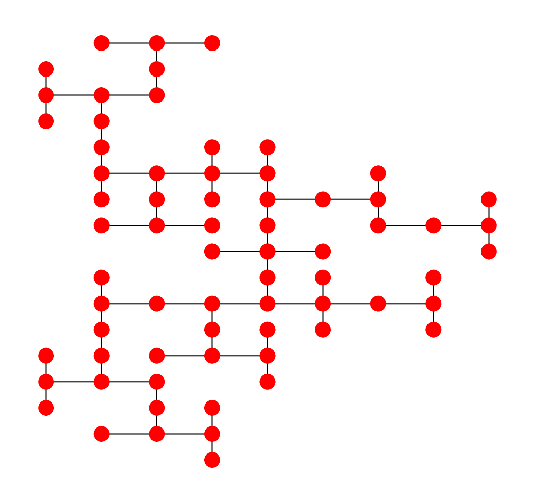
The example of a fully generated map following the previous steps can be seen in Fig. 5.

The second set of experiments was carried out on the second set of maps with the aim to illustrate the behavior of the proposed algorithm on assignments that CARP algorithm can not solve. The total of 400 different combinations of a map and assignment were generated: 100 each for 10, 20, 30 and 40 agents. The results of this experiment can be seen in Fig. 6. The setup numbers 1 to 4 correspond to the number of agents 10 to 40 respectively.

For up to 30 agents the success rate is 100% while it is decreased to 95% for 40 robots. Regarding the computational time results, the algorithm takes approximately 1 second to calculate the paths for each agent in assignments that are impossible to solve for CARP algorithm for up to 30 agents even with relatively complicated assignments.

In this paper, we presented a novel algorithm for coordination of a fleet of robots on a graph. The algorithm is based on a discrete version of RRT for multiple robots (MRdRRT), but it significantly improves particular steps of this algorithm which allows it to solve problems assuming tens of robots in few seconds. This is in contrast to the original MRdRRT which can solve problems up to ten robots in tens of seconds. The experimental comparison moreover shows that the proposed approach can solve problems unsolvable for CARP which is one of the best practical algorithms nowadays. Finally, our approach is comparable to CARP in computational time and quality of the generated solutions for problems with up to 100 robots which are solvable by CARP. The main drawback is that the computational complexity with respect to the number of robots is still exponential.

The ideas of RRT* showed promise in bringing the obtained solution closer to optimum, but for the cost of increased execution time. For this reason, the future work should focus on improvement of the proposed algorithm in terms of reducing the number of required iterations to find the first solution. This could be done for example by reducing the dimensionality of the problem by planning smaller groups of agents in batches and then considering them as obstacles moving in time for the subsequent groups.

REFERENCES

- Bennewitz et al., 2001 Bennewitz, M., Burgard, W., and Thrun, S. (2001). Optimizing schedules for prioritized path planning of multi-robot systems. In Robotics and Automation, 2001. Proceedings 2001 ICRA. IEEE International Conference on, pages 271 – 276 vol.1.
- Cap et al., 2015 Cap, M., Novak, P., Kleiner, A., Selecky, M., and Pechoucek, M. (2015). Prioritized Planning Algorithms for Trajectory Coordination of Multiple Mobile Robots. IEEE Transactions on Automation Science and Engineering, Special Is.
- Chiew, 2010 Chiew, K. (2010). Scheduling and routing of autonomous moving objects on a mesh topology. Operational Research, 12(3):385–397.
- DeWilde et al., 2014 DeWilde, B., Ter Mors, A., and Witteveen, C. (2014). Push and Rotate: A complete Multi-agent Pathfinding algorithm. Journal of Artificial Intelligence Research, 51:443–492.
- Dobson et al., 2017 Dobson, A., Solovey, K., Shome, R., Halperin, D., and Bekris, K. E. (2017). Scalable asymptotically-optimal multi-robot motion planning. In 2017 International Symposium on Multi-Robot and Multi-Agent Systems (MRS), pages 120–127.
- Geramifard et al., 2006 Geramifard, A., Chubak, P., and Bulitko, V. (2006). Biased Cost Pathfinding. In AAAI Conference on Artificial Intelligence and Interactive Digital Entertainment, pages 112–114.
- Goldreich, 2011 Goldreich, O. (2011). Finding the Shortest Move-Sequence in the Graph-Generalized 15-Puzzle Is NP-Hard. In Goldreich, O., editor, Studies in Complexity and Cryptography. Miscellanea on the Interplay between Randomness and Computation - In Collaboration with Lidor Avigad, Mihir Bellare, Zvika Brakerski, Shafi Goldwasser, Shai Halevi, Tali Kaufman, Leonid Levin, Noam Nisan, Dana Ron,, volume 6650 of Lecture Notes in Computer Science, pages 1–5. Springer.
- Hopcroft et al., 1984 Hopcroft, J., Schwartz, J., and Sharir, M. (1984). On the Complexity of Motion Planning for Multiple Independent Objects; PSPACE- Hardness of the ”Warehouseman’s Problem”. The International Journal of Robotics Research, 3(4):76–88.
- Karaman and Frazzoli, 2010 Karaman, S. and Frazzoli, E. (2010). Incremental sampling-based algorithms for optimal motion planning. CoRR, abs/1005.0416.
- Kiril Solovey, 2014 Kiril Solovey, Oren Salzman, D. H. (2014). Finding a needle in an exponential haystack: Discrete rrt for exploration of implicit roadmaps in multi-robot motion planning. Algorithmic Foundations of Robotics XI, pages 591–607.
- Latombe, 1991 Latombe, J.-C. (1991). Robot Motion Planning. Kluwer Academic Publishers, Norwell, MA, USA.
- LaValle and Hutchinson, 1998 LaValle, S. and Hutchinson, S. (1998). Optimal motion planning for multiple robots having independent goals. IEEE Transactions on Robotics and Automation, 14(6):912–925.
- Lavalle, 1998 Lavalle, S. M. (1998). Rapidly-Exploring Random Trees: A New Tool for Path Planning. Technical Report (Computer Science Deptartment, Iowa State University), 11.
- Luna and Bekris, 2011 Luna, R. and Bekris, K. E. (2011). Efficient and complete centralized multi-robot path planning. In 2011 IEEE/RSJ International Conference on Intelligent Robots and Systems, pages 3268–3275. IEEE.
- Parker, 2009 Parker, L. E. (2009). Path Planning and Motion Coordination in Multiple Mobile Robot Teams. Encyclopedia of Complexity and System Science.
- Peasgood et al., 2008 Peasgood, M., Clark, C. M., and McPhee, J. (2008). A Complete and Scalable Strategy for Coordinating Multiple Robots Within Roadmaps. Robotics, IEEE Transactions on, 24(2):283–292.
- Ryan, 2008 Ryan, M. R. (2008). Exploiting Subgraph Structure in Multi-Robot Path Planning. Journal of Artificial Intelligence Research, pages 497–542.
- Silver, 2005 Silver, D. (2005). Cooperative Pathfinding. In The 1st conference on Artificial Intelligence and Interactive Digital Entertainment, pages 117–122.
- Simeon et al., 2002 Simeon, T., Leroy, S., and Lauumond, J.-P. (2002). Path coordination for multiple mobile robots: a resolution-complete algorithm. IEEE Transactions on Robotics and Automation, 18(1):42–49.
- ter Mors et al., 2010 ter Mors, A. W., Witteveen, C., Zutt, J., and Kuipers, F. A. (2010). Context-aware route planning. In Dix, J. and Witteveen, C., editors, Multiagent System Technologies, pages 138–149, Berlin, Heidelberg. Springer Berlin Heidelberg.
- van den Berg and Overmars, 2005 van den Berg, J. and Overmars, M. (2005). Prioritized motion planning for multiple robots. In 2005 IEEE/RSJ International Conference on Intelligent Robots and Systems, pages 430–435. IEEE.
- van den Berg et al., 2009 van den Berg, J., Snoeyink, J., Lin, M. C., and Manocha, D. (2009). Centralized path planning for multiple robots: Optimal decoupling into sequential plans. In Trinkle, J., Matsuoka, Y., and Castellanos, J. A., editors, Robotics: Science and Systems V, University of Washington, Seattle, USA, June 28 - July 1, 2009. The {MIT} Press.
- Wang and Botea, 2008 Wang, K.-H. C. and Botea, A. (2008). Fast and Memory-Efficient Multi-Agent Pathfinding. In ICAPS, pages 380–387.
- Wang and Goh, 2015 Wang, W. and Goh, W. B. (2015). A stochastic algorithm for makespan minimized multi-agent path planning in discrete space. Applied Soft Computing, 30:287–304.