跳到论文正文
W Papers独立论文阅读器 arXiv:1901.07270 论文正文 计算阅读时间 · 0%
引用这篇论文根据当前论文元数据生成,正式投稿前建议核对。


License: arXiv.org perpetual non-exclusive license
arXiv:1901.07270v1 [math.PR] 22 Jan 2019

Constrained Optimal Stopping, Liquidity and Effort

David Hobson Thanks: University of Warwick, Coventry, CV4 7AL, d.hobson@warwick.ac.uk    Matthew Zeng Thanks: University of Warwick, Coventry, CV4 7AL, m.zeng@warwick.ac.uk
August 11, 2026
Abstract

In a classical optimal stopping problem in continuous time, the agent can choose any stopping time without constraint. Dupuis and Wang (Optimal stopping with random intervention times, Advances in Applied Probability, 34, 141–157, 2002) introduced a constraint on the class of admissible stopping times which was that they had to take values in the set of event times of an exogenous, time-homogeneous Poisson process. This can be thought of as a model of finite liquidity. In this article we extend the analysis of Dupuis and Wang to allow the agent to choose the rate of the Poisson process. Choosing a higher rate leads to a higher cost. Even for a simple model for the stopped process and a simple call-style payoff, the problem leads to a rich range of optimal behaviours which depend on the form of the cost function. Often the agent accepts the first offer — if they are not going to accept an offer then there is no point in putting in effort to generate offers, and thus there may be no offers to accept or decline — but for some set-ups this is not the case.

1 Introduction

Optimal stopping problems are widespread in economics and finance (and other fields) where they are used to model asset sales, investment times and the exercise of American-style options. In typical applications an agent observes a stochastic process, possibly representing the price of an asset, and chooses a stopping time in order to maximise the expected discounted value of a payoff which is contingent upon the process evaluated at that time.

Implicit in the classical version of the above problem is the idea that the agent can sell the asset (decide to invest, exercise the option) at any moment of their choosing, and for financial assets traded on an exchange this is a reasonable assumption. However, for other classes of assets, including those described as ‘real assets’ by, for example, Dixit and Pindyck [2], this assumption may be less plausible. Here we are motivated by an interpretation of the optimal stopping problem above in which an agent has an asset for sale, but can only complete the sale if they can find a buyer, and candidate buyers are only available at certain isolated instants of time.

In this work we model the arrival of candidate purchasers as the event times of a Poisson process. When a candidate purchaser arrives the agent can choose to sell to that purchaser, or not; if a sale occurs then the problem terminates, otherwise the candidate purchaser is lost, and the problem continues. If the Poisson process has a constant rate, then the analysis falls into the framework studied by Dupuis and Wang [3] and Lempa [5].

Dupuis and Wang [3] and Lempa [5] discuss optimal stopping problems, but closely related is the work of Rogers and Zane [12] in the context of portfolio optimisation. Rogers and Zane consider an optimal investment portfolio problem under the hypothesis that the portfolio can only be rebalanced at event times of a Poisson process of constant rate, see also Pham and Tankov [10] and Ang, Papanikolaou and Westerfield [1]. The study of optimal stopping problems when the stopping times are constrained to be event times of an exogenous process is relatively unexplored, but Guo and Liu [4] study a problem in which the aim is to maximise a payoff contingent upon the maximum of an exponential Brownian motion and Menaldi and Robin [8] extend the analysis of Dupuis and Wang [3] to consider non-exponential inter-arrival times. As a generalisation of optimal stopping, Liang and Wei [6] consider an optimal switching problem when the switching times are constrained to be event times of a Poisson process.

In this article we consider a more sophisticated model of optimal stopping under constraints in which the agent may expend effort in order to increase the frequency of the arrival times of candidate buyers. (Note that the problem remains an optimal stopping problem, since at each candidate sale opportunity the agent optimises between continuing and selling.) In our model the agent’s instantaneous effort rate EtE_{t} affects the instantaneous rate Λt\Lambda_{t} of the Poisson process, so that the candidate sale opportunities become the event times of an inhomogeneous Poisson process, where the agent chooses the rate. However, this effort is costly, and the agent incurs a cost per unit time which depends on the instantaneous effort rate. The objective of the agent is to maximise the expected discounted payoff net of the expected discounted costs. In particular, if X=(Xt)t≥0X=(X_{t})_{t\geq 0} with X0=xX_{0}=x is the asset price process, gg is the payoff function, β\beta is the discount factor, E=(Et)t≥0E=(E_{t})_{t\geq 0} is the chosen effort process, Λ=(Λt)t≥0\Lambda=(\Lambda_{t})_{t\geq 0} given by Λt=Ψ⁡(Et)\Lambda_{t}=\Psi(E_{t}) is the instantaneous rate of the Poisson process, CEC_{E} is the cost function so that the cost incurred per unit time is CE​(Et)C_{E}(E_{t}), and TΛT_{\Lambda} is the set of event times of a Poisson process, rate Λ\Lambda, then the objective of the agent is to maximise the objective function

𝔼x​[e−β​τ​g​(Xτ)−∫0τe−β​s​CE​(Es)​𝑑s]\mathbb{E}^{x}\left[e^{-\beta\tau}g(X_{\tau})-\int_{0}^{\tau}e^{-\beta s}C_{E}(E_{s})ds\right] (1)

over admissible effort processes EE and TΛT_{\Lambda}-valued stopping times τ\tau. Our goal is to solve for the value function, the optimal stopping time and the optimal effort, as represented by the optimal control process EE. In fact, typically it is possible to use the rate of the Poisson process as the control variable by setting C⁡(Λt)=CE​(Et)=CE∘Ψ−1​(Λt)C(\Lambda_{t})=C_{E}(E_{t})=C_{E}\circ\Psi^{-1}(\Lambda_{t}). In the context of the problem it is natural to assume that Ψ\Psi and CEC_{E} are increasing functions, so that Ψ−1\Psi^{-1} exists, and CC is increasing.

Our focus is on the case where XX is an exponential Brownian motion, but the general case of a regular, time-homogeneous diffusion can be reduced to this case at the expense of slightly more complicated technical conditions. See Lempa [5] for a discussion in the constant arrival rate case. We begin by rigorously stating the form of the problem we will study. Then we proceed to solve for the effort process and stopping rule in (1). It turns out that there are two distinctive cases depending on the shape of CC or more precisely on the finiteness or otherwise of limλ↑∞C⁡(λ)λ\lim_{\lambda\uparrow\infty}\frac{C(\lambda)}{\lambda}. Note that it is not clear a priori what shape C=CE∘Ψ−1C=C_{E}\circ\Psi^{-1} should take, beyond the fact that it is increasing. Generally one might expect an increasing marginal cost of effort and a law of diminishing returns to effort which would correspond to convex CEC_{E}, concave Ψ\Psi and convex CC. But a partial reverse is also conceivable: effort expended below a threshold has little impact, and it is only once effort has reached a critical threshold that extra effort readily yields further stopping opportunities; in this case Ψ\Psi would be convex and CC might be concave.

One outcome of our analysis is that the agent exerts effort to create a positive stopping rate only if they are in the region where stopping is optimal. Outside this region, they typically exert no effort, and there are no stopping opportunities. Typically therefore, (although we give a counterexample in an untypical case) the agent stops at the first occasion where stopping is possible and the optimal stopping element of the problem is trivial.

2 The set-up

We work on a filtered probability space (Ω,ℱ,ℙ,𝔽=(ℱt)t≥0)(\Omega,\mathcal{F},\mathbb{P},\mathbb{F}=(\mathcal{F}_{t})_{t\geq 0}) which satisfies the usual conditions and which supports a Brownian motion and an independent Poisson process. On this space there is a regular, time-homogeneous diffusion process X=(Xt)t≥0X=(X_{t})_{t\geq 0} driven by the Brownian motion. We will assume that XX is exponential Brownian motion with volatility σ\sigma and drift μ\mu and has initial value xx; then

d​Xt=σ​d​Wt+μ​d​t,X0=x.dX_{t}=\sigma dW_{t}+\mu dt,\hskip 28.45274ptX_{0}=x.

Here μ\mu and σ\sigma are constants with μ<β\mu<\beta. The agent has a perpetual option with increaing payoff g:ℝ+↦ℝ+g:\mathbb{R}_{+}\mapsto\mathbb{R}_{+} of linear growth. In our examples gg is an American call: g⁡(x)=(x−K)+g(x)=(x-K)_{+}. Then, in the classical setting, the problem of the agent would be to maximise 𝔼⁡[e−β​τ​g​(Yτ)]\mathbb{E}[e^{-\beta\tau}g(Y_{\tau})] over stopping times τ\tau. Note that the linear growth condition, together with μ<β\mu<\beta, is sufficient to ensure that this classical problem is well-posed.

We want to introduce finite liquidity into this problem, in the sense that we want to incorporate the phenomena that in order to sell the agent needs to find a buyer, and such buyers are in limited supply. In the simplest case buyers might arrive at event times of a time-homogeneous Poisson process with rate λ\lambda, and then at each event time of the Poisson process the agent faces a choice of whether to sell to this buyer at this moment or not; if yes then the sale occurs and the optimal stopping problem terminates, if no then the buyer is irreversibly lost, and the optimal stopping problem continues. We want to augment this problem to allow the agent to expend effort (via networking, research or advertising) in order to increase the flow of buyers. There is a cost of searching in this way — the higher the effort the higher the rate of candidate stopping times but also the higher the search costs. Note that once the asset is sold, effort expended on searching ceases, and search costs thereafter are zero by fiat.

Let 𝒜E\mathcal{A}_{E} be the set of admissible effort processes. We assume that E∈𝒜EE\in\mathcal{A}_{E} if E=(Et)t≥0E=(E_{t})_{t\geq 0} is an adapted process such that Et∈IEE_{t}\in I_{E} for all t∈[0,∞)t\in[0,\infty) where IE⊂ℝ+I_{E}\subset\mathbb{R}_{+} is an interval which is independent of time. Then, since Λt=Ψ⁡(Et)\Lambda_{t}=\Psi(E_{t}) we find E∈𝒜EE\in\mathcal{A}_{E} if and only if Λ∈𝒜\Lambda\in\mathcal{A} where Λ∈𝒜\Lambda\in\mathcal{A} if Λ\Lambda is adapted and Λt∈I\Lambda_{t}\in I for all tt where I=Ψ⁡(IE)I=\Psi(I_{E}). Note that II is an interval in ℝ+\mathbb{R}_{+}, and we take the lower and upper endpoints to be λ¯\underline{\lambda} and λ¯\overline{\lambda} respectively.

Recall that TΛT_{\Lambda} is the set of event times of an inhomogeneous Poisson process with rate Λ\Lambda. Then TΛ={T1Λ,T2Λ,…}T^{\Lambda}=\{T^{\Lambda}_{1},T^{\Lambda}_{2},\ldots\} where 0<T1Λ0<T^{\Lambda}_{1} and TnΛ<Tn+1ΛT^{\Lambda}_{n}<T^{\Lambda}_{n+1} almost surely. Let 𝒯⁡(TΛ)\mathcal{T}(T_{\Lambda}) be the set of TΛT_{\Lambda}-valued stopping times and let 𝒜\mathcal{A} be the set of admissible rate functions. Then, after a change of independent variable the problem is to find

H⁡(x)=supΛ∈𝒜supτ∈𝒯⁡(TΛ)𝔼x​[e−β​τ​g​(Xτ)−∫0τe−β​s​C​(Λs)​𝑑s],H(x)=\sup_{\Lambda\in\mathcal{A}}\sup_{\tau\in\mathcal{T}(T_{\Lambda})}\mathbb{E}^{x}\left[e^{-\beta\tau}g(X_{\tau})-\int_{0}^{\tau}e^{-\beta s}C(\Lambda_{s})ds\right], (2)

together with the optimal rate function Λ∗=(Λt∗)t≥0\Lambda^{*}=(\Lambda^{*}_{t})_{t\geq 0} and optimal stopping rule τ∗∈𝒯⁡(TΛ)\tau^{*}\in\mathcal{T}(T_{\Lambda}).

In addition to the set of admissible controls, we also consider the subset of integrable controls ℐ⊆𝒜\mathcal{I}\subseteq\mathcal{A} where Λ∈ℐ=ℐ⁡(I,C)\Lambda\in\mathcal{I}=\mathcal{I}(I,C) is an adapted process with Λt∈I\Lambda_{t}\in I for which 𝔼x​[∫0∞e−β​s​C​(Λs)​𝑑s]<∞\mathbb{E}^{x}[\int_{0}^{\infty}e^{-\beta s}C(\Lambda_{s})ds]<\infty. As mentioned above we have that 𝔼x​[e−β​τ​g​(Xτ)]<∞\mathbb{E}^{x}\left[e^{-\beta\tau}g(X_{\tau})\right]<\infty for any admissible Λ\Lambda and any stopping rule, and hence there is no loss of generality in restricting the search for the optimal rate function to the set of integrable controls.

The stopping rule is easily identified in feedback form. Let TΛ0=TΛ∪{0}T^{0}_{\Lambda}=T_{\Lambda}\cup\{0\} and let H0H^{0} be the value of the problem conditional on there being a buyer available at time 0, so that

H0​(x)=supΛ∈𝒜supτ∈𝒯⁡(TΛ0)𝔼x​[e−β​τ​g​(Xτ)−∫0τe−β​s​C​(Λs)​𝑑s].H^{0}(x)=\sup_{\Lambda\in\mathcal{A}}\sup_{\tau\in\mathcal{T}(T^{0}_{\Lambda})}\mathbb{E}^{x}\left[e^{-\beta\tau}g(X_{\tau})-\int_{0}^{\tau}e^{-\beta s}C(\Lambda_{s})ds\right].

Then, it is optimal to stop immediately if and only if the value of stopping is at least as large as the value of continuing and

H0​(x)=max⁡{g⁡(x),H⁡(x)}.H^{0}(x)=\max\{g(x),H(x)\}.

It follows that if Λ=(Λt)t≥0\Lambda=(\Lambda_{t})_{t\geq 0} is a fixed admissible rate process, and if HΛ0H^{0}_{\Lambda} and HΛH_{\Lambda} denote the respective value functions then, writing T1=T1ΛT_{1}=T^{\Lambda}_{1} for the first event time of the Poisson process with rate Λ\Lambda,

HΛ​(x)\displaystyle H_{\Lambda}(x) =\displaystyle= supτ∈𝒯⁡(TΛ)𝔼x​[e−β​τ​g​(Xτ)−∫0τe−β​s​C​(Λs)​𝑑s]\displaystyle\sup_{\tau\in\mathcal{T}(T_{\Lambda})}\mathbb{E}^{x}\left[e^{-\beta\tau}g(X_{\tau})-\int_{0}^{\tau}e^{-\beta s}C(\Lambda_{s})ds\right]
=\displaystyle= supτ∈𝒯⁡(TΛ)𝔼x[e−β​T1𝔼[e−β⁡(τ−T1)g(Xτ)−∫T1τe−β⁡(s−T1)C(Λs)ds|ℱT1]−∫0T1e−β​sC(Λs)ds]\displaystyle\sup_{\tau\in\mathcal{T}(T_{\Lambda})}\mathbb{E}^{x}\left[e^{-\beta T_{1}}\mathbb{E}\left[\left.e^{-\beta(\tau-T_{1})}g(X_{\tau})-\int_{T_{1}}^{\tau}e^{-\beta(s-T_{1})}C(\Lambda s)ds\right|\mathcal{F}_{T_{1}}\right]-\int_{0}^{T_{1}}e^{-\beta s}C(\Lambda_{s})ds\right]
=\displaystyle= 𝔼x[e−β​T1HΛ0(XT1)−∫0∞I{s<T1}e−β​sC(Λs)ds]\displaystyle\mathbb{E}^{x}\left[e^{-\beta T_{1}}H^{0}_{\Lambda}(X_{T_{1}})-\int_{0}^{\infty}I_{\{s<T_{1}\}}e^{-\beta s}C(\Lambda_{s})ds\right]
=\displaystyle= 𝔼x[∫0∞Λse−∫0sΛudue−β​sHΛ0(Xs)ds−∫0∞e−∫0sΛudue−β​sC(Λs)ds]\displaystyle\mathbb{E}^{x}\left[\int_{0}^{\infty}\Lambda_{s}e^{-\int_{0}^{s}\Lambda_{u}du}e^{-\beta s}H^{0}_{\Lambda}(X_{s})ds-\int_{0}^{\infty}e^{-\int_{0}^{s}\Lambda_{u}du}e^{-\beta s}C(\Lambda_{s})ds\right]
=\displaystyle= 𝔼x​[∫0∞e−(β​s+∫0sΛu​𝑑u)​(Λs​HΛ0​(Xs)​𝑑s−C⁡(Λs))​𝑑s].\displaystyle\mathbb{E}^{x}\left[\int_{0}^{\infty}e^{-(\beta s+\int_{0}^{s}\Lambda_{u}du)}(\Lambda_{s}H^{0}_{\Lambda}(X_{s})ds-C(\Lambda_{s}))ds\right].

Taking a supremum over admissible rate processes Λ∈𝒜\Lambda\in\mathcal{A} we find

H(x)=supΛ∈𝒜𝔼x[∫0∞e−∫0t(β+Λs)ds(ΛtHΛ0(Xt)−C(Λt))dt],H(x)=\sup_{\Lambda\in\mathcal{A}}\mathbb{E}^{x}\left[\int_{0}^{\infty}e^{-\int_{0}^{t}(\beta+\Lambda_{s})ds}\left(\Lambda_{t}H_{\Lambda}^{0}(X_{t})-C(\Lambda_{t})\right)dt\right],

and this is the problem we aim to solve. Writing Λ∗\Lambda^{*} for the optimal rate process we expect HH to solve

H(x)=𝔼x[∫0∞e−∫0t(β+Λ∗s)ds(Λt∗{g(Xt)∨H(Xt)}−C(Λt∗))dt].H(x)=\mathbb{E}^{x}\left[\int_{0}^{\infty}e^{-\int_{0}^{t}(\beta+\Lambda^{*}_{s})ds}\left(\Lambda^{*}_{t}\{g(X_{t})\vee H(X_{t})\}-C(\Lambda^{*}_{t})\right)dt\right].

2.1 Some results for classical problems

For future reference we record some results for classical problems in which agents can stop at any instant.

First, let 𝒯⁡([0,∞))\mathcal{T}([0,\infty)) be the set of all stopping times and define

wK​(x):=supτ∈𝒯⁡([0,∞))𝔼x​[e−β​τ​(Xτ−K)+].w_{K}(x):=\sup_{\tau\in\mathcal{T}([0,\infty))}\mathbb{E}^{x}[e^{-\beta\tau}(X_{\tau}-K)_{+}].

(Imagine a standard, perpetual, American-style call option with strike KK, though valuation is not taking place under the equivalent martingale measure.) Classical arguments (McKean [7], Peskir and Shiryaev [9]) give that 0<wK<x0<w_{K}<x (the upper bound holds since we are assuming β>μ\beta>\mu) and that there exists a constant L=θθ−1​KL=\frac{\theta}{\theta-1}K where θ=(12−μσ2)+(12−μσ2)2+2​βσ2\theta=\left(\frac{1}{2}-\frac{\mu}{\sigma^{2}}\right)+\sqrt{\left(\frac{1}{2}-\frac{\mu}{\sigma^{2}}\right)^{2}+\frac{2\beta}{\sigma^{2}}} such that

wK​(x)={(x−K)+,x>L;(L−K)​L−θ​xθ,0<x≤L.w_{K}(x)=\left\{\begin{array}[]{ll}(x-K)_{+},&x>L;\\ (L-K)L^{-\theta}x^{\theta},&0<x\leq L.\end{array}\right.

For future reference set ϕ=(12−μσ2)−(12−μσ2)2+2​βσ2\phi=\left(\frac{1}{2}-\frac{\mu}{\sigma^{2}}\right)-\sqrt{\left(\frac{1}{2}-\frac{\mu}{\sigma^{2}}\right)^{2}+\frac{2\beta}{\sigma^{2}}}. Then ϕ<0<1<θ\phi<0<1<\theta and θ\theta and ϕ\phi are the roots of Q0=0Q_{0}=0 where Qλ​(ψ)=12​σ2​ψ​(ψ−1)+μ​ψ−(β+λ)Q_{\lambda}(\psi)=\frac{1}{2}\sigma^{2}\psi(\psi-1)+\mu\psi-(\beta+\lambda).

Second, define

wK,ϵ,δ​(x)=supτ∈𝒯⁡([0,∞))𝔼x​[e−β​τ​{(Xτ−K)+−ϵ}−δ​∫0τe−β​s​𝑑s].w_{K,\epsilon,\delta}(x)=\sup_{\tau\in\mathcal{T}([0,\infty))}\mathbb{E}^{x}\left[e^{-\beta\tau}\{(X_{\tau}-K)_{+}-\epsilon\}-\delta\int_{0}^{\tau}e^{-\beta s}ds\right]. (3)

(Imagine a perpetual, American-style call option with strike KK, in which the agent pays a fee or transaction cost ϵ\epsilon to exercise the option, and pays a running cost δ\delta per unit time until the option is exercised.) Note that wK,0,0≡wKw_{K,0,0}\equiv w_{K}. It turns out that there are two cases. In the first case when ϵ≥δ/β\epsilon\geq\delta/\beta, when XX is small it is more cost effective to pay the running cost indefinitely than to pay the exercise fee. We find

wK,ϵ,δ​(x)=wK+ϵ−δ/β​(x)−δ/β.w_{K,\epsilon,\delta}(x)=w^{K+\epsilon-\delta/\beta}(x)-\delta/\beta.

In the second case when ϵ<δ/β\epsilon<\delta/\beta, when XX is small it is cost-effective to stop immediately, even though the payoff is zero, because paying the fee is cheaper than paying the running cost indefinitely. In this case we find that w=wK,ϵ,δw=w_{K,\epsilon,\delta} and a pair of thresholds l∗=l∗​(K,ϵ,δ)l^{*}=l^{*}(K,\epsilon,\delta) and L∗=L∗​(K,ϵ,δ)L^{*}=L^{*}(K,\epsilon,\delta) with 0<l∗<K+ϵ<L∗0<l^{*}<K+\epsilon<L^{*} satisfy the variational problem

{w is C1; w=−ϵ on (0,l∗); ℒ​w−β​w=δ on (l∗,L∗); w=x−K−ϵ on (L∗,∞) }\{\mbox{$w$ is $C^{1}$; $w=-\epsilon$ on $(0,l^{*})$; $\mathcal{L}w-\beta w=\delta$ on $(l^{*},L^{*})$; $w=x-K-\epsilon$ on $(L^{*},\infty)$ }\}

Returning to our problem with limited stopping opportunities, one immediate observation is that H​(x)≤wK​(x)H(x)\leq w_{K}(x). Conversely, if Λ≡0\Lambda\equiv 0 is admissible then H⁡(x)≥−C⁡(0)βH(x)\geq-\frac{C(0)}{\beta}.

3 Heuristics

From the Markovian structure of the problem we expect that the (unknown) value function HH and optimal rate function Λ∗\Lambda^{*} are time-homogeneous functions of the asset price only.

Let MΛ=(MtΛ)t≥0M^{\Lambda}=(M^{\Lambda}_{t})_{t\geq 0} be given by

MtΛ=e−∫0t(β+Λs)dsH(Xt)+∫0te−∫0u(β+Λs)ds[ΛuH0(Xu)−C(Λu)]du,M^{\Lambda}_{t}=e^{-\int_{0}^{t}(\beta+\Lambda_{s})ds}H(X_{t})+\int_{0}^{t}e^{-\int_{0}^{u}(\beta+\Lambda_{s})ds}\left[\Lambda_{u}H^{0}(X_{u})-C(\Lambda_{u})\right]du,

and let ℒX\mathcal{L}^{X} denote the generator of XX so that ℒX​f=σ22​f′′+μ​f′\mathcal{L}^{X}f=\frac{\sigma^{2}}{2}f^{\prime\prime}+\mu f^{\prime}. Assume that the value function under the optimal strategy HH is C2C^{2}. Then, by Itô’s formula,

dMtΛ=e−∫0t(β+Λs)ds{(ℒXH(Xt)−(β+Λt)H(Xt)+Λt(H0(Xt)−C(Λt)))dt+σXtH′(Xt)dWt}.dM^{\Lambda}_{t}=e^{-\int_{0}^{t}(\beta+\Lambda_{s})ds}\left\{\left(\mathcal{L}^{X}H(X_{t})-(\beta+\Lambda_{t})H(X_{t})+\Lambda_{t}(H^{0}(X_{t})-C(\Lambda_{t}))\right)dt+\sigma X_{t}H^{\prime}(X_{t})dW_{t}\right\}.

We expect that MΛM^{\Lambda} is a super-martingale for any choice of Λ\Lambda, and a martingale for the optimal choice. Thus we expect

ℒX​H​(Xt)−β​H​(Xt)−infΛt{C⁡(Λt)−Λt​[H0​(Xt)−H⁡(Xt)]}=0.\mathcal{L}^{X}H(X_{t})-\beta H(X_{t})-\inf_{\Lambda_{t}}\left\{C(\Lambda_{t})-\Lambda_{t}[H^{0}(X_{t})-H(X_{t})]\right\}=0.

Let C~:ℝ+↦ℝ\tilde{C}:\mathbb{R}_{+}\mapsto\mathbb{R} be the concave conjugate of CC so that C~​(z)=infλ≥0{C⁡(λ)−λ​z}\tilde{C}(z)=\inf_{\lambda\geq 0}\{C(\lambda)-\lambda z\}. Then we find that HH solves

ℒX​H−β​H−C~​(H0−H)=0,\mathcal{L}^{X}H-\beta H-\tilde{C}(H^{0}-H)=0, (4)

and a best choice of rate function is Λt∗=Λ∗​(Xt)\Lambda^{*}_{t}=\Lambda^{*}(X_{t}) where

Λ∗​(x)=Θ⁡(H0​(x)−H⁡(x))\Lambda^{*}(x)=\Theta(H^{0}(x)-H(x)) (5)

and Θ⁡(z)=arginfλ​{C⁡(λ)−λ​z}\Theta(z)=\mbox{arginf}_{\lambda}\{C(\lambda)-\lambda z\}. Note that H0−H=(g−H)+H^{0}-H=(g-H)_{+} and that (4) is a second order differential equation and will have multiple solutions. The boundary behaviour near zero and infinity will determine which solution fits the optimal stopping problem.

3.1 First Example: Quadratic cost functions

Suppose g⁡(x)=(x−K)+g(x)=(x-K)_{+} for fixed K>0K>0. Using terminology from the study of American options and optimal stopping we say that if Xt>KX_{t}>K then the process is in-the-money, if Xt<KX_{t}<K then the process is out-of-the-money and the region in the domain of XX where Λ∗​(X)\Lambda^{*}(X) is zero is the continuation region 𝒞\mathcal{C}, and 𝒮:=ℝ+∖𝒞\mathcal{S}:=\mathbb{R}^{+}\setminus\mathcal{C} is the selling region.

Suppose the range of possible values for the rate process is I=[0,∞)I=[0,\infty) and consider a quadratic cost function C⁡(λ)=a+b​λ+c​λ22C(\lambda)=a+b\lambda+c\frac{\lambda^{2}}{2} with a≥0a\geq 0, b≥0b\geq 0 and c>0c>0. Then C~​(z)=a−[(z−b)+]22​c\tilde{C}(z)=a-\frac{[(z-b)_{+}]^{2}}{2c}.

Consider first the behaviour of the value function near zero. If a=0a=0 then C⁡(0)=0C(0)=0, and when XX is close to zero the agent may choose not to search for buyers, a strategy which incurs zero cost. There is little chance of the process ever being in-the-money, but nonethelesss the agent delays sale indefinitely. We expect that the continuation region is (0,L∗)(0,L^{*}) for some threshold L∗L^{*}.

Now suppose a>0a>0. Now there is a cost to delaying the sale, even when Λ=0\Lambda=0. If XX is small then it is preferable to sell the asset even though the process is out-of-the-money, because in our problem there are no search costs once the asset is sold. In this case we expect the agent to search for buyers when XX is small, in order to reduce further costs. Then the continuation region will be (ℓ∗,L∗)(\ell^{*},L^{*}) for some 0<ℓ∗<K<L∗<∞0<\ell^{*}<K<L^{*}<\infty.

Consider now the behaviour for large xx. In this case we can look for an expansion for the solution of (4) of the form

H(x)=A1x+A1/2x+A0+O(x−1/2)H(x)=A_{1}x+A_{1/2}\sqrt{x}+A_{0}+O(x^{-1/2})

for constants A1A_{1}, A1/2A_{1/2} and A0A_{0} to be determined. Using the fact that H​(x)≤wK​(x)H(x)\leq w_{K}(x) so that HH is of at most linear growth we find

H⁡(x)=x−2​c​(β−μ)​x−{K+b−c⁡[β−μ2+σ28]}+…H(x)=x-\sqrt{2c(\beta-\mu)}\sqrt{x}-\left\{K+b-c\left[\beta-\frac{\mu}{2}+\frac{\sigma^{2}}{8}\right]\right\}+\ldots (6)

Numerical results (see Figure 1) show that this expansion is very accurate for large xx.

3.1.1 Purely quadratic cost: a=0=ba=0=b

In this case we expect that the continuation region is (0,L∗)(0,L^{*}) for a threshold level L∗L^{*} to be determined. For a general threshold LL, and writing HLH_{L} for the solution to (4) with H⁡(0)=0H(0)=0 and H⁡(L)=L−KH(L)=L-K we find that HLH_{L} solves

ℒX​h−β​h=12​c​({g−h}+)2,\mathcal{L}^{X}h-\beta h=\frac{1}{2c}(\{g-h\}_{+})^{2}, (7)

and then that HL​(x)=L−KLθ​xθH_{L}(x)=\frac{L-K}{L^{\theta}}x^{\theta} on x≤Lx\leq L. On (L,∞)(L,\infty), HLH_{L} solves (7) subject to HL​(L)=(L−K)H_{L}(L)=(L-K) and HL′​(L)=θ​L−KLH_{L}^{\prime}(L)=\theta\frac{L-K}{L}. This procedure gives us a family (HL)L≥K(H_{L})_{L\geq K} of potential value functions, each of which is C1C^{1}. Finally we can determine the threshold level LL we need by choosing the value L∗L^{*} for which HL∗H_{L^{*}} has linear growth at infinity.

Refer to caption
(a) For large x
Refer to caption
(b) For small x
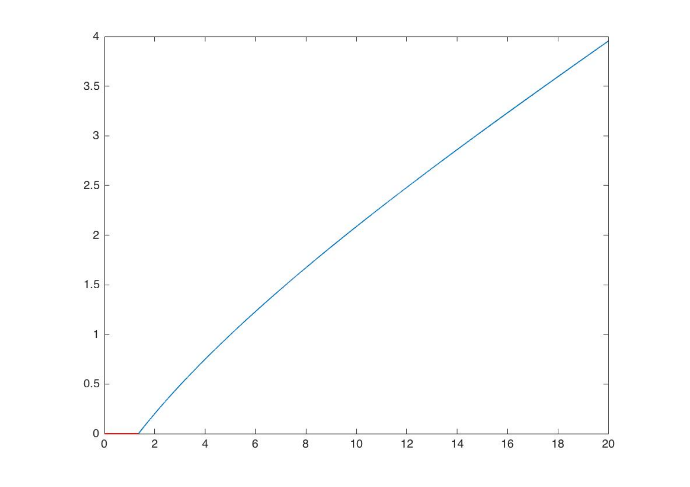
Figure 1: (β,μ,σ,K,a,b,c)=(5,3,2,1,0,0,2)(\beta,\mu,\sigma,K,a,b,c)=(5,3,2,1,0,0,2). In both sub-figures the solid curved line represents HL∗H_{L^{*}}; the straight line represents g∨HL∗g\vee H_{L^{*}} on {x:g⁡(x)≥HL∗​(x)}\{x:g(x)\geq H_{L^{*}}(x)\} and the dashed line in the left sub-figure is the expansion for HH in (6). The optimal threshold is seen in the right sub-figure to be at L∗=1.35L^{*}=1.35.

The linear growth solution HL∗H_{L^{*}} is shown in Figure 1, both for large xx and for moderate xx. From Figure 1(b) we see that the continuation region is 𝒞=(0,1.35)\mathcal{C}=(0,1.35) and that the stopping region 𝒮=[1.35,∞)\mathcal{S}=[1.35,\infty). We also see that the expansion for HH given in (6) gives a good approximation of our numerical solution for large xx.

Refer to caption
Figure 2: (β,μ,σ,K,a,b,c)=(5,3,2,1,0,0,2)(\beta,\mu,\sigma,K,a,b,c)=(5,3,2,1,0,0,2); this figure plots the optimal control Λ∗\Lambda^{*} given by (5) as a function of wealth level xx.

Figure 2 shows the optimal control. We see that Λ∗\Lambda^{*} is zero on the continuation region 𝒞=(0,L)\mathcal{C}=(0,L) and that Λ∗\Lambda^{*} is increasing and concave on the stopping region 𝒮=[L,∞)\mathcal{S}=[L,\infty). The agent behaves rationally in the sense that on the continuation region where continuing is worth more than stopping, the agent is unwilling to stop and this is reflected by the minimal efforts spent on searching (i.e. Λ∗​(x)=0,∀x∈𝒞\Lambda^{*}(x)=0,\forall x\in\mathcal{C}); similarly, on the stopping region, stopping is getting more and more valuable relative to continuing as the price process gets deeper in-the-money, and the agent is incentivised to spend more effort on searching for stopping opportunities.

We discuss the cases of a>0a>0 and b>0b>0 in Section 6.

4 Verification

In this section we show that the heuristics are correct, and that the value to the stochastic problem is given by the appropriate solution of the differential equation. Although the details are different, the structure of the proof follows Dupuis and Wang [3].

Suppose, as throughout, that XX is exponential Brownian motion with μ<β\mu<\beta and gg is of linear growth.

Definition 1.

(τ,Λ)(\tau,\Lambda) is admissible if Λ\Lambda is a non-negative, II-valued, adapted process and τ∈𝒯⁡(TΛ)\tau\in\mathcal{T}(T^{\Lambda}).

Note that a consequence of the definition is that we insist that τ≤T∞Λ:=limnTnΛ\tau\leq T^{\Lambda}_{\infty}:=\lim_{n}T^{\Lambda}_{n}. Moreover, we may have Tk=∞T_{k}=\infty: in this case we may take τ=∞\tau=\infty, whence we have e−β​τ​g​(Xτ)=0e^{-\beta\tau}g(X_{\tau})=0 noting that limt↑∞e−β​t​g​(Xt)=0\lim_{t\uparrow\infty}e^{-\beta t}g(X_{t})=0 almost surely.

Definition 2.

(τ,Λ)(\tau,\Lambda) is integrable if (τ,Λ)(\tau,\Lambda) is admissible and 𝔼⁡[∫0τe−β​s​C​(Λs)​𝑑s]<∞\mathbb{E}[\int_{0}^{\tau}e^{-\beta s}C(\Lambda_{s})ds]<\infty.

Clearly, if (τ,Λ)(\tau,\Lambda) is integrable, then (T1Λ,Λ)(T^{\Lambda}_{1},\Lambda) is integrable.

Lemma 1.

Let GG be an increasing, convex solution to

ℒX​G−β​G−C~​((g−G)+)=0,\mathcal{L}^{X}G-\beta G-\tilde{C}((g-G)_{+})=0, (8)

and suppose that GG is of at most linear growth. Set G0=G∨gG^{0}=G\vee g.

Then for any integrable, admissible strategy (τ,Λ)(\tau,\Lambda),

G(x)≥𝔼x[e−β​T1ΛG0(XT1Λ)I{TΛ1<∞}−∫0T1Λe−β​sC(Λs)ds].G(x)\geq\mathbb{E}^{x}\left[e^{-\beta T^{\Lambda}_{1}}G^{0}(X_{T^{\Lambda}_{1}})I_{\{T^{\Lambda}_{1}<\infty\}}-\int_{0}^{T^{\Lambda}_{1}}e^{-\beta s}C(\Lambda_{s})ds\right]. (9)
Proof.

Since gg and GG are of linear growth we may assume G0​(x)≤κ0+κ1​xG^{0}(x)\leq\kappa_{0}+\kappa_{1}x for some constants κi∈(0,∞)\kappa_{i}\in(0,\infty).

Let Zt=e−β​t−∫0tΛs​𝑑s​G​(Xt)−∫0te−β​s−∫0sΛu​𝑑u​Fs​𝑑sZ_{t}=e^{-\beta t-\int_{0}^{t}\Lambda_{s}ds}G(X_{t})-\int_{0}^{t}e^{-\beta s-\int_{0}^{s}\Lambda_{u}du}F_{s}ds where

Fs=F⁡(g⁡(Xs),G⁡(Xs),Λs):=(g⁡(Xs)−G⁡(Xs))+​Λs+C~​((g⁡(Xs)−G⁡(Xs))+)≤C⁡(Λs).F_{s}=F(g(X_{s}),G(X_{s}),\Lambda_{s}):=(g(X_{s})-G(X_{s}))_{+}\Lambda_{s}+\tilde{C}((g(X_{s})-G(X_{s}))_{+})\leq C(\Lambda_{s}).

Then, using the definition of GG

d​Zt\displaystyle dZ_{t} =\displaystyle= e−β​t−∫0tΛs​𝑑s​{−(β+Λt)​G+ℒX​G−(g−G)+​Λt−C~​((g−G)+)}​d​t+d​Nt\displaystyle e^{-\beta t-\int_{0}^{t}\Lambda_{s}ds}\left\{-(\beta+\Lambda_{t})G+\mathcal{L}^{X}G-(g-G)_{+}\Lambda_{t}-\tilde{C}((g-G)_{+})\right\}dt+dN_{t}
=\displaystyle= e−β​t−∫0tΛs​𝑑s​{−Λt​[G+(g−G)+]}​d​t+d​Nt\displaystyle e^{-\beta t-\int_{0}^{t}\Lambda_{s}ds}\left\{-\Lambda_{t}[G+(g-G)_{+}]\right\}dt+dN_{t}
=\displaystyle= −e−β​t−∫0tΛs​𝑑s​Λt​G0​(Xt)​d​t+d​Nt\displaystyle-e^{-\beta t-\int_{0}^{t}\Lambda_{s}ds}\Lambda_{t}G^{0}(X_{t})dt+dN_{t}

where Nt=∫0te−β​s−∫0sΛu​𝑑u​σ​Xs​G′​(Xs)​d​WsN_{t}=\int_{0}^{t}e^{-\beta s-\int_{0}^{s}\Lambda_{u}du}\sigma X_{s}G^{\prime}(X_{s})dW_{s}. Our hypotheses on GG allow us to conclude that N=(Nt)t≥0N=(N_{t})_{t\geq 0} is a martingale.

It follows that Z0=𝔼⁡[Zt+∫0te−β​s−∫0sΛu​𝑑u​Λs​G0​(Xs)​𝑑s]Z_{0}=\mathbb{E}[Z_{t}+\int_{0}^{t}e^{-\beta s-\int_{0}^{s}\Lambda_{u}du}\Lambda_{s}G^{0}(X_{s})ds] or equivalently

G⁡(x)\displaystyle G(x) =\displaystyle= 𝔼x​[e−β​t−∫0tΛs​𝑑s​G​(Xt)+∫0te−β​s−∫0sΛu​𝑑u​(Λs​(g⁡(Xs)∨G⁡(Xs))−Fs)​𝑑s]\displaystyle\mathbb{E}^{x}\left[e^{-\beta t-\int_{0}^{t}\Lambda_{s}ds}G(X_{t})+\int_{0}^{t}e^{-\beta s-\int_{0}^{s}\Lambda_{u}du}\left(\Lambda_{s}(g(X_{s})\vee G(X_{s}))-F_{s}\right)ds\right] (10)
≥\displaystyle\geq 𝔼x​[e−β​t−∫0tΛs​𝑑s​G​(Xt)+∫0te−β​s−∫0sΛu​𝑑u​(Λs​G0​(Xs)−C⁡(Λs))​𝑑s].\displaystyle\mathbb{E}^{x}\left[e^{-\beta t-\int_{0}^{t}\Lambda_{s}ds}G(X_{t})+\int_{0}^{t}e^{-\beta s-\int_{0}^{s}\Lambda_{u}du}\left(\Lambda_{s}G^{0}(X_{s})-C(\Lambda_{s})\right)ds\right].

Since XX is geometric Brownian motion and β>μ\beta>\mu we have that Xβ,∗:=supu≥0{e−β​u​Xu}X^{\beta,*}:=\sup_{u\geq 0}\{e^{-\beta u}X_{u}\} is in L1L^{1}. Then

e−β​t−∫0tΛs​𝑑s​G​(Xt)\displaystyle e^{-\beta t-\int_{0}^{t}\Lambda_{s}ds}G(X_{t}) ≤\displaystyle\leq κ0+κ1​Xβ,∗,\displaystyle\kappa_{0}+\kappa_{1}X^{\beta,*},
∫0te−β​s−∫0sΛu​𝑑u​Λs​G0​(Xs)​𝑑s\displaystyle\int_{0}^{t}e^{-\beta s-\int_{0}^{s}\Lambda_{u}du}\Lambda_{s}G^{0}(X_{s})ds ≤\displaystyle\leq (κ0+κ1Xβ,∗)∫0tΛse−∫0sΛududs≤κ0+κ1Xβ,∗,\displaystyle(\kappa_{0}+\kappa_{1}X^{\beta,*})\int_{0}^{t}\Lambda_{s}e^{-\int_{0}^{s}\Lambda_{u}du}ds\leq\kappa_{0}+\kappa_{1}X^{\beta,*},
∫0te−β​s−∫0sΛu​𝑑u​C​(Λs)​𝑑s\displaystyle\int_{0}^{t}e^{-\beta s-\int_{0}^{s}\Lambda_{u}du}C(\Lambda_{s})ds ≤\displaystyle\leq ∫0∞e−β​s−∫0sΛu​𝑑u​C​(Λs)​𝑑s,\displaystyle\int_{0}^{\infty}e^{-\beta s-\int_{0}^{s}\Lambda_{u}du}C(\Lambda_{s})ds,

and, since (T1Λ,Λ)(T^{\Lambda}_{1},\Lambda) is integrable by hypothesis,

𝔼⁡[∫0∞e−β​s−∫0sΛu​𝑑u​C​(Λs)​𝑑s]=𝔼⁡[∫0T1Λe−β​s​C​(Λs)​𝑑s]<∞.\mathbb{E}\left[\int_{0}^{\infty}e^{-\beta s-\int_{0}^{s}\Lambda_{u}du}C(\Lambda_{s})ds\right]=\mathbb{E}\left[\int_{0}^{T^{\Lambda}_{1}}e^{-\beta s}C(\Lambda_{s})ds\right]<\infty.

Then Dominated Convergence, together with the fact that e−β​t​Xt→0e^{-\beta t}X_{t}\rightarrow 0 gives (9).

∎

Lemma 2.

Let (τ,Λ)(\tau,\Lambda) be an integrable strategy. Define Y=(Yn)n≥0Y=(Y_{n})_{n\geq 0} by

Yn=e−β⁡(TnΛ∧τ)G0(XTnΛ∧τ)I{TΛn∧τ<∞}−∫0TnΛ∧τe−β​sC(Λs)dsY_{n}=e^{-\beta(T^{\Lambda}_{n}\wedge\tau)}G^{0}(X_{T^{\Lambda}_{n}\wedge\tau})I_{\{T^{\Lambda}_{n}\wedge\tau<\infty\}}-\int_{0}^{T^{\Lambda}_{n}\wedge\tau}e^{-\beta s}C(\Lambda_{s})ds

where T0Λ=0T^{\Lambda}_{0}=0. Define 𝒢n=ℱTnΛ\mathcal{G}_{n}=\mathcal{F}_{T^{\Lambda}_{n}} and set 𝔾=(𝒢n)n≥0\mathbb{G}=(\mathcal{G}_{n})_{n\geq 0}.

Then YY is a uniformly integrable (𝒢n)n≥0(\mathcal{G}_{n})_{n\geq 0}-supermartingale.

Proof.

We have

|Yn|≤κ0+κ1​Xβ,∗+∫0τe−β​s​C​(Λs)​𝑑s∈L1.|Y_{n}|\leq\kappa_{0}+\kappa_{1}X^{\beta,*}+\int_{0}^{\tau}e^{-\beta s}C(\Lambda_{s})ds\in L^{1}.

Moreover, on Tn−1Λ<∞T^{\Lambda}_{n-1}<\infty and τ>Tn−1Λ\tau>T^{\Lambda}_{n-1}, writing T~\tilde{T} as shorthand for TnΛ−Tn−1ΛT^{\Lambda}_{n}-T^{\Lambda}_{n-1} and using τ≥TnΛ\tau\geq T^{\Lambda}_{n} and Lemma 1 for the crucial first inequality,

𝔼⁡[Yn|𝒢n−1]\displaystyle\mathbb{E}[Y_{n}|\mathcal{G}_{n-1}] =\displaystyle= e−β​Tn−1Λ𝔼[e−β​T~G0(XTnΛ)I{TΛn<∞}−∫Tn−1ΛTnΛe−β​sC(Λs)ds|𝒢n−1]−∫0Tn−1Λe−β​sC(Λs)ds\displaystyle e^{-\beta T^{\Lambda}_{n-1}}\mathbb{E}\left[\left.e^{-\beta\tilde{T}}G^{0}(X_{T^{\Lambda}_{n}})I_{\{T^{\Lambda}_{n}<\infty\}}-\int_{T^{\Lambda}_{n-1}}^{T^{\Lambda}_{n}}e^{-\beta s}C(\Lambda_{s})ds\right|\mathcal{G}_{n-1}\right]-\int_{0}^{T^{\Lambda}_{n-1}}e^{-\beta s}C(\Lambda_{s})ds
≤\displaystyle\leq e−β​Tn−1Λ​G​(XTn−1Λ)−∫0Tn−1Λe−β​s​C​(Λs)​𝑑s\displaystyle e^{-\beta T^{\Lambda}_{n-1}}G(X_{T^{\Lambda}_{n-1}})-\int_{0}^{T^{\Lambda}_{n-1}}e^{-\beta s}C(\Lambda_{s})ds
≤\displaystyle\leq e−β​Tn−1Λ​G0​(XTn−1Λ)−∫0Tn−1Λe−β​s​C​(Λs)​𝑑s=Yn−1.\displaystyle e^{-\beta T^{\Lambda}_{n-1}}G^{0}(X_{T^{\Lambda}_{n-1}})-\int_{0}^{T^{\Lambda}_{n-1}}e^{-\beta s}C(\Lambda_{s})ds=Y_{n-1}.

∎

Proposition 1.

Let GG be an increasing, convex solution to (8) of at most linear growth. Then H≤GH\leq G.

Proof.

Let (τ,Λ)(\tau,\Lambda) be any integrable strategy.

From Lemma 1 we have

𝔼[Y1]=𝔼[e−β​T1ΛG0(XT1Λ)I{TΛ1<∞}−∫0T1Λe−β​sC(Λs)ds]≤G(x).\mathbb{E}[Y_{1}]=\mathbb{E}\left[e^{-\beta T^{\Lambda}_{1}}G^{0}(X_{T^{\Lambda}_{1}})I_{\{T^{\Lambda}_{1}<\infty\}}-\int_{0}^{T^{\Lambda}_{1}}e^{-\beta s}C(\Lambda_{s})ds\right]\leq G(x).

Moreover, since YY is a uniformly integrable supermartingale,

𝔼x​[Y1]≥𝔼x​[Y∞]\displaystyle\mathbb{E}^{x}[Y_{1}]\geq\mathbb{E}^{x}[Y_{\infty}] =\displaystyle= 𝔼[e−β​τG0(Xτ)I{τ<∞}−∫0τe−β​sC(Λs)ds]\displaystyle\mathbb{E}\left[e^{-\beta\tau}G^{0}(X_{\tau})I_{\{\tau<\infty\}}-\int_{0}^{\tau}e^{-\beta s}C(\Lambda_{s})ds\right]
≥\displaystyle\geq 𝔼[e−β​τg(Xτ)I{τ<∞}−∫0τe−β​sC(Λs)ds].\displaystyle\mathbb{E}\left[e^{-\beta\tau}g(X_{\tau})I_{\{\tau<\infty\}}-\int_{0}^{\tau}e^{-\beta s}C(\Lambda_{s})ds\right].

Taking a supremum over stopping times and rate processes we conclude that H⁡(x)≤G⁡(x)H(x)\leq G(x). ∎

Our goal now is to show that H=GH=G. We prove this result, first in the simplest case where the set of admissible rate processes is unrestricted (i.e. Λt\Lambda_{t} takes values in I=[0,∞)I=[0,\infty) and the cost function CC is lower semi-continuous and convex, with limλ↑∞C⁡(λ)/λ=∞\lim_{\lambda\uparrow\infty}C(\lambda)/\lambda=\infty). Then we argue that the same result holds true under weaker assumptions. Note that we allow for {λ∈I:C⁡(λ)=∞}\{\lambda\in I:C(\lambda)=\infty\} to be non-empty, but our assumption that CC is lower semi-continuous means that if λˇ=inf{λ:C⁡(λ)=∞}\check{\lambda}=\inf\{\lambda:C(\lambda)=\infty\} then C⁡(λˇ)=limλ↑λˇC⁡(λ)C(\check{\lambda})=\lim_{\lambda\uparrow\check{\lambda}}C(\lambda).

Theorem 1.

Suppose I=[0,∞)I=[0,\infty) and C:I↦[0,∞]C:I\mapsto[0,\infty] is increasing, convex and lower semi-continuous with limλ↑∞C⁡(λ)/λ=∞\lim_{\lambda\uparrow\infty}C(\lambda)/\lambda=\infty. Let GG be an increasing, convex solution to (8) of at most linear growth. Then H=GH=G.

Proof.

Let C′C^{\prime} denote the right-derivative of CC and set C′=∞C^{\prime}=\infty on {λ:C⁡(λ)=∞}\{\lambda:C(\lambda)=\infty\}. Since C′C^{\prime} is increasing it has a left-continuous inverse D:ℝ+↦ℝ+D:\mathbb{R}_{+}\mapsto\mathbb{R}_{+}. In particular, D⁡(y)=sup{λ∈[0,∞):C′​(λ)<y}D(y)=\sup\{\lambda\in[0,\infty):C^{\prime}(\lambda)<y\} with the convention that D⁡(y)=0D(y)=0 if C′​(λ)≥yC^{\prime}(\lambda)\geq y on (0,∞)(0,\infty). We note that our hypotheses mean that DD is well defined and finite on (0,∞)(0,\infty) and we set D⁡(0)=0D(0)=0.

Let Λ^=(Λ^s)s≥0\hat{\Lambda}=(\hat{\Lambda}_{s})_{s\geq 0} be given by Λ^s=D⁡((g⁡(Xs)−G⁡(Xs))+)\hat{\Lambda}_{s}=D((g(X_{s})-G(X_{s}))_{+}). We will show that Λ^\hat{\Lambda} is the optimal rate process.

Note first that there is equality in (10), and therefore in (9), provided Fs=F⁡(g⁡(Xs),G⁡(Xs),Λs)=(g⁡(Xs)−G⁡(Xs))+​Λs+C~​((g⁡(Xs)−G⁡(Xs))+)=C⁡(Λs)F_{s}=F(g(X_{s}),G(X_{s}),\Lambda_{s})=(g(X_{s})-G(X_{s}))_{+}\Lambda_{s}+\tilde{C}((g(X_{s})-G(X_{s}))_{+})=C(\Lambda_{s}). This is satisfied if Λs=Λ^s\Lambda_{s}=\hat{\Lambda}_{s}.

Let 𝒳>={x:g⁡(x)>G⁡(x)}\mathcal{X}_{>}=\{x:g(x)>G(x)\} and let 𝒳≤={x:g⁡(x)≤G⁡(x)}\mathcal{X}_{\leq}=\{x:g(x)\leq G(x)\}. Then, under the hypothesis of the theorem, whilst X⋅∈𝒳≤X_{\cdot}\in\mathcal{X}_{\leq} we have that Λ^⋅≡0\hat{\Lambda}_{\cdot}\equiv 0. Hence (almost surely) XT1Λ^∈𝒳>X_{T^{\hat{\Lambda}}_{1}}\in\mathcal{X}_{>} and G0​(XT1Λ^)=g⁡(XT1Λ^)G^{0}(X_{T^{\hat{\Lambda}}_{1}})=g(X_{T^{\hat{\Lambda}}_{1}}). Then, taking T=T1Λ^T=T^{\hat{\Lambda}}_{1} we have from (9) that

G⁡(x)\displaystyle G(x) =\displaystyle= 𝔼[e−β​TG0(XT)I{T<∞}−∫0Te−β​sC(Λs)ds]\displaystyle\mathbb{E}\left[e^{-\beta T}G^{0}(X_{T})I_{\{T<\infty\}}-\int_{0}^{T}e^{-\beta s}C(\Lambda_{s})ds\right]
=\displaystyle= 𝔼[e−β​Tg(XT)I{T<∞}−∫0Te−β​sC(Λs)ds]≤H(x)\displaystyle\mathbb{E}\left[e^{-\beta T}g(X_{T})I_{\{T<\infty\}}-\int_{0}^{T}e^{-\beta s}C(\Lambda_{s})ds\right]\leq H(x)

and hence, combining with Proposition 1, G=HG=H. ∎

Corollary 1.

Λ∗=(Λs∗)s≥0\Lambda^{*}=(\Lambda_{s}^{*})_{s\geq 0} given by Λs∗=D⁡((g⁡(Xs)−G⁡(Xs))+)\Lambda^{*}_{s}=D((g(X_{s})-G(X_{s}))_{+}) is an optimal strategy, and τ∗=T1Λ∗\tau^{*}=T^{\Lambda^{*}}_{1} is an optimal stopping rule.

Our goal now is to extend Theorem 1 to allow for more general admissibility sets and cost functions.

Let cc be a generic increasing, convex function c:[0,∞)↦[0,∞]c:[0,\infty)\mapsto[0,\infty]. If cc takes the value +∞+\infty on (λˇ,∞)(\check{\lambda},\infty) then we assume that c⁡(λˇ)=limλ↑∞c⁡(λ)=c⁡(λˇ)c(\check{\lambda})=\lim_{\lambda\uparrow\infty}c(\lambda)=c(\check{\lambda}), and set the right-derivative c′c^{\prime} equal to infinity on (λˇ,∞)(\check{\lambda},\infty) also. For such a cc define Dc:[0,∞)↦[0,∞]D_{c}:[0,\infty)\mapsto[0,\infty] by Dc​(y)=sup{λ∈(0,∞):c′​(y)<y}D_{c}(y)=\sup\{\lambda\in(0,\infty):c^{\prime}(y)<y\} again with the conventions that Dc​(y)=0D_{c}(y)=0 if c′​(λ)≥yc^{\prime}(\lambda)\geq y on (0,∞)(0,\infty) and Dc​(0)=0D_{c}(0)=0. Note that Dc​(y)≤sup{y:c⁡(y)<∞}D_{c}(y)\leq\sup\{y:c(y)<\infty\}.

Let II with endpoints {λ¯,λ¯}\{\underline{\lambda},\overline{\lambda}\} be a subinterval of [0,∞)[0,\infty) with the property that II is closed on the left and closed on the right if λ¯<∞\overline{\lambda}<\infty.

Let γ:I↦ℝ+\gamma:I\mapsto\mathbb{R}_{+} be an increasing function. Let γ˘\breve{\gamma} be the largest convex minorant of γ\gamma on II. The define γ†\gamma^{\dagger} by γ†​(λ)=γ⁡(λ¯)\gamma^{\dagger}(\lambda)=\gamma(\underline{\lambda}) on [0,λ¯)[0,\underline{\lambda}) (if this interval is non-empty), γ†​(λ)=γ˘​(λ)\gamma^{\dagger}(\lambda)=\breve{\gamma}(\lambda) on [λ¯,λ¯][\underline{\lambda},\overline{\lambda}] and γ†=∞\gamma^{\dagger}=\infty on (λ¯,∞)(\overline{\lambda},\infty). By construction γ†:[0,∞)↦[0,∞]\gamma^{\dagger}:[0,\infty)\mapsto[0,\infty] is convex and we can define Dγ†D_{\gamma^{\dagger}}.

Suppose that C:I↦ℝ+C:I\mapsto\mathbb{R}_{+} is our increasing, lower semi-continuous cost function. Introduce C†:ℝ+↦[0,∞]C^{\dagger}:\mathbb{R}_{+}\mapsto[0,\infty] and DC†D_{C^{\dagger}} which we abbreviate to D†D^{\dagger}. Note that if D†​(z)<λ¯D^{\dagger}(z)<\underline{\lambda} then z=0z=0, D†​(z)=0D^{\dagger}(z)=0 and C†​(0)=C†​(λ¯)=C⁡(λ¯)C^{\dagger}(0)=C^{\dagger}(\underline{\lambda})=C(\underline{\lambda}). Summarising the important results we have:

Lemma 3.

C~=C†~\tilde{C}=\widetilde{C^{\dagger}}. Moreover, for z∈[0,∞)z\in[0,\infty), C⁡((D†​(z)∨λ¯)∧λ¯)=C†​(D†​(z))C((D^{\dagger}(z)\vee\underline{\lambda})\wedge\overline{\lambda})=C^{\dagger}(D^{\dagger}(z)).

Theorem 2.

Suppose I⊆[0,∞)I\subseteq[0,\infty) and let C:I↦ℝC:I\mapsto\mathbb{R} be increasing, lower semi-continuous and such that limλ↑∞C⁡(λ)λ=∞\lim_{\lambda\uparrow\infty}\frac{C(\lambda)}{\lambda}=\infty. Let GG be an increasing, convex solution of (8) and suppose GG is of linear growth. Then H=GH=G.

Proof.

Introduce C†C^{\dagger}, defined from CC as above, and let H†H^{\dagger} be the solution of the unrestricted problem (ie I†=[0,∞)I^{\dagger}=[0,\infty)) with (convex) cost function C†C^{\dagger}. Note that since C~=C†~\tilde{C}=\tilde{C^{\dagger}} we have by Theorem 1 that H†=GH^{\dagger}=G. It remains to show that H=H†H=H^{\dagger}.

The inequality H≤H†H\leq H^{\dagger} is straight-forward: if (τ,Λ)(\tau,\Lambda) is admissible for the interval II and integrable for cost function CC, then it is admissible for the interval [0,∞)[0,\infty) and integrable for cost function C†C^{\dagger}; moreover C≥C†C\geq C^{\dagger}, and so H≤H†H\leq H^{\dagger}.

For the converse, let Λ†=D†​((g⁡(Xs)−G⁡(Xs))+)\Lambda^{\dagger}=D^{\dagger}((g(X_{s})-G(X_{s}))_{+}) and τ†=T1Λ†\tau^{\dagger}=T^{\Lambda^{\dagger}}_{1} be optimal for the problem with cost function C†C^{\dagger}. Note that Λ†≤λ¯\Lambda^{\dagger}\leq\overline{\lambda} and that

H†​(x)=𝔼x​[e−β​τ†​g​(Xτ†)−∫0τ†e−β​s​C†​(Λs†)​𝑑s]H^{\dagger}(x)=\mathbb{E}^{x}\left[e^{-\beta\tau^{\dagger}}g(X_{\tau^{\dagger}})-\int_{0}^{\tau^{\dagger}}e^{-\beta s}C^{\dagger}(\Lambda^{\dagger}_{s})ds\right]

Define Λ∗=λ¯∨Λ†\Lambda^{*}=\underline{\lambda}\vee\Lambda^{\dagger} and τ∗=τ†\tau^{*}=\tau^{\dagger}. Then, by Lemma 3,

C⁡(Λs∗)=C⁡((D†​((g⁡(Xs)−G⁡(Xs))+)∨λ¯)∧λ¯)=C†​(D†​((g⁡(Xs)−G⁡(Xs))+))=C†​(Λs†).C(\Lambda^{*}_{s})=C((D^{\dagger}((g(X_{s})-G(X_{s}))_{+})\vee\underline{\lambda})\wedge\overline{\lambda})=C^{\dagger}(D^{\dagger}((g(X_{s})-G(X_{s}))_{+}))=C^{\dagger}(\Lambda^{\dagger}_{s}).

Moreover, Λ∗∈[λ¯,λ¯]\Lambda^{*}\in[\underline{\lambda},\overline{\lambda}] and is admissible for the original problem with admissibility interval II. Then

H†​(x)=𝔼x​[e−β​τ∗​g​(Xτ∗)−∫0τ∗e−β​s​C​(Λs∗)​𝑑s]≤H⁡(x).H^{\dagger}(x)=\mathbb{E}^{x}\left[e^{-\beta\tau^{*}}g(X_{\tau^{*}})-\int_{0}^{\tau^{*}}e^{-\beta s}C(\Lambda^{*}_{s})ds\right]\leq H(x).

∎

Remark 1.

Note that Λ∗≥Λ†\Lambda^{*}\geq\Lambda^{\dagger} and we may have strict inequality if λ¯>0\underline{\lambda}>0. In that case, when g⁡(Xs)≤G⁡(Xs)g(X_{s})\leq G(X_{s}) we have Λs†=0\Lambda^{\dagger}_{s}=0, but Λs∗=λ¯\Lambda_{s}^{*}=\underline{\lambda}. In particular, we may have τ∗>T1Λ∗\tau^{*}>T^{\Lambda^{*}}_{1}, and the agent does not sell at the first opportunity. See Section 6.3.

5 Concave cost functions

In this section we provide a complementary result to Theorem 1 by considering a concave cost function CC (defined on ℐ=[0,∞)\mathcal{I}=[0,\infty)).

Suppose CC is increasing and concave on [0,∞)[0,\infty). Then the greatest convex minorant C˘\breve{C} of CC is of the form

C˘​(λ)=δ+ϵ​λ\breve{C}(\lambda)=\delta+\epsilon\lambda

for some constants δ,ϵ∈[0,∞)\delta,\epsilon\in[0,\infty). Then, CC and C˘\breve{C} have the same concave conjugates given by C~​(z):=infλ>0{C⁡(λ)−λ​z}\tilde{C}(z):=\inf_{\lambda>0}\{C(\lambda)-\lambda z\} where C~​(z)=δ\tilde{C}(z)=\delta for z≤ϵz\leq\epsilon and C~​(z)=−∞\tilde{C}(z)=-\infty for z>ϵz>\epsilon.

From the heuristics section we expect the value function to solve (4). Then we might expect that on g−H<ϵg-H<\epsilon we have

ℒX​H−β​H−δ=0.\mathcal{L}^{X}H-\beta H-\delta=0. (11)

On the other hand some care is needed to interpret ℒX​H−β​H=C~​((g−H)+)\mathcal{L}^{X}H-\beta H=\tilde{C}((g-H)_{+}) on the set g−H>ϵg-H>\epsilon. In fact, as we argue in the following theorem, H≥g−ϵH\geq g-\epsilon and on the set H=g−ϵH=g-\epsilon (11) needs to be modified. We show that H=wK,ϵ,δH=w_{K,\epsilon,\delta} where (recall (3))

wK,ϵ,δ​(x)=supτ∈𝒯⁡([0,∞))𝔼x​[e−β​τ​{(Xτ−K)+−ϵ}−δ​∫0τe−β​s​𝑑s].w_{K,\epsilon,\delta}(x)=\sup_{\tau\in\mathcal{T}([0,\infty))}\mathbb{E}^{x}\left[e^{-\beta\tau}\{(X_{\tau}-K)_{+}-\epsilon\}-\delta\int_{0}^{\tau}e^{-\beta s}ds\right]. (12)

The intuition is that when H>g−ϵH>g-\epsilon it is optimal to wait and to take Λ=0\Lambda=0 at cost δ\delta per unit time. However, on H<g−ϵH<g-\epsilon (and also when H=g−ϵH=g-\epsilon) it is optimal to take Λ\Lambda as large as possible. Since there is no upper bound on Λ\Lambda, this corresponds to taking Λ\Lambda infinite — such a choice is inadmissible but can be approximated with ever larger finite values. Then, in the region where the agent wants to stop, if the stopping rate is large, say NN, then the expected time to stop is N−1N^{-1}, the cost incurred per unit time is C⁡(N)≈δ+ϵ​NC(N)\approx\delta+\epsilon N, and so the expected total cost of stopping is approximately δ+ϵ​NN≈ϵ\frac{\delta+\epsilon N}{N}\approx\epsilon. Effectively the agent can choose to sell (almost) instantaneously, for a fee or fixed transaction cost of ϵ\epsilon. This explains why the problem value is the same as the problem value for (12).

Theorem 3.

Let I=[0,∞)I=[0,\infty) and let C:I↦ℝ+C:I\mapsto\mathbb{R}_{+} be non-negative, increasing and concave. Suppose the greatest convex minorant C˘\breve{C} of C⁡(λ)C(\lambda) is of the form C˘​(λ)=δ+ϵ​λ\breve{C}(\lambda)=\delta+\epsilon\lambda for non-negative constants δ\delta and ϵ\epsilon.

Then H​(x)=wK,ϵ,δ​(x)H(x)=w_{K,\epsilon,\delta}(x).

Proof.

First we show that for any integrable τ\tau and Λ\Lambda

𝔼x​[e−β​τ​(Xτ−K)+−∫0τe−β​s​C​(Λs)​𝑑s]≤wK,ϵ,δ​(x).\mathbb{E}^{x}\left[e^{-\beta\tau}(X_{\tau}-K)_{+}-\int_{0}^{\tau}e^{-\beta s}C(\Lambda_{s})ds\right]\leq w_{K,\epsilon,\delta}(x).

Then we show that there is a sequence of admissible strategies for which the value function converges to this upper bound.

We prove the result in the case ϵ≥δ/β\epsilon\geq\delta/\beta when the cost of taking Λ=0\Lambda=0 is small relative to the proportional cost C⁡(λ)/λC(\lambda)/\lambda associated with taking Λ\Lambda large. The proof in the case ϵ<δ/β\epsilon<\delta/\beta is similar, but slightly more complicated in certain verification steps, because the explicit form of wK,ϵ,δw^{K,\epsilon,\delta} is not so tractable.

When ϵ≥δ/β\epsilon\geq\delta/\beta we have that w=wK,ϵ,δw=w_{K,\epsilon,\delta} is given by

w⁡(x)={A​xθ−δβx≤L(x−K−ϵ)x>L,w(x)=\left\{\begin{array}[]{ll}Ax^{\theta}-\frac{\delta}{\beta}&x\leq L\\ (x-K-\epsilon)&x>L\end{array}\right.,

where L=β⁡(K+ϵ)−δβ​θθ−1L=\frac{\beta(K+\epsilon)-\delta}{\beta}\frac{\theta}{\theta-1} and A=1θ​L1−θA=\frac{1}{\theta}L^{1-\theta}. Let w0​(x)=w⁡(x)∨(x−K)+w^{0}(x)=w(x)\vee(x-K)_{+}. Note that since βμ>θ\frac{\beta}{\mu}>\theta we have θθ−1>ββ−μ\frac{\theta}{\theta-1}>\frac{\beta}{\beta-\mu} and L>β⁡(K+ϵ)−δβ−μL>\frac{\beta(K+\epsilon)-\delta}{\beta-\mu}.

For fixed Λ\Lambda define MΛ=(MtΛ)t≥0M^{\Lambda}=(M^{\Lambda}_{t})_{t\geq 0} by MtΛ=e−∫0t(β+Λs)dsw(Xt)+∫0te−∫0s(β+Λu)du[Λsw0(Xs)−C(Λs)]dsM^{\Lambda}_{t}=e^{-\int_{0}^{t}(\beta+\Lambda_{s})ds}w(X_{t})+\int_{0}^{t}e^{-\int_{0}^{s}(\beta+\Lambda_{u})du}[\Lambda_{s}w^{0}(X_{s})-C(\Lambda_{s})]ds and set Nt=∫0te−∫0s(β+Λu)duσXsw′(Xs)dWsN_{t}=\int_{0}^{t}e^{-\int_{0}^{s}(\beta+\Lambda_{u})du}\sigma X_{s}w^{\prime}(X_{s})dW_{s}. Then N=(Nt)t≥0N=(N_{t})_{t\geq 0} is a martingale and

dMtΛ=dNt+e−∫0t(β+Λs)ds[ℒXw−(β+Λt)w+Λtw0−C(Λt)]dt.dM^{\Lambda}_{t}=dN_{t}+e^{-\int_{0}^{t}(\beta+\Lambda_{s})ds}\left[\mathcal{L}^{X}w-(\beta+\Lambda_{t})w+\Lambda_{t}w^{0}-C(\Lambda_{t})\right]dt. (13)

On (0,L)(0,L), ℒX​w−β​w=δ\mathcal{L}^{X}w-\beta w=\delta, and (13) becomes

dMtΛ=dNt+e−∫0t(β+Λs)ds[δ−Λtw+Λtw0−C(Λt)]dt≤dNt+e−∫0t(β+Λs)ds[Λt(w0−w−ϵ)]dt≤dNt.dM^{\Lambda}_{t}=dN_{t}+e^{-\int_{0}^{t}(\beta+\Lambda_{s})ds}[\delta-\Lambda_{t}w+\Lambda_{t}w^{0}-C(\Lambda_{t})]dt\leq dN_{t}+e^{-\int_{0}^{t}(\beta+\Lambda_{s})ds}[\Lambda_{t}(w^{0}-w-\epsilon)]dt\leq dN_{t}.

since w0≤w+ϵw^{0}\leq w+\epsilon. Similarly, on (L,∞)(L,\infty), w⁡(x)=(x−K)−ϵw(x)=(x-K)-\epsilon and since L>K+ϵL>K+\epsilon, (13) yields

d​MtΛ\displaystyle dM^{\Lambda}_{t} ≤\displaystyle\leq dNt+e−∫0t(β+Λs)ds[μXt−(β+Λ)(Xt−K−ϵ)+Λt(Xt−K)−(δ+ϵΛt)]dt\displaystyle dN_{t}+e^{-\int_{0}^{t}(\beta+\Lambda_{s})ds}[\mu X_{t}-(\beta+\Lambda)(X_{t}-K-\epsilon)+\Lambda_{t}(X_{t}-K)-(\delta+\epsilon\Lambda_{t})]dt
=\displaystyle= dNt+e−∫0t(β+Λs)ds[(μ−β)(Xt−L)+(μ−β)L+β(K+ϵ)−δ]dt≤dNt.\displaystyle dN_{t}+e^{-\int_{0}^{t}(\beta+\Lambda_{s})ds}[(\mu-\beta)(X_{t}-L)+(\mu-\beta)L+\beta(K+\epsilon)-\delta]dt\leq dN_{t}.

Putting the two cases together we see that MΛM^{\Lambda} is a supermartingale for any strategy Λ\Lambda.

The rest of the proof that H≤wH\leq w follows exactly as in the the proofs of Lemma 1, Lemma 2 and Proposition 1, with ww replacing GG.

Now we show that there is a sequence of strategies for which the value function converges to w=wK,ϵ,δw=w_{K,\epsilon,\delta}. Since δ+ϵ​λ\delta+\epsilon\lambda is the largest convex minorant of CC there exists (λn)n≥1(\lambda_{n})_{n\geq 1} with λn↑∞\lambda_{n}\uparrow\infty such that C⁡(λn)λn→ϵ\frac{C(\lambda_{n})}{\lambda_{n}}\rightarrow\epsilon.

Consider first the strategy of a constant rate of search λn\lambda_{n}, with stopping at the first event time of the associated Poisson process. Let H~n\tilde{H}_{n} denote the associated value function. Then

H~n​(x)\displaystyle\tilde{H}_{n}(x) =\displaystyle= 𝔼x​[∫0∞λn​e−λn​t​𝑑t​{e−β​t​(Xt−K)+−∫0te−β​s​C​(λn)​𝑑s}]\displaystyle\mathbb{E}^{x}\left[\int_{0}^{\infty}\lambda_{n}e^{-\lambda_{n}t}dt\left\{e^{-\beta t}(X_{t}-K)_{+}-\int_{0}^{t}e^{-\beta s}C(\lambda_{n})ds\right\}\right]
≥\displaystyle\geq ∫0∞λn​e−λn​t​𝑑t​{e−β​t​(x​eμ​t−K)−∫0te−β​s​C​(λn)​𝑑s}\displaystyle\int_{0}^{\infty}\lambda_{n}e^{-\lambda_{n}t}dt\left\{e^{-\beta t}(xe^{\mu t}-K)-\int_{0}^{t}e^{-\beta s}C(\lambda_{n})ds\right\}
=\displaystyle= ∫0∞λn​e−(λn+β)​t​(x​eμ​t−K)​𝑑t−∫0∞e−β​s​C​(λn)​𝑑s​∫s∞λn​e−λn​t​𝑑t\displaystyle\int_{0}^{\infty}\lambda_{n}e^{-(\lambda_{n}+\beta)t}(xe^{\mu t}-K)dt-\int_{0}^{\infty}e^{-\beta s}C(\lambda_{n})ds\int_{s}^{\infty}\lambda_{n}e^{-\lambda_{n}t}dt
=\displaystyle= λnλn+β−μ​x−λnλn+β​K−1λn+β​C​(λn)\displaystyle\frac{\lambda_{n}}{\lambda_{n}+\beta-\mu}x-\frac{\lambda_{n}}{\lambda_{n}+\beta}K-\frac{1}{\lambda_{n}+\beta}C(\lambda_{n})

and H~n​(x)→x−K−ϵ\tilde{H}_{n}(x)\rightarrow x-K-\epsilon as n↑∞n\uparrow\infty. Suppose ϵ≥δ/β\epsilon\geq\delta/\beta. Let L=β⁡(K+ϵ)−δβ​θθ−1L=\frac{\beta(K+\epsilon)-\delta}{\beta}\frac{\theta}{\theta-1} and let τL=inf{u:Xu≥L}\tau_{L}=\inf\{u:X_{u}\geq L\}. Consider the strategy with rate Λ^n=λnI{t≥τL}\hat{\Lambda}_{n}=\lambda_{n}I_{\{t\geq\tau_{L}\}}, for which selling occurs at the first event time of the Poisson process with this rate, and let H^n\hat{H}_{n} be the value function associated with this strategy.

For x≥Lx\geq L we have H^n​(x)=H~n​(x)→x−K−ϵ=wK,ϵ,δ​(x)\hat{H}_{n}(x)=\tilde{H}_{n}(x)\rightarrow x-K-\epsilon=w_{K,\epsilon,\delta}(x).

For x<Lx<L, we have 𝔼x​[e−β​τL]=(xL)θ\mathbb{E}^{x}[e^{-\beta\tau_{L}}]=(\frac{x}{L})^{\theta} and

H^n​(x)\displaystyle\hat{H}_{n}(x) =\displaystyle= 𝔼x​[e−β​τL​H~n​(L)−∫0τLe−β​s​C​(0)​𝑑s]\displaystyle\mathbb{E}^{x}\left[e^{-\beta\tau_{L}}\tilde{H}_{n}(L)-\int_{0}^{\tau_{L}}e^{-\beta s}C(0)ds\right]
=\displaystyle= 𝔼x​[e−β​τL​(H~n​(L)+C⁡(0)β)−C⁡(0)β]\displaystyle\mathbb{E}^{x}\left[e^{-\beta\tau_{L}}\left(\tilde{H}_{n}(L)+\frac{C(0)}{\beta}\right)-\frac{C(0)}{\beta}\right]
=\displaystyle= (xL)θ​[H~n​(L)+δβ]−δβ\displaystyle\left(\frac{x}{L}\right)^{\theta}\left[\tilde{H}_{n}(L)+\frac{\delta}{\beta}\right]-\frac{\delta}{\beta}
→\displaystyle\rightarrow wK,ϵ,β​(x),\displaystyle w_{K,\epsilon,\beta}(x),

where the last line follows from the definition of LL and some algebra. ∎

5.1 An example

In this example we consider a cost function of the form C⁡(λ)=λC(\lambda)=\sqrt{\lambda}. Then a (plausibly) good strategy is to take Λt=0\Lambda_{t}=0 if Xt<L∗=θθ−1X_{t}<L^{*}=\frac{\theta}{\theta-1} and Λt\Lambda_{t} very large otherwise. It is immediate that the value function HH satisfies H≤wH\leq w; conversely, it is clear from Figure 3 that there exist strategies for which the value function is arbitrarily close to ww.

Refer to caption
Figure 3: (β,μ,σ,K)=(5,3,3,1)(\beta,\mu,\sigma,K)=(5,3,3,1); the highest line is w=wK,0,0w=w_{K,0,0}, and the other lines are the value functions under the rate function Λn(x)=nI{x≥L∗}\Lambda_{n}(x)=nI_{\{x\geq L^{*}\}}.

6 Further Examples

6.1 Addition of a linear cost

Let C0C_{0} be a convex, lower semi-continuous, increasing cost function, and consider the impact of adding a linear cost to C0C_{0}; in particular, let Cb:ℝ+↦ℝ+C_{b}:\mathbb{R}_{+}\mapsto\mathbb{R}_{+} be given by Cb​(λ)=C0​(λ)+λ​bC_{b}(\lambda)=C_{0}(\lambda)+\lambda b for b>0b>0.

Then the concave conjugates are such that C~b​(z)=C~0​((z−b)+)\tilde{C}_{b}(z)=\tilde{C}_{0}((z-b)_{+}).

Suppose further that GG, the solution of (8) of linear growth, is such that G≥0G\geq 0 on ℝ+\mathbb{R}_{+}. The problem solution in the case of a purely quadratic cost function (recall Section 3.1.1) has this property. Then

({(x−K)+−G}+−b)+={(x−(K+b))+−G}+.(\{(x-K)_{+}-G\}_{+}-b)_{+}=\{(x-(K+b))_{+}-G\}_{+}.

It follows that

C~b​({(x−K)+−G}+)=C~0​(({(x−K)+−G}+−b)+)=C~0​({(x−(K+b))+−G}+)\tilde{C}_{b}(\{(x-K)_{+}-G\}_{+})=\tilde{C}_{0}((\{(x-K)_{+}-G\}_{+}-b)_{+})=\tilde{C}_{0}(\{(x-(K+b))_{+}-G\}_{+})

and then that the value function for a payoff (x−K)+(x-K)^{+} with cost function CbC_{b} is identical to the value function for a cost function C0​(x)C_{0}(x) but with modified payoff (x−(K+b))+(x-(K+b))_{+}.

Note that we see a similar result in the expansion (6) for GG in the large xx regime.

6.2 Quadratic costs with positive fixed cost

In this section we seek to generalise the results of Section 3.1.1 on purely quadratic cost functions to other quadratic cost functions. In view of the results in Section 6.1 the focus is on adding a positive intercept term, rather than a linear cost. Indeed the focus is on cost functions of the form C⁡(λ)=a+c2​λ2C(\lambda)=a+\frac{c}{2}\lambda^{2} for a>0a>0.

In this section we will take aa and cc fixed and compare the cost fucntions C0​(λ)=c2​λ2C_{0}(\lambda)=\frac{c}{2}\lambda^{2}, C1​(λ)=a+c2​λ2C_{1}(\lambda)=a+\frac{c}{2}\lambda^{2} and C>(λ)=aI{λ>0}+c2λ2C_{>}(\lambda)=aI_{\{\lambda>0\}}+\frac{c}{2}\lambda^{2}. The difference between the last two cases is that in the final case, not searching at all incurs zero cost, whereas in the middle case, there is a fixed cost which applies irrespective of whether there is a positive rate of searching for offers or not.

In Section 3.1.1 we saw that H0H_{0}, the value function for the cost C0​(λ)=c2​λ2C_{0}(\lambda)=\frac{c}{2}\lambda^{2}, solves

ℒX​H0−β​H0=[(g−H0)+]22​c.\mathcal{L}^{X}H_{0}-\beta H_{0}=\frac{[(g-H_{0})_{+}]^{2}}{2c}.

There is a threshold LL with L>KL>K, such that H0>gH_{0}>g on (0,L)(0,L) and H0<gH_{0}<g on (L,∞)(L,\infty). On (0,L)(0,L) we have that H0​(x)=(L−K)​xθLθH_{0}(x)=(L-K)\frac{x^{\theta}}{L^{\theta}}; on [L,∞)[L,\infty), H0H_{0} solves 12​σ2​x2​h′′+μ​x​h′−β​h=12​c​(x−K−h)2\frac{1}{2}\sigma^{2}x^{2}h^{\prime\prime}+\mu xh^{\prime}-\beta h=\frac{1}{2c}(x-K-h)^{2} subject to initial conditions H0​(L)=(L−K)H_{0}(L)=(L-K) and H0′​(L)=θ​L−KLH_{0}^{\prime}(L)=\theta\frac{L-K}{L}. We adjust LL until we find a solution for which H0H_{0} is of linear growth at infinity.

Now consider C1C_{1} with asscoiated value function H1H_{1}. When XX is very small, there is little prospect of XX ever rising above KK. Nonetheless the agent faces a fixed cost, even if she does not search for offers. It will be cheaper to search for offers, because although the payoff is zero when a candidate purchaser is found, it is then possible in our model to stop paying the fixed cost.

Suppose X=0X=0. If the agent chooses to search for buyers at rate λ\lambda then the expected time until a buyer is found is λ−1\lambda^{-1}. The expected discounted cost until a buyer is found is

∫0∞λ​e−λ​s​∫0se−β​u​(a+c2​λ2)​𝑑u=a+c2​λ2β+λ.\int_{0}^{\infty}\lambda e^{-\lambda s}\int_{0}^{s}e^{-\beta u}\left(a+\frac{c}{2}\lambda^{2}\right)du=\frac{a+\frac{c}{2}\lambda^{2}}{\beta+\lambda}.

This is minimised by the choice λ=λ∗\lambda=\lambda_{*} where λ∗=β2+2​ac−β\lambda_{*}=\sqrt{{\beta^{2}}+\frac{2a}{c}}-\beta and the minimal cost is h∗−h^{-}_{*} where

h∗−=a+c2​λ∗2β+λ∗=c​λ∗=c⁡[β2+2​ac−β].h^{-}_{*}=\frac{a+\frac{c}{2}\lambda_{*}^{2}}{\beta+\lambda_{*}}=c\lambda_{*}=c\left[\sqrt{{\beta^{2}}+\frac{2a}{c}}-\beta\right].

Then H1​(0)=−h∗−H_{1}(0)=-h^{-}_{*}. (Another way to see this is to note that at 0 we expect ℒX​H1=0\mathcal{L}^{X}H_{1}=0 and therefore H1​(0)H_{1}(0) to solve −β​h=C~​(−h)=a−h22​c-\beta h=\tilde{C}(-h)=a-\frac{h^{2}}{2c}.) Then, the value function H1H_{1} is such that there exists ℓ\ell and LL with 0<ℓ<K<L<∞0<\ell<K<L<\infty such that H1H_{1} is C1C^{1} with H1<0H_{1}<0 on (0,ℓ)(0,\ell), H1​(x)>(x−K)+H_{1}(x)>(x-K)_{+} on (ℓ,L)(\ell,L) and H1​(x)<(x−K)+H_{1}(x)<(x-K)_{+} on (L,∞)(L,\infty) and such that H1H_{1} satisfies

ℒX​h−β​h={a−12​c​h2x<ℓ;aℓ<x<L;a−12​c​(g−h)2L<x.\mathcal{L}^{X}h-\beta h=\left\{\begin{array}[]{lll}a-\frac{1}{2c}h^{2}&&x<\ell;\\ a&&\ell<x<L;\\ a-\frac{1}{2c}(g-h)^{2}&&L<x.\end{array}\right.

See Figure 4. Considering H1H_{1} on (ℓ,L)(\ell,L) we have H1​(x)=A​xθ+B​xϕ−aβH_{1}(x)=Ax^{\theta}+Bx^{\phi}-\frac{a}{\beta} for some constants AA and BB chosen so that H1​(ℓ)=0H_{1}(\ell)=0 and H1​(L)=(L−K)H_{1}(L)=(L-K):

A=L−ϕ​(L−K+aβ)−ℓ−ϕ​aβLθ−ϕ−ℓθ−ϕ,B=ℓ−ϕ​Lθ−ϕ​aβ−ℓθ−ϕ​L−ϕ​(L−K+aβ)Lθ−ϕ−ℓθ−ϕ.A=\frac{L^{-\phi}(L-K+\frac{a}{\beta})-\ell^{-\phi}\frac{a}{\beta}}{L^{\theta-\phi}-\ell^{\theta-\phi}},\hskip 56.9055ptB=\frac{\ell^{-\phi}L^{\theta-\phi}\frac{a}{\beta}-\ell^{\theta-\phi}L^{-\phi}(L-K+\frac{a}{\beta})}{L^{\theta-\phi}-\ell^{\theta-\phi}}.

Then for general ℓ\ell and LL we can use value matching and smooth fit at ℓ\ell and LL to construct a solution on (0,∞)(0,\infty). Finally, we adjust ℓ\ell and LL until H1​(0)=−h∗−H_{1}(0)=-h^{-}_{*} and H1H_{1} has linear growth.

Refer to caption
(a) The value function H1​(x)H_{1}(x).
Refer to caption
(b) The optimal rate Λ1∗​(x)\Lambda_{1}^{*}(x).
Figure 4: (β,μ,σ,K)=(5,3,2,1)(\beta,\mu,\sigma,K)=(5,3,2,1). The cost function is C1​(λ)=1+λ2C_{1}(\lambda)=1+\lambda^{2}. The left figure shows the value function, and the right figure the optimal stopping rate. There are two critical thresholds ℓ=ℓ∗\ell=\ell^{*} and L=L∗L=L^{*}.

In Figure 4 we plot the value function and optimal rate for the Poisson process for C1​(λ)=1+λ2C_{1}(\lambda)=1+\lambda^{2}. There are two critical thresholds ℓ∗\ell^{*} and L∗L^{*} with 0<ℓ∗<K<L∗0<\ell^{*}<K<L^{*}. Above L∗L^{*} the agent would like to stop in order to receive the payoff (x−K)(x-K), and is willing to expend effort to try to generate selling opportunities in order to receive the payoff before discounting reduces the worth. Below ℓ∗\ell^{*} the agent would like to stop, even though the payoff is zero, and is willing to expend effort to generate stopping opportunities in order to limit the costs they incur prior to stopping. Between ℓ∗\ell^{*} and L∗L^{*} the agent does not expend any effort searching for offers and would not accept any offers which were received.

Now consider the cost function C>(λ)=aI{λ>0}+c2λ2C_{>}(\lambda)=aI_{\{\lambda>0\}}+\frac{c}{2}\lambda^{2} with associated value function H>H_{>}. We have C~>​(z)=0\widetilde{C}_{>}(z)=0 for z≤2​a​cz\leq\sqrt{2ac} and C~>=a−z22​c\widetilde{C}_{>}=a-\frac{z^{2}}{2c} for z≥2​a​cz\geq\sqrt{2ac}. As in the pure quadratic case, there is always the option of taking Λ≡0\Lambda\equiv 0 at zero cost, so that the value function is non-negative. It follows that H>​(0)=0H_{>}(0)=0. There is a threshold LL below which the agent does not search for offers. But, this threshold is not the boundary between the sets {x:H>​(x)>g⁡(x)}\{x:H_{>}(x)>g(x)\} and {x:H>​(x)<g⁡(x)}\{x:H_{>}(x)<g(x)\}, since when g​(x)−H>​(x)g(x)-H_{>}(x) is small, it is still preferable to take Λ=0\Lambda=0, rather than to incur the cost of strictly positive λ\lambda. Instead LL separates the sets {x:H>​(x)>g⁡(x)−2​a​c}\{x:H_{>}(x)>g(x)-\sqrt{2ac}\} and {x:H>​(x)<g⁡(x)−2​a​c}\{x:H_{>}(x)<g(x)-\sqrt{2ac}\}. We find that there is a threshold LL with L>KL>K such that on (0,L)(0,L), H>H_{>} solves ℒX​h−β​h=a\mathcal{L}^{X}h-\beta h=a. At LL we have H>​(L)=(L−K−2​a​c)H_{>}(L)=(L-K-\sqrt{2ac}) and it follows that on (0,L)(0,L) we have H>​(x)=L−K−2​a​cLθ​xθH_{>}(x)=\frac{L-K-\sqrt{2ac}}{L^{\theta}}x^{\theta}. Then, on (L,∞)(L,\infty), H>H_{>} solves ℒX​h−β​h=a−(x−K−h)22​c\mathcal{L}^{X}h-\beta h=a-\frac{(x-K-h)^{2}}{2c}, subject to value matching and smooth fit conditions at x=Lx=L. Finally, we adjust the value of the threshold LL until HH is of linear growth for large xx.

Refer to caption
(a) The value function H>​(x)H_{>}(x)
Refer to caption
(b) The optimal rate Λ>∗​(x)\Lambda^{*}_{>}(x)
Figure 5: (β,μ,σ,K)=(5,3,2,1)(\beta,\mu,\sigma,K)=(5,3,2,1). The cost function is C>(λ)=I{λ>0}+λ2C_{>}(\lambda)=I_{\{\lambda>0\}}+\lambda^{2}. The highest convex minorant is C˘>​(λ)=λ+[(λ−1)+]2\breve{C}_{>}(\lambda)=\lambda+[(\lambda-1)_{+}]^{2}. (Here we use the fact that 2​a​c=2\sqrt{{2a}{c}}=2.)

In Figure 5 we plot the value function H>H_{>} and optimal rate Λ>∗\Lambda^{*}_{>}. We see that Λ>∗\Lambda^{*}_{>} never takes values in (0,1)(0,1) where C>>C˘>C_{>}>\breve{C}_{>}. Either it is optimal to spend a non-negligible amount of effort on searching for candidate buyers, or it is optimal to spend no effort.

Refer to caption
(a) Comparison of the value functions
Refer to caption
(b) Comparison of the optimal stopping rates
Figure 6: (β,μ,σ)=(5,3,2,1)(\beta,\mu,\sigma)=(5,3,2,1). The cost functions we consider are C0​(λ)=λ2C_{0}(\lambda)=\lambda^{2}, C>(λ)=I{λ>0}+λ2C_{>}(\lambda)=I_{\{\lambda>0\}}+\lambda^{2} and C1​(λ)=1+λ2C_{1}(\lambda)=1+\lambda^{2}. The left figure plots the value functions under optimal behaviour, and the right figure plots the optimal rates for the Poisson process. For x>5x>5 we have Λ1∗>Λ>∗>Λ0∗\Lambda_{1}^{*}>\Lambda_{>}^{*}>\Lambda_{0}^{*}. For small xx, Λ1∗>0=Λ>∗=Λ0\Lambda_{1}^{*}>0=\Lambda_{>}^{*}=\Lambda_{0}.

Figure 6 compares the value functions and optimal rates for the Poisson process for the three cost functions C0​(λ)=λ2C_{0}(\lambda)=\lambda^{2}, C>(λ)=I{λ>0}+λ2C_{>}(\lambda)=I_{\{\lambda>0\}}+\lambda^{2} and C1​(λ)=1+λ2C_{1}(\lambda)=1+\lambda^{2}. Since C0≤C>≤C1C_{0}\leq C_{>}\leq C_{1} we must have that H0≥H>≥H1H_{0}\geq H_{>}\geq H_{1} and we see that away from x=0x=0 this inequality is strict. Indeed, especially for small xx, H0H_{0} and H>H_{>} are close in value. The differences in optimal strategies are more marked. For large xx the fact that H0>H>>H1H_{0}>H_{>}>H_{1} means that Λ0∗<Λ>∗<Λ1∗\Lambda^{*}_{0}<\Lambda^{*}_{>}<\Lambda^{*}_{1}, and thus that even though C1>C0C_{1}>C_{0}, the agent searches at a higher rate under C1C_{1} than under C0C_{0}. Note that, we only have Λ>∗>0\Lambda^{*}_{>}>0 for xx above a critical value (in our case, approximately 5). Conversely, for C1C_{1} there is a second region where Λ1>0\Lambda_{1}>0, namely where xx is small.

6.3 Cost functions defined on a subset of ℝ+\mathbb{R}_{+}

In this section we consider the case where there is a strictly positive lower bound on the rate at which offers are received. In fact, in our example the optimal rate of offers takes values in a two-point set. Nonetheless, we see a rich range of behaviours.

Suppose Λ\Lambda takes values in [λ¯,λ¯][\underline{\lambda},\overline{\lambda}] where 0<λ¯<λ¯<∞0<\underline{\lambda}<\overline{\lambda}<\infty and suppose C:[λ¯,λ¯]↦ℝ+C:[\underline{\lambda},\overline{\lambda}]\mapsto\mathbb{R}_{+} is increasing and concave. Introduce C˘:[λ¯,λ¯]↦[0,∞)\breve{C}:[\underline{\lambda},\overline{\lambda}]\mapsto[0,\infty) defined by C˘​(λ)=C⁡(λ¯)+λ−λ¯λ¯−λ¯​(C⁡(λ¯)−C⁡(λ¯))\breve{C}(\lambda)=C(\underline{\lambda})+\frac{\lambda-\underline{\lambda}}{\overline{\lambda}-\underline{\lambda}}(C(\overline{\lambda})-C(\underline{\lambda})). Finally introduce C†:[0,∞)↦[0,∞]C^{\dagger}:[0,\infty)\mapsto[0,\infty] by

C†​(λ)={C⁡(λ¯)λ<λ¯,C˘​(λ)λ¯≤λ≤λ¯,∞λ¯<λ.C^{\dagger}(\lambda)=\left\{\begin{array}[]{lcl}C(\underline{\lambda})&&\lambda<\underline{\lambda},\\ \breve{C}(\lambda)&&\underline{\lambda}\leq\lambda\leq\overline{\lambda},\\ \infty&&\overline{\lambda}<\lambda.\end{array}\right.

Write a=C⁡(λ¯)a=C(\underline{\lambda}) and b=(C⁡(λ¯)−C⁡(λ¯))λ¯−λ¯b=\frac{(C(\overline{\lambda})-C(\underline{\lambda}))}{\overline{\lambda}-\underline{\lambda}}. Then C†C^{\dagger} has concave conjugate C~†​(z)=a−λ¯​z\tilde{C}^{\dagger}(z)=a-\underline{\lambda}z for z≤bz\leq b and C~†​(z)=a−b​λ¯−(z−b)​λ¯\tilde{C}^{\dagger}(z)=a-b\underline{\lambda}-(z-b)\overline{\lambda} for z>bz>b.

Suppose first that C⁡(λ¯)=a=0C(\underline{\lambda})=a=0. Then the value function HH is positive, increasing and C1C^{1} and satisfies

ℒX​h−β​h={0x<L,−λ¯​(g−h)L≤x≤M,−b​λ¯−λ¯​(g−h−b)M<x,\mathcal{L}^{X}h-\beta h=\left\{\begin{array}[]{lcl}0&&x<L,\\ -\underline{\lambda}(g-h)&&L\leq x\leq M,\\ -b\underline{\lambda}-\overline{\lambda}(g-h-b)&&M<x,\end{array}\right.

where LL and MM are constants satisfying 0<K<L<M0<K<L<M which must be found as part of the solution, and are such that h⁡(x)>(x−K)h(x)>(x-K) on (0,L)(0,L), (x−K)>h⁡(x)>x−K−b(x-K)>h(x)>x-K-b on (L,M)(L,M) and (x−K−b)>h⁡(x)(x-K-b)>h(x) on (M,∞)(M,\infty). See Figure 7.

Fix LL and consider constructing a solution to the above problem with H⁡(0)H(0) bounded. On (0,L)(0,L) we have that H⁡(x)=A​xθ+B​xϕH(x)=Ax^{\theta}+Bx^{\phi} and the requirement that HH is bounded means that B=0B=0 and then A=(L−K)​L−θA=(L-K)L^{-\theta}. We then use the C1C^{1} continuity of HH at LL to find the constants CC and DD in the expression for HH over (L,M)(L,M):

H⁡(x)=C​xθ¯+D​xϕ¯+λ¯λ¯+β−μ​x−K​λ¯λ¯+β.H(x)=Cx^{\underline{\theta}}+Dx^{\underline{\phi}}+\frac{\underline{\lambda}}{\underline{\lambda}+\beta-\mu}x-\frac{K\underline{\lambda}}{\underline{\lambda}+\beta}. (14)

Here ϕ¯\underline{\phi}, θ¯\underline{\theta} with ϕ¯<0<1<θ¯\underline{\phi}<0<1<\underline{\theta} are solutions to Qλ¯​(⋅)=0Q_{\underline{\lambda}}(\cdot)=0 where Qλ​(ψ)=12​σ2​ψ​(ψ−1)+μ​ψ−(β+λ)Q_{\lambda}(\psi)=\frac{1}{2}\sigma^{2}\psi(\psi-1)+\mu\psi-(\beta+\lambda). In turn, we can find the value of M=M⁡(L)M=M(L) where HH given by (14) crosses the line y⁡(x)=x−K−by(x)=x-K-b, and then value matching at MM gives us the value of EE in the expression for HH over [M,∞)[M,\infty):

H⁡(x)=E​xϕ¯+λ¯λ¯+β−μ​x−(K+b)​λ¯−b​λ¯λ¯+βH(x)=Ex^{\overline{\phi}}+\frac{\overline{\lambda}}{\overline{\lambda}+\beta-\mu}x-\frac{(K+b)\overline{\lambda}-b\underline{\lambda}}{\overline{\lambda}+\beta}

where ϕ¯\overline{\phi} is the negative root of Qλ¯​(⋅)=0Q_{\overline{\lambda}}(\cdot)=0. (There is no term of the form xθ¯x^{\overline{\theta}} since HH must be of linear growth at infinity.) Finally, we can solve for LL by matching derivatives of HH at MM.

Refer to caption
(a) The value function HH.
Refer to caption
(b) The optimal rate Λ∗\Lambda^{*}.
Figure 7: (β,μ,σ,K,λ¯,λ¯,C⁡(λ¯),C⁡(λ¯))=(5,3,2,1,5,10,0,20)(\beta,\mu,\sigma,K,\underline{\lambda},\overline{\lambda},C(\underline{\lambda}),C(\overline{\lambda}))=(5,3,2,1,5,10,0,20). Note that b=(C⁡(λ¯)−C⁡(λ¯))λ¯−λ¯=4b=\frac{(C(\overline{\lambda})-C(\underline{\lambda}))}{\overline{\lambda}-\underline{\lambda}}=4. The left figure plots the value function and the right figure plots the optimal rate function. Λ\Lambda is constrained to lie in [5,10][5,10], and the cost function is 20I{λ>5}20I_{\{\lambda>5\}}. We see that Λ∗\Lambda^{*} takes values in {5,10}\{5,10\}.

Figure 7 plots the value function and the optimal rate function. The state space splits into three regions. On x>Mx>M the asset is considerably in-the-money and the agent is prepared to pay the cost to generate a higher rate of selling opportunities. When xx is not quite so large, and L<x<ML<x<M, the agent is not prepared to pay this extra cost, but will sell if opportunities arise. However, if x<Lx<L then selling opportunities will arise (we must have Λ≥λ¯\Lambda\geq\underline{\lambda}) but the agent will forgo them. Ideally the agent would choose Λ=0\Lambda=0, but this is not possible. Instead the agent takes Λ=λ¯\Lambda=\underline{\lambda}, but synthesises a rate of zero, by rejecting all offers.

When C⁡(λ¯)>0C(\underline{\lambda})>0, the agent will not pay the fixed cost indefinitely when XX is small. The behaviour for large XX is unchanged, but the agent will now stop if offers arrive when the value of continuing is negative, including when XX is near zero. There are two cases depending on whether C⁡(λ¯)λ¯+β≤C⁡(λ¯)λ¯+β\frac{C(\underline{\lambda})}{\underline{\lambda}+\beta}\leq\frac{C(\overline{\lambda})}{\overline{\lambda}+\beta} or otherwise. In the former case, when XX is small it is cheaper to pay the lower cost and to stop if opportunities arise, than to pay the higher cost with the hope of stopping sooner. In the latter case, the comparison is reversed. We find that HH solves

ℒX​h−β​h=C~​((g−h)+)\mathcal{L}^{X}h-\beta h=\tilde{C}((g-h)_{+})

subject to h⁡(0)=−minλ∈{λ¯,λ¯}⁡{C⁡(λ)λ+β}h(0)=-\min_{\lambda\in\{\underline{\lambda},\overline{\lambda}\}}\{\frac{C(\lambda)}{\lambda+\beta}\} and the fact that hh is of linear growth at infinity. The solution is smooth, except at points where C~​((g−h)+)\tilde{C}((g-h)_{+}) is not differentiable. This may be at KK where gg is not differentiable, or when g=hg=h, or, since C~\tilde{C} is non-differentiable at bb, when g−h=bg-h=b.

Figure 8 shows the value function and the optimal search rate in the case where C⁡(λ¯)λ¯+β≤C⁡(λ¯)λ¯+β\frac{C(\underline{\lambda})}{\underline{\lambda}+\beta}\leq\frac{C(\overline{\lambda})}{\overline{\lambda}+\beta}. This means that when xx is small the agent expends as little effort as possible searching for offers, although they do accept any offers which arrive. There is also a critical threshold MM, beyond which it is optimal to put maximum effort into searching for offers. There are then two sub-cases depending on whether costs are small or large. If costs are large then the agent will always accept any offer which comes along (Figure 8(c) and (d)). However, when costs are small (Figure 8(a) and (b)), there is a region (ℓ,L)(\ell,L) over which h⁡(x)>g⁡(x)=(x−K)+h(x)>g(x)=(x-K)_{+}. Then, as in the region (0,L)(0,L) when C⁡(λ¯)=0C(\underline{\lambda})=0, even when there is an offer the agent chooses to reject it. Effectively, the agent creates a zero rate of offers by thinning out all the events of the Poisson process.

Refer to caption
(a) The value function HH in the case (C⁡(λ¯)=1,C⁡(λ¯)=20)(C(\underline{\lambda})=1,C(\overline{\lambda})=20).
Refer to caption
(b) The optimal rate Λ∗\Lambda^{*} in the case (C⁡(λ¯)=1,C⁡(λ¯)=20)(C(\underline{\lambda})=1,C(\overline{\lambda})=20).
Refer to caption
(c) The value function HH in the case (C⁡(λ¯)=10,C⁡(λ¯)=20)(C(\underline{\lambda})=10,C(\overline{\lambda})=20).
Refer to caption
(d) The optimal rate Λ∗\Lambda^{*} in the case (C⁡(λ¯)=10,C⁡(λ¯)=20)(C(\underline{\lambda})=10,C(\overline{\lambda})=20).
Figure 8: (β,μ,σ,K,λ¯,λ¯)=(5,3,2,1,5,10)(\beta,\mu,\sigma,K,\underline{\lambda},\overline{\lambda})=(5,3,2,1,5,10). The left panels plot the value function and the right panels plot the optimal rate function. In each row C⁡(λ¯)λ¯+β<C⁡(λ¯)λ¯+β\frac{C(\underline{\lambda})}{\underline{\lambda}+\beta}<\frac{C(\underline{\lambda})}{\underline{\lambda}+\beta}. In the case of lower costs (C⁡(λ¯)=1C(\underline{\lambda})=1) there is a region (ℓ,L)(\ell,L) where H⁡(x)>g⁡(x)H(x)>g(x) and the agent chooses to continue rather than to stop.

Figure 9 shows the value function and the optimal search rate in the case where C⁡(λ¯)λ¯+β>C⁡(λ¯)λ¯+β\frac{C(\underline{\lambda})}{\underline{\lambda}+\beta}>\frac{C(\overline{\lambda})}{\overline{\lambda}+\beta}. Then, necessarily, b=C⁡(λ¯)−C⁡(λ¯)λ¯−λ¯<C⁡(λ¯)λ¯+βb=\frac{C(\overline{\lambda})-C(\underline{\lambda})}{\overline{\lambda}-\underline{\lambda}}<\frac{C(\overline{\lambda})}{\overline{\lambda}+\beta}. When xx is small the agent searches at the maximum rate to generate an offer as quickly as possible. Necessarily H⁡(0)<−bH(0)<-b. If costs are large enough, then H⁡(x)<(x−k)+−bH(x)<(x-k)_{+}-b for all xx, see Figure 9(a) and (b). Then the agent wants to stop as soon as possible, and is prepared to pay the higher cost rate in order to facilitate this. As costs decrease, we may have (x−k)+−b≤H⁡(x)(x-k)_{+}-b\leq H(x) for some xx, whilst the inequality H⁡(x)<(x−k)+H(x)<(x-k)_{+} remains true, see Figure 9(c) and (d). Then there is a region (m,M)(m,M) over which the optimal strategy is Λ∗​(x)=λ¯\Lambda^{*}(x)=\underline{\lambda}. The agent still accepts any offer which is made. Finally, if costs are small enough we find that there is a neighbourhood (ℓ,L)(\ell,L) of KK for which H⁡(x)>(x−K)+H(x)>(x-K)_{+}. Then, on (ℓ,L)(\ell,L) the agent takes Λ∗​(x)=λ¯\Lambda^{*}(x)=\underline{\lambda}, but chooses to continue rather than stop if any offers are made.

Refer to caption
(a) The value function HH in the case (C⁡(λ¯)=15,C⁡(λ¯)=20)(C(\underline{\lambda})=15,C(\overline{\lambda})=20). b=1b=1.
Refer to caption
(b) The optimal rate Λ∗\Lambda^{*} in the case (C⁡(λ¯)=15,C⁡(λ¯)=20)(C(\underline{\lambda})=15,C(\overline{\lambda})=20).
Refer to caption
(c) The value function HH in the case (C⁡(λ¯)=5,C⁡(λ¯)=7)(C(\underline{\lambda})=5,C(\overline{\lambda})=7). b=0.4b=0.4.
Refer to caption
(d) The optimal rate Λ∗\Lambda^{*} in the case (C⁡(λ¯)=5,C⁡(λ¯)=7)(C(\underline{\lambda})=5,C(\overline{\lambda})=7).
Refer to caption
(e) The value function HH in the case (C⁡(λ¯)=2,C⁡(λ¯)=2.5)(C(\underline{\lambda})=2,C(\overline{\lambda})=2.5). b=0.1b=0.1.
Refer to caption
(f) The optimal rate Λ∗\Lambda^{*} in the case (C⁡(λ¯)=2,C⁡(λ¯)=2.5)(C(\underline{\lambda})=2,C(\overline{\lambda})=2.5).
Figure 9: (β,μ,σ,K,λ¯,λ¯)=(5,3,2,1,5,10)(\beta,\mu,\sigma,K,\underline{\lambda},\overline{\lambda})=(5,3,2,1,5,10). The left column plots the value function and the right column plots the optimal rate function. In each row C⁡(λ¯)λ¯+β>C⁡(λ¯)λ¯+β\frac{C(\underline{\lambda})}{\underline{\lambda}+\beta}>\frac{C(\underline{\lambda})}{\underline{\lambda}+\beta}. Near x=0x=0 it is always preferable to choose the maximum possible rate process. Costs decrease as we move down the rows.

As a limiting special case suppose λ¯=λ¯=λ^\overline{\lambda}=\underline{\lambda}=\hat{\lambda} and that C⁡(λ^)=c∈[0,∞)C(\hat{\lambda})=c\in[0,\infty). Then there is a single threshold LL to be determined and HH is of the form

H⁡(x)={A​xθ−cβx≤LB​xϕ^+λ^λ^+β−μ​x−(c+λ^​K)β+λ^x>LH(x)=\left\{\begin{array}[]{ll}Ax^{\theta}-\frac{c}{\beta}&x\leq L\\ Bx^{\hat{\phi}}+\frac{\hat{\lambda}}{\hat{\lambda}+\beta-\mu}x-\frac{(c+\hat{\lambda}K)}{\beta+\hat{\lambda}}&x>L\end{array}\right.

where ϕ^\hat{\phi} is the negative root of Qλ^​(⋅)=0Q_{\hat{\lambda}}(\cdot)=0. The value matching condition H⁡(L)=(L−K)H(L)=(L-K) gives that A=L−θ​(L−K+cβ)A=L^{-\theta}(L-K+\frac{c}{\beta}) and

B=L−ϕ^​{(β−μλ^+β−μ)​L+c−β​Kβ+λ^}.B=L^{-\hat{\phi}}\left\{\left(\frac{\beta-\mu}{\hat{\lambda}+\beta-\mu}\right)L+\frac{c-\beta K}{\beta+\hat{\lambda}}\right\}.

Then first order smooth fit at LL implies that

L=(β​K−c)​[θβ−ϕ^β+λ^]​{θ−ϕ^​(β−μ)λ^+β−μ−λ^λ^+β−μ}−1.L=(\beta K-c)\left[\frac{\theta}{\beta}-\frac{\hat{\phi}}{\beta+\hat{\lambda}}\right]\left\{\theta-\frac{\hat{\phi}(\beta-\mu)}{\hat{\lambda}+\beta-\mu}-\frac{\hat{\lambda}}{\hat{\lambda}+\beta-\mu}\right\}^{-1}.

Note that if we take c=0c=0 we recover exactly the expressions in (3.12) and (3.13) of Dupuis and Wang [3].

7 Conclusion and discussion

Our goal in this article is to extend the analysis of Dupuis and Wang [3] who considered optimal stopping problems where the stopping time was constrained to lie in the event times of a Poisson process, to allow the agent to affect the frequency of those event times. The motivation was to model a form of illiquidity in trading and to consider problems in which the agent can exert effort in order to increase the opportunity set of candidate moments when the problem can terminate. This notion of effort is different to the idea in the financial economics literature of managers expending effort in order to change the dynamics of the underlying process, as exemplified by Sannikov [11], but seems appropriate for the context.

Our work focuses on optimal stopping of an exponential Brownian motion under a perpetual call-style payoff, although it is clear given the work of Lempa [5] how the analysis could be extended to other diffusion processes and other payoff functions. Nonetheless, even in this specific case we show how it is possible to generate a rich range of possible behaviours, depending on the choice of cost function. In our time-homogeneous, Markovian set-up, the rate of the Poisson process can be considered as a proxy for effort, and the problem can be cast in terms of this control variable. Then, the form of the solution depends crucially on the shape of the cost function, as a function of the rate of the inhomogeneous Poisson process.

One important quantity is the limiting value for large λ\lambda of the average cost C⁡(λ)λ\frac{C(\lambda)}{\lambda}. If this limit is infinite, then the agent does not want to select very large rates for the Poisson process as they are too expensive. In this case we can replace CC with its convex minorant and solve the problem for that cost function. However, if CC is concave and the set of possible values for the rate process is unbounded then when the asset is sufficiently in the money, the agent wants to choose an infinite rate function, and thus to generate a stopping opportunity immediately. Choosing a very large rate function, albeit for a short time, incurs a cost equivalent to a fixed fee for stopping, and this is reflected in the form of the value function.

Another important quantity is the value of CC at zero. If a choice of zero stopping rate is feasible and incurs zero cost per unit time, then the agent always has a feasible, costless choice for the rate function, and the value function is non-negative. Then, when the asset price is close to zero we expect the agent to put no effort into searching for buyers, and to wait. However, if the cost of choosing a zero rate for the Poisson process is strictly positive, then the agent has an incentive to search for offers even when the asset price is small and the payoff is zero. When the agent receives an offer they accept, because this ends their obligation to pay costs. In this way we can have a range of optimal behaviours when the asset price is small.

When the range of possible rate processes includes zero and CC is strictly increasing, then the agent only exerts effort to generate selling opportunities in circumstances where they would accept those opportunities. The result is that the agent stops at the first event of the Poisson process, and the optimal stopping element of the problem is trivial. However, an interesting feature arises when there is a lower bound on the admissible rate process. Then, the agent may receive unwanted offers, which they choose to decline. In this case the agent chooses whether to accept the first offer or to continue.

We model the cost function CC as increasing, which seems a natural requirement of the problem. (However, if CC is not increasing, we can introduce a largest increasing cost function which lies below CC, and the value function for that problem will match the solution of the original problem.) We also assume that the interval of possible values for the rate process is closed (at any finite endpoints) and that CC is lower semi-continuous. Neither of these assumptions is essential although they do simplify the analysis. In particular, these assumptions ensure that the minimal cost is attained, and that we do not need to consider a sequence of approximating strategies and problems.

References

  • [1] A.Ang, D. Papanikolaou and M.M. Westerfield: Portfolio choice with illiquid assets. Managment Science, 60(11), p2381–2617, 2014.
  • [2] A.K. Dixit and R.S. Pindyck. Investment under uncertainty. Princeton. Princeton, NJ. 1994.
  • [3] P. Dupuis and H. Wang: Optimal stopping with random intervention times. Adv. Appl. Probab., 34 p141-157, 2002.
  • [4] X. Guo and J. Liu: Stopping at the maximum of geometric Brownian motion when signals are received. J. Appl. Probab., 43(3) p826–838, 2005.
  • [5] J. Lempa: Optimal stopping with information constraint. Appl. Math. Optim., 66(2) p147–173, 2012.
  • [6] G. Liang and W. Wei: Optimal switching at Poisson random intervention times. Discr. Contin. Dynamical Syst. Series B, 21(5) p1483–1505, 2016.
  • [7] H.P. McKean: Appendix: A free boundary problem for the heat equation arising from a problem in mathematical economics. Industrial Manag. Review, 6 p32–39, 1965.
  • [8] J.L. Menaldi and M. Robin: On some optimal stopping problems with constraint. SIAM J. Cont. Optim., 54(5) p2650–2671, 2016.
  • [9] G. Peskir and A. Shiryaev: Optimal stopping and free-boundary problems. Lectures in Mathematics, ETH Zurich. Birkhauser 2006.
  • [10] H. Pham and P.Tankov: A model of consumption under liquidity risk with random trading times. Mathematical Finance, 18(4) p613–627, 2008.
  • [11] Y. Sannikov: A continuous-time version of the Princiapl-Agent problem. Review of Economic Studies, 75(3) p957–984, 2008.
  • [12] L.C.G. Rogers and O. Zane: A simple model of liquidity effects. Advances in Finance and Stochastics, Eds: K. Sandmann and P. Schönbucher, Springer, Berlin. p161–176, 2000.