Transport Properties of Water Confined in a Graphene Nanochannel
Abstract
Equilibrium molecular dynamics simulations are used to investigate the effect of phase transitions on the transport properties of highly-confined water between parallel graphene sheets. An abrupt reduction by several orders of magnitude in the mobility of water is observed in strong confinement, as indicated by reduced diffusivity and increased shear viscosity values. The bulk viscosity, which is related to the resistance to expansion and compression of a substance, is also calculated, showing an enhancement compared to the bulk value for all levels of confinement. An investigation into the phase behaviour of confined water reveals a transition from a liquid monolayer to a rhombic ‘frozen’ monolayer at nanochannel heights between 6.8-7.8 Å; for larger separations, multilayer liquid water is recovered. It’s shown how this phase transition is at the root of the impeded transport.
keywords
confinement, water, bulk viscosity, graphene, transport1 Introduction
Recently, the concept of being able to engineer materials for the fine control of water flow through nanochannels has gathered a lot of attention. Its application can be envisioned, for example, in membrane separation technology, where selectivity is achieved through both the size of the nanoscale pore or channel Corry 2008; Cohen-Tanugi and Grossman 2012; Wang and Karnik 2012; Kou et al. 2014; An et al. 2017, or alternatively by manipulating the surface chemistry effectively mimicking mechanisms found in biological membranes Corry 2011; He et al. 2013; Konatham et al. 2013; Chan et al. 2014. Water, a substance which already displays anomalous properties in the bulk Ball 2008; Stokely et al. 2008; Nilsson and Pettersson 2015, shows even more curious behaviour under confinement. Interesting structural and transport phenomena, such as single file diffusion Hummer et al. 2001; Kosztin et al. 2006; Bocquet and Charlaix 2010; Wang et al. 2011; Gravelle et al. 2014 and ultra-fast flow through carbon nanotubes (CNTs) Majumder et al. 2005; Holt et al. 2006, are only some examples of this. The behaviour of water under confinement has been studied at length with a view of quantifying the extent of these phenomena in terms of the properties of the porous media such as geometry, surface interaction and in terms of the fluid’s thermodynamic state Majumder et al. 2005; Holt et al. 2006; Thomas and McGaughey 2009; Su and Guo 2012; Suk and Aluru 2013; Calabrò et al. 2013; Ritos et al. 2014; Mattia et al. 2015; Kannam et al. 2017; Wang et al. 2017.
The confinement of fluids between the walls of molecular-size pores induces important changes in the thermodynamic stability of the possible phases Gelb et al. 1999. One of the striking structural effects observed for strongly confined water is the formation of ice-like structures at temperatures above the freezing point. High temperature freezing of water in carbon nanotubes (CNTs) has not only been observed in simulation studies Koga et al. 2001; Koga et al. 2002; Takaiwa et al. 2008; Pugliese et al. 2017; Raju et al. 2018, but also experimentally Maniwa et al. 2005; Agrawal et al. 2017. Agrawal et al. Agrawal et al. 2017 confirmed solidification of water inside Å diameter CNTs at temperatures above the boiling point (up to K). Here, freezing is highly sensitive to tube diameter, commensurate with simulation studies. The formation of ice phases has also been observed in water confined between two parallel walls, where, in addition to a dependence on the channel height Zangi and Mark 2003; Zangi and Mark 2003; Zhao et al. 2014; Zhu et al. 2015, ice phases are also strongly influenced by high lateral pressures Zhao et al. 2014; Zhu et al. 2015; Algara-Siller et al. 2015; Yang et al. 2017. Whilst six different monolayer ice phases have been shown to emerge in confinement Zhao et al. 2014 (usually at separations of 6-7 ÅMosaddeghi et al. 2012; Zhao et al. 2014; Algara-Siller et al. 2015; Yang et al. 2017), at room temperature predominantly square-like or rhombic phases are reported Mosaddeghi et al. 2012; Zhao et al. 2014; Zhou et al. 2015; Sobrino Fernandez Mario et al. 2015; Yang et al. 2017, supported experimentally by Algara-Siller et al. Algara-Siller et al. 2015. The observation of ice phases is typically accompanied with a sharp drop in water mobility, both in CNTs Zheng et al. 2012; da Silva 2014; Mashl et al. 2003 and parallel 2d graphene nanochannels Hirunsit and Balbuena 2007; Mosaddeghi et al. 2012; Neek-Amal et al. 2016. This manifests itself through decreased diffusivities or in turn increased viscosities, often reaching values associated with low temperature Hirunsit and Balbuena 2007 or high pressure Neek-Amal et al. 2016 water.
The unfavorable environment experienced by water under confinement in hydrophobic spaces, along with the strong directional fluid-fluid interactions, conspire to give these systems unique thermodynamic properties and are responsible for unexpected transport properties, not only in the frozen but also liquid regime. Well-cited experimental studies of water flow through CNTs reported large flow enhancements Majumder et al. 2005; Holt et al. 2006, pointing towards higher mobility within the tube. Commensurate with this, computational studies of water confined in CNTs often report decreased viscosities, either calculated by applying a two-viscosity hydrodynamic model to the data Myers 2011; Thomas and McGaughey 2008; Thomas et al. 2010; Mattia and Calabrò 2012 or by computing the viscosity directly Chen et al. 2008; Babu and Sathian 2011; Ye et al. 2011; Zhang et al. 2011; Köhler and Da Silva 2016. In some cases, the reported reduction in the viscosity is of orders of magnitude. However, for graphene or graphite nanochannels, often the opposite is observed. Mobility is sometimes decreased for strong confinement Hirunsit and Balbuena 2007; Mosaddeghi et al. 2012; Liu et al. 2016; Neek-Amal et al. 2016; Fang et al. 2018, where only at channel heights of around four molecular diameters approximate bulk behaviour is recovered Hirunsit and Balbuena 2007; Mosaddeghi et al. 2012. Therefore, it is clear that the fluid-wall interaction alone does not govern the transport of fluids in confinement.
Whilst transport properties of molecular fluids are usually quantified through the diffusivity and the shear viscosity, another transport property, the bulk viscosity, characterizes fluid behavior. The bulk viscosity is typically neglected, even though it can take on values three orders of magnitude larger than the shear viscosity, as is e.g. the case for CO2 Tisza 1942; Emanuel 1990; Rah and Eu 2001; Cramer 2012; Li et al. 2017; Jaeger et al. 2018. The bulk viscosity describes how a fluid’s compression and dilation affects transport. In the case of gases, it is entirely related to the relaxation of vibrational and rotational degrees of freedom Tisza 1942; Monchick et al. 1963; Prangsma et al. 1973; Emanuel 1990; Mayorga and Velasco 1997; Cramer 2012; Li et al. 2017; Lin et al. 2017, whilst for dense fluids it contains additional contributions due to long-range molecular interactions Gray and Rice 1964; Hanley and Cohen 1976; Rah and Eu 2001. For some liquids, including water Jaeger et al. 2018, the vibrational and rotational contributions are negligible, enabling the bulk viscosity to be obtained from fluctuations in the pressure tensor using molecular dynamics simulations. The effects of the bulk viscosity on fluid transport are not well explored, though it has been shown to influence the propagation of shock waves Weyl 1949; Gilbarg and Paolucci 1953; Emanuel 1998; Mani et al. 2009, heat transfer in hypersonic flows Emanuel 1990; Emanuel 1992, and the vorticity in supersonic combustion Billet et al. 2008; Giovangigli 2015. For a detailed review and current computational methods and results, the reader is referred to our recent study Jaeger et al. 2018. Computational studies of simple fluids in confinement have shown that large and spatially varying tangential pressures occur within the channel, much larger than system pressures in the corresponding bulk phase, leading to unusual phenomena such as freezing and pressure-driven chemical reactions Long et al. 2011; Coasne et al. 2014; Srivastava et al. 2017; Srivastava et al. 2018. As the bulk viscosity is strongly related to pressure fluctuations, the effects of confinement on the pressure has the potential to impact the bulk viscosity significantly.
For a successful integration of graphene channels into nanoscale membrane applications Boretti et al. 2018; Seo et al. 2018; Tabish et al. 2018, the sensitivity of water to the geometry and thermodynamic properties of the nanochannel needs to be explored. In this paper, the structure and dynamics of room temperature water under confinement between two graphene sheets is investigated using equilibrium molecular dynamics studies. A particular focus is placed on the bulk viscosity under confinement, which has only been studied for model fluids in the literature Goyal et al. 2013. In order to isolate the contributions of the degree of confinement, water is kept at a constant average channel density regardless of channel height, allowing for a detailed analysis of the differences between bulk water at ambient pressure and temperature and its confined counter part.
2 Methods
2.1 Simulation setup
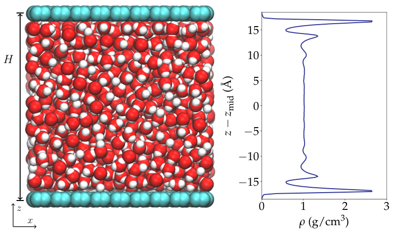
Water confined between two parallel graphene sheets is studied with molecular dynamics simulations using the Large-scale Atomic/Molecular Massively Parallel Simulator (LAMMPS) Plimpton 1995. The size of the simulation box is Å, where is defined as the distance between the centers of the carbon atoms in opposing graphene sheets. Periodic boundary conditions are applied in the and direction, whilst the direction remains fixed to avoid interactions of water molecules across boundaries. is varied between and Å in order to explore different states of confinement, from monolayer water to large separations where a significant bulk region is recovered at the center of the channel (see Fig. 1). For small separations, more finely spaced distances were examined, in order to observe the layering transition behavior of water. In order to calculate the fluid volume, an effective height of the channel, , is defined as , where Å is the Lennard-Jones characteristic distance for the carbon-oxygen interaction Werder et al. 2003. Consequently, the volume occupied by the fluid is given by . This definition of has been used in the literature Mosaddeghi et al. 2012 to best match the average density in the channel to the density of the bulk regions of water for large separations. The channel average density in all cases is g/cm3 in accordance with the bulk density of water. Additional simulations were performed at higher average channel densities. For each separation, three different starting configurations in terms of velocity seeds were probed.
Water is simulated using the SPC/E force field Berendsen et al. 1987. SPC/E is chosen over more accurate but more computationally expensive models, such as TIPP/2005 and TIPP/ICE, in order to balance accuracy in the determination of transport properties with the associated computational cost. The water-carbon interaction used in this work is parametrized using the SPC/E model Werder et al. 2003, a potential frequently used in water flow simulations Khademi and Sahimi 2011; Zhu et al. 2013; Wei et al. 2014; Sam et al. 2017. Previous studies have shown ice formation of monolayer SPC/E and TIPP/2005 models with the same lattice constant Algara-Siller et al. 2015, confirming the independence of these results with respect to the details of the force fields. The bonds and angles are constrained using the SHAKE algorithm Ryckaert et al. 1977. The carbon-water interaction parameters by Werder et al. Werder et al. 2003, optimized to reproduce the experimentally observed contact angle, are used, where eV and Å. The chosen cut-off radius is Å, with the PPPM method Rajagopal and Needs 1994 employed to evaluate long-range electrostatic interactions. The carbon atoms are uncharged and non-interacting. The graphene sheets consist of carbon atoms each, whilst the water phase comprises to molecules, depending on the channel separation, . In order to maintain a system temperature of K, an equilibration run of ns with a Nosé-Hoover thermostat Nosé 1984; Hoover 1985 applied to both the graphene sheets and the water molecules with a damping constant of 0.05 ps is performed. The thermostat is subsequently removed and temperature control was ensured by applying a Berendsen thermostat Berendsen et al. 1984 with a damping term of 100 ps to the graphene sheets only, allowing for the water dynamics to be observed unimpeded. The carbon atoms are tethered to their relative position with a spring constant of eV/Å2 to hold the sheet in place and allow for vibrations to dissipate energy. After a further equilibration period of ns in the microcanonical ensemble, a production run is performed for ns.
2.2 Green-Kubo methods for transport calculations
The velocity autocorrelation function (VACF) quantifies how strongly atom velocities at a certain time influence the velocities at later points. The normalized VACF is given by
| (1) |
where all fluid atoms are considered in the averaging. is the ensemble average of the correlation for different time origins. Here, the velocity vector in the two dimensions parallel to the graphene sheets is given by . The diffusion coefficient can be calculated using the mean-squared displacement (MSD), using
| (2) |
where the dimensionality is taken as so as to only take into account the MSD in the plane parallel to the graphene sheet. The slope of the MSD hence determines the diffusivity. Here, is the position vector corresponding to the velocity vector given above, i.e. .
The shear viscosity, , is related to the time autocorrelation function of the off-diagonal elements of the stress tensor, , with , and is as such a tensor. In a homogeneous system all elements of this tensor, , are equivalent and can be averaged in order to achieve more accurate results. However, in confinement this is not the case and the elements need to be carefully chosen for their validity. In this definition, is the direction of the velocity in shear flow, and the direction of displacement. Previous work Liu et al. 2005 has shown that calculating , where is the direction of confinement, produces unphysically low values. As such, only values of which are not the direction of the confinement are employed. We therefore calculate through
| (3) |
where is the fluid volume as defined before.
Additionally, the bulk viscosity, , of confined water is calculated. In an isotropic system with short vibrational relaxation times, as is the case for water, is calculated using the time autocorrelation function of the pressure. The question arises on how to apply this to a highly confined system. In the only known calculation of the bulk viscosity under confinement in the literature Goyal et al. 2013, the correlation function is not calculated directly but expressed as a phenomenological analytic equation as a function of relaxation times accounting for structural and dynamical contributions. Confinement is accounted for by modifying the dynamical relaxation time to include a dependence on the distance from the confining wall, which is integrated over. A solution more closely related to the original definition in terms of correlation functions is to consider confined water as a fluid, implying no expansion or dilation takes place in the direction. This allows us to define the instantaneous pressure as and calculate its correlation over time, such that is given by
| (4) |
where , and the ensemble average over time.
The viscosity autocorrelation functions are sampled every fs with a correlation length of ps.
2.3 Order parameter
In order to assess the formation and properties of the ice phases, the planar orientational order parameter, , can be calculated throughChaikin and Lubensky 1995; Das et al. 1999; Crane et al. 2008
| (5) |
Here, is the angle between the vectors of a sample atom and the nearest neighbours. Nearest neighbours are defined as being located at the first maximum of the oxygen-oxygen radial distribution function, . here takes the value 4, to define a measure of square order, where 1 is high and 0 indicates no order. The order parameter, , is evaluated in the -plane, only.
3 Results
3.1 Diffusivity and shear viscosity
The top panel of Fig. 2 shows the diffusion coefficient in the -plane as calculated using the MSD, where g/cm3. Between Å, the diffusion coefficient is up to orders of magnitude smaller than in the bulk. This sharp decrease points to a strong hindrance in the mobility. This is further supported by the shear viscosity, , in the plane parallel to the graphene surface as shown in the middle panel of Fig. 2 as a function of sheet separation. A sharp increase of the shear viscosity is seen for the same channel heights. Outside this region, whilst at large separations does approach the corresponding value for bulk water at the same density, it nevertheless remains higher at all separations, with some additional enhancement seen for separations of up to Å. For the largest separation examined here, Å, mPas, compared to the bulk value of mPas.
When the density is higher, the effect on transport properties is more significant. For instance, for a monolayer of water with g/cm3, the diffusion coefficient reaches values as low as m2/s, an order of magnitude lower than for g/cm3 (see Tabs. S2 and S3). Similarly, the shear viscosity is increased by an additional order of magnitude. The shear viscosity shows oscillatory behaviour for channel heights up to 16 Å.
3.2 Bulk viscosity
The bulk viscosity, , shows similar behaviour to , in that there is an increased value observed in confinement (bottom panel of Fig. 2). For large separations, approaches mPas, which is times larger than the corresponding bulk value, and hence a larger enhancement than recorded for . For Å, whilst an increase compared to larger separations is observed throughout, one separation, Å, presents as an outlier and shows the largest enhancement by almost a factor of .
Overall, the viscosity ratio, , is larger than in the bulk, with a limiting value of for large separations, compared to for bulk water (see Fig. S15). However, for Å, returns to bulk values. These results highlight that the bulk viscosity at moderate confinement is more strongly affected than the shear viscosity, whereas at small separations the properties of the latter are more perturbed.
3.3 Ice formation


Our analysis of the simulation snapshots shows that highly ordered monolayer structures form for certain channel heights at room temperature ( K) and bulk densities ( g/cm3). For very small distances ( Å), a liquid monolayer is observed. However, for Å, from now on termed the ‘frozen’ regime, ordered systems are found, the nature of which depends on the channel height (Figs. S2-S6).
For all separations in the frozen regime, a rhombic structure, also sometimes referred to as square or ‘square-like’ in the literature Algara-Siller et al. 2015; Sobrino Fernandez Mario et al. 2015, is observed. For smaller distances, the crystalline structure is flat ( Å), whereas for larger separations, a puckered phase is found ( Å). In Fig. 3 a sample ice configuration for Å is shown. As can be seen in Fig. 3(a), the ice phase is predominantly a puckered rhombic monolayer phase. The side view emphasizes the puckered nature of the formation, as highlighted by the colouring. No net polarization is present here, in accordance with previous studies Mosaddeghi et al. 2012; Zhao et al. 2014; Zhou et al. 2015; Sobrino Fernandez Mario et al. 2015; Yang et al. 2017. Fig. 3(b) shows the corresponding time-averaged oxygen density, , where the rhombic arrangement of the oxygen atoms is evident.
Additional studies of this system at higher densities have shown that highly ordered systems form at carbon-to-carbon distances of Å up to distances of Å (Figs. S8-S12). Notably, not only monolayer, but also bilayer ice structures form, with clear bilayer ice formation appearing at widths of Å. Here, a rhombic ice phase with AB stacking is found. For comparison, the molecular arrangement, density and pressure profiles of the same channel separation, Å, with densities and g/cm3 are plotted in Fig. 4 . In the g/cm3 case, the pressures tangential to the graphene sheets, , are of the order of GPa, comparable to the pressures in previous studies of ice phases in confinement. The pressures in the higher density system, however, are an order of magnitude larger. The corresponding density profiles are shown in Fig. 4(c). Here, the effect of the increase in the density is clear, with a change from a broadened monolayer to bilayer water. This particular case showcases the sharp morphological changes in the adsorbed solid that occur upon a perturbation in density and highlights the difficulty in mapping the thermodynamic phase to a given geometry.

3.4 Order parameter
Fig. 5(a) shows the square order parameter, , for small channel heights. A clear maximum in the frozen region is seen, indicating increased square order. However, the maximum value achieved is still well below 1, pointing towards a departure from perfect squares. This is in agreement with the appearance of rhombic (rather than square) ice.
In order to investigate the unexpected value of found at Å, the structure and thermodynamic state of water at this confinement is inspected more closely by varying the average density in the channel. Whilst at g/cm3 most of the molecules are part of a rhombic ice structure, a small bubble can also be observed in the monolayer (see Fig. S2). Analysis of the order parameter, , at this height (Fig. 5(b)) shows that for densities in the liquid range, is low with values of 0.15, whereas for higher densities, an ordered, square-like system is found (). The case with an average density of g/cm3 sits in the middle between the two regimes, indicating that the system undergoes a phase transition. At this global density the system is under strain and the normal pressure is negative, with large fluctuations associated with the inherent instability of the phases.
3.5 Radial distribution function
The two-dimensional oxygen-oxygen radial distribution functions, , in the plane parallel to the graphene sheets () for liquid ( Å) and frozen ( Å) monolayer water at K at an average water density of g/cm3 are shown in Fig. 6. The liquid monolayer , whilst it shows an additional peak at Å not present in bulk water, nevertheless converges to within less than Å. The ordered monolayer, on the other hand, shows persistent oscillations over the entire distance examined. The peak of the is at approximately the same position in both cases, at Å, an observation that is made for all channel heights, , regardless of ordering. In the crystalline case, a further small peak is found at Å, with a prominent peak at Å. is roughly equivalent to , whilst . This peak spacing is commensurate with a square lattice.
3.6 Velocity autocorrelation function
The velocity autocorrelation function (VACF) is a good indicator of long-range order. Fig. 7 shows the difference between the 2 VACF for a liquid monolayer ( Å) and an ice monolayer ( Å) for room temperature ( K) confined water with average channel densities of g/cm3. The oscillations in the VACF for the ice phase highlight the ordering, as the change in sign reflects the collisions on short time scales experienced by the water molecules. The VACF for Å, on the other hand, strongly resembles that of the bulk, though indications of higher ordering prevail here as well, as indicated by a deeper first minimum compared to the bulk. An investigation of the mean-squared displacement (MSD) in the -plane (Fig. 7, inset) shows results commensurate with this. The MSD of the liquid is of the order of Å2 during the production run, whereas that of the frozen phase is instead two orders of magnitude smaller and plateaus at long times. This highlights that there is very little motion of the water molecules here associated with the frozen phase over the course of the entire production run, confirming crystallization.
4 Discussion
The results presented in this work show a significant decrease in mobility of confined water at small channel heights, Å, when g/cm3, of several orders of magnitude when compared to bulk water. At large separations, and approach the values recorded for bulk SPC/E, though mobility in the plane is always decreased, regardless of the level of confinement. Similar results have been reported in the literature: a comparable study by Neek-Amal et al. Neek-Amal et al. 2016 showed strong oscillations in the shear viscosity, , akin to our higher density study, where oscillatory behaviour in the shear viscosity is also observed. At g/cm3, we find a single peak in at small channel heights instead, highlighting the sensitivity of the system to small changes in density and pressure.
To the authors’ knowledge the bulk viscosity in confinement has only been calculated once in the current literature Goyal et al. 2013. Notably, water is not studied and no information is given on the phase (fluid or solid) in strong confinement. Similar to the work by Goyal et al., we see an increase in the bulk viscosity when confinement reaches values of a few molecular diameters. A continuous drop in the viscosity ratio, , is also observed for small separations, indicating that the shear viscosity enhancement is much larger than that of the bulk viscosity in strong confinement. In this work, confinement of less than 3 molecular diameters is additionally studied, which is not covered by Goyal et al. Here, returns to smaller values and in turn increases.
In order to further understand the strongly impeded mobility of the water molecules at small channel heights, the phase of water at varying levels of confinement was studied. The results presented demonstrate the formation of ice phases for Å when g/cm3, where only a monolayer of water is accommodated between the graphene sheets. Notably, for smaller separations, Å, a liquid monolayer is observed. In the frozen regime, both flat ( Å) and puckered ( Å) rhombic ice phases with no net polarization are seen, with pressures in the GPa range.
These results are qualitatively consistent with previous research on confined water Zangi and Mark 2003; Zhao et al. 2014; Zhu et al. 2015; Yang et al. 2017, where puckered monolayer ice phases are reported for Å, with flat phases observed for smaller channel heights Zhu et al. 2015; Yang et al. 2017, as reported here. The stability of square and rhombic 2 ice in confinement at GPa pressures has been confirmed using highly accurate diffusion Monte Carlo simulations Chen et al. 2016. These authors used different methods, including different water force fields and computational approaches, to achieve qualitatively similar results. However, unlike some results presented in the literature Zhao et al. 2014; Yang et al. 2017; Zangi and Mark 2003; Zhu et al. 2015; Sobrino Fernandez Mario et al. 2015, we do not find bi- or trilayer solid structures at bulk densities. This, however, is consistent with other studies of SPC/E water Mosaddeghi et al. 2012; Algara-Siller et al. 2015; Gao et al. 2018, where only at high pressures and densities multilayer ices are reported.
The strongly impeded mobility is clearly linked to the phase transition and subsequent solidification of water at small channel heights. Whilst classical molecular dynamics simulations using the SPC/E force field are not as accurate as ab initio methods, solidification is nevertheless observed in simulations regardless of force field or methodology Chen et al. 2016, with differences mostly restricted to the crystal structure that forms. Results for the viscosity ratio further show that crystallization impacts shear and diffusive properties to a larger degree than the bulk viscosity, whilst in the liquid phase the bulk viscosity is more strongly affected by confinement. The investigation of the phase behaviour also allows for an explanation of the large increase in for Å. As the analysis of the order parameter at different densities shows, water undergoes a liquid-to-solid phase transition at g/cm3, where several phases co-exist. The resulting instability causes the bulk viscosity to increase in this scenario. Similar enhancements are seen for pure, bulk fluids in the vapor-liquid region Jaeger et al. 2018. Increasing the global density at the same channel height shifts the equilibrium to the solid phase and results in a less pronounced value of in fully frozen configurations. Whilst the investigations of the impact of on flow behaviour are beyond the scope of this work, the effects of phase instabilities on transport properties should be an important consideration in future work.
5 Conclusion
This study bench-marked the dependence of both water structure and transport on the level of confinement experienced by water enclosed between two graphene sheets at K and average channel densities of g/cm3.
The above discussion demonstrates that transport properties are strongly affected and mobility is impeded in confinement, particularly at nanoscale channel heights. The phase transition and subsequent crystallization of water can account for this phenomenon, where phase changes are accompanied with abrupt changes in the transport properties. Here, the diffusion coefficient and shear viscosity are orders of magnitude smaller and larger, respectively. The phase transition has a particular impact on the bulk viscosity, as highlighted by the strong enhancement found for Å, where the system is unstable.
These effects on the properties of water need to be taken into account when trying to optimize the design of nanoscale devices where graphene structures are used as scaffolds, e.g. membranes for water purifications. In particular, the instability of phases needs to be considered in the process and should be either avoided in order to ensure predictable transport behaviour or, on the other hand, could be appropriately exploited. The extreme pressures recorded in confinement can be explained from a molecular point of view Long et al. 2013 and have been suggested as plausible routes for enhancing chemical reactivity in nanopores Gubbins et al. 2018. Further, regulating the freezing or melting of water requires fine control of the thermodynamic state, namely the density and the pressure.
ables of numerical results for the transport properties.
Simulation snapshots at different channel heights.
Sample input files for molecular dynamics simulations.
References
- Corry (2008) Corry, B. Designing carbon nanotube membranes for efficient water desalination. J. Phys. Chem. B 2008, 112, 1427–34.
- Cohen-Tanugi and Grossman (2012) Cohen-Tanugi, D.; Grossman, J. C. Water desalination across nanoporous graphene. Nano Lett. 2012, 12, 3602–8.
- Wang and Karnik (2012) Wang, E. N.; Karnik, R. Water desalination: graphene cleans up water. Nat. Nanotechnol. 2012, 7, 552–4.
- Kou et al. (2014) Kou, J.; Zhou, X.; Lu, H.; Wu, F.; Fan, J. Graphyne as the membrane for water desalination. Nanoscale 2014, 6, 1865–70.
- An et al. (2017) An, S.; Joshi, B. N.; Lee, J.-G.; Lee, M. W.; Kim, Y. I.; Kim, M.-w.; Jo, H. S.; Yoon, S. S. A comprehensive review on wettability, desalination, and purification using graphene-based materials at water interfaces. Catal. Today 2017, 295, 14–25.
- Corry (2011) Corry, B. Water and ion transport through functionalised carbon nanotubes: implications for desalination technology. Energy Environ. Sci. 2011, 4, 751.
- He et al. (2013) He, Z.; Zhou, J.; Lu, X.; Corry, B. Bioinspired graphene nanopores with voltage-tunable ion selectivity for Na(+) and K(+). ACS nano 2013, 7, 10148–10157.
- Konatham et al. (2013) Konatham, D.; Yu, J.; Ho, T. A.; Striolo, A. Simulation insights for graphene-based water desalination membranes. Langmuir 2013, 29, 11884–11897.
- Chan et al. (2014) Chan, E. P.; Mulhearn, W. D.; Huang, Y.-R.; Lee, J.-H.; Lee, D.; Stafford, C. M. Tailoring the permselectivity of water desalination membranes via nanoparticle assembly. Langmuir 2014, 30, 611–616.
- Ball (2008) Ball, P. Water - An enduring mystery. Nature 2008, 452, 291–292.
- Stokely et al. (2008) Stokely, K.; Mazza, M. G.; Stanley, H. E.; Franzese, G. Effect of hydrogen bond cooperativity on the behavior of water. Proc. Natl. Acad. Sci. U.S.A. 2008, 107, 1301–1306.
- Nilsson and Pettersson (2015) Nilsson, A.; Pettersson, L. G. M. The structural origin of anomalous properties of liquid water. Nat. Commun. 2015, 6, 8998.
- Hummer et al. (2001) Hummer, G.; Rasaiah, J. C.; Noworyta, J. P. Water conduction through the hydrophobic channel of a carbon nanotube. Nature 2001, 414, 188–190.
- Kosztin et al. (2006) Kosztin, I.; Barz, B.; Janosi, L. Calculating potentials of mean force and diffusion coefficients from nonequilibrium processes without Jarzynski’s equality. J. Chem. Phys. 2006, 124, 64106.
- Bocquet and Charlaix (2010) Bocquet, L.; Charlaix, E. Nanofluidics, from bulk to interfaces. Chem. Soc. Rev. 2010, 39, 1073–1095.
- Wang et al. (2011) Wang, Y.; Zhao, Y. J.; Huang, J. P. Giant pumping of single-file water molecules in a carbon nanotube. J. Phys. Chem. B 2011, 115, 13275–9.
- Gravelle et al. (2014) Gravelle, S.; Joly, L.; Ybert, C.; Bocquet, L. Large permeabilities of hourglass nanopores: from hydrodynamics to single file transport. J. Chem. Phys. 2014, 526, 18C526.
- Majumder et al. (2005) Majumder, M.; Chopra, N.; Andrews, R.; Hinds, B. J. Enhanced flow in carbon nanotubes. Nature 2005, 438, 43–44.
- Holt et al. (2006) Holt, J. K.; Park, H. G.; Wang, Y.; Stadermann, M.; Artyukhin, A. B.; Grigoropoulos, C. P.; Noy, A.; Bakajin, O. Fast mass transport through sub-2-nanometer carbon nanotubes. Science 2006, 312, 1034–1037.
- Thomas and McGaughey (2009) Thomas, J. A.; McGaughey, A. J. H. Water flow in carbon nanotubes: transition to subcontinuum transport. Phys. Rev. Lett. 2009, 102, 1–4.
- Su and Guo (2012) Su, J.; Guo, H. Effect of nanochannel dimension on the transport of water molecules. J. Phys. Chem. B 2012, 116, 5925–5932.
- Suk and Aluru (2013) Suk, M. E.; Aluru, N. R. Molecular and continuum hydrodynamics in graphene nanopores. RSC Advances 2013, 3, 9365.
- Calabrò et al. (2013) Calabrò, F.; Lee, K. P.; Mattia, D. Modelling flow enhancement in nanochannels: viscosity and slippage. Appl. Math. Lett. 2013, 26, 991–994.
- Ritos et al. (2014) Ritos, K.; Mattia, D.; Calabrò, F.; Reese, J. M. Flow enhancement in nanotubes of different materials and lengths. J. Chem. Phys. 2014, 140, 014702.
- Mattia et al. (2015) Mattia, D.; Leese, H.; Lee, K. P. Carbon nanotube membranes: from flow enhancement to permeability. J. Membr. Sci. 2015, 475, 266–272.
- Kannam et al. (2017) Kannam, S. K.; Daivis, P. J.; Todd, B. D. Modeling slip and flow enhancement of water in carbon nanotubes. MRS Bull. 2017, 42, 283–288.
- Wang et al. (2017) Wang, Y.; Xu, J.; Wang, S.; Yang, C. Quantitative relationship between fluid inhomogeneities and flow enhancement in nanotubes. Nanoscale 2017, 9, 6777–6782.
- Gelb et al. (1999) Gelb, L. D.; Gubbins, K. E.; Radhakrishnan, R.; Sliwinska-Bartkowiak, M. Phase separation in confined systems. Rep. Prog. Phys. 1999, 62, 1573–1659.
- Koga et al. (2001) Koga, K.; Gao, G. T.; Tanaka, H.; Zeng, X. C. Formation of ordered ice nanotubes inside carbon nanotubes. Nature 2001, 412, 802–805.
- Koga et al. (2002) Koga, K.; Gao, G. T.; Tanaka, H.; Zeng, X. C. How does water freeze inside carbon nanotubes? Physica A 2002, 314, 462–469.
- Takaiwa et al. (2008) Takaiwa, D.; Hatano, I.; Koga, K.; Tanaka, H. Phase diagram of water in carbon nanotubes. Proc. Natl. Acad. Sci. U.S.A. 2008, 105, 39–43.
- Pugliese et al. (2017) Pugliese, P.; Conde, M. M.; Rovere, M.; Gallo, P. Freezing temperatures, ice nanotubes structures, and proton ordering of TIP4P/ICE water inside single wall carbon nanotubes. J. Phys. Chem. B 2017, 121, 10371–10381.
- Raju et al. (2018) Raju, M.; Van Duin, A.; Ihme, M. Phase transitions of ordered ice in graphene nanocapillaries and carbon nanotubes. Sci. Rep. 2018, 8, 1–11.
- Maniwa et al. (2005) Maniwa, Y.; Kataura, H.; Abe, M.; Udaka, A.; Suzuki, S.; Achiba, Y.; Kira, H.; Matsuda, K.; Kadowaki, H.; Okabe, Y. Ordered water inside carbon nanotubes: formation of pentagonal to octagonal ice-nanotubes. Chem. Phys. Lett. 2005, 401, 534–538.
- Agrawal et al. (2017) Agrawal, K. V.; Shimizu, S.; Drahushuk, L. W.; Kilcoyne, D.; Strano, M. S. Observation of extreme phase transition temperatures of water confined inside isolated carbon nanotubes. Nat. Nanotechnol. 2017, 12, 267–273.
- Zangi and Mark (2003) Zangi, R.; Mark, A. E. Monolayer ice. Phys. Rev. Lett. 2003, 91, 25502.
- Zangi and Mark (2003) Zangi, R.; Mark, A. E. Bilayer ice and alternate liquid phases of confined water. J. Chem. Phys. 2003, 119, 1694–1700.
- Zhao et al. (2014) Zhao, W. H.; Wang, L.; Bai, J.; Yuan, L. F.; Yang, J.; Zeng, X. C. Highly confined water: two-dimensional ice, amorphous ice, and clathrate hydrates. Acc. Chem. Res. 2014, 47, 2505–2513.
- Zhu et al. (2015) Zhu, Y. B.; Wang, F. C.; Bai, J.; Zeng, X. C.; Wu, H. A. Compression limit of two-dimensional water constrained in graphene nanocapillaries. ACS Nano 2015, 9, 12197–12204.
- Algara-Siller et al. (2015) Algara-Siller, G.; Lehtinen, O.; Wang, F. C.; Nair, R. R.; Kaiser, U.; Wu, H. A.; Geim, A. K.; Grigorieva, I. V. Square ice in graphene nanocapillaries. Nature 2015, 519, 443–5.
- Yang et al. (2017) Yang, L.; Guo, Y.; Diao, D. Structure and dynamics of water confined in a graphene nanochannel under gigapascal high pressure: dependence of friction on pressure and confinement. PCCP 2017, 19, 14048–14054.
- Mosaddeghi et al. (2012) Mosaddeghi, H.; Alavi, S.; Kowsari, M. H.; Najafi, B. Simulations of structural and dynamic anisotropy in nano-confined water between parallel graphite plates. J. Chem. Phys. 2012, 137.
- Zhou et al. (2015) Zhou, W.; Yin, K.; Wang, C.; Zhang, Y.; Xu, T.; Borisevich, A.; Sun, L.; Idrobo, J. C.; Chisholm, M. F.; Pantelides, S. T. et al. The observation of square ice in graphene questioned. Nature 2015, 528, E1–E2.
- Sobrino Fernandez Mario et al. (2015) Sobrino Fernandez Mario, M.; Neek-Amal, M.; Peeters, F. M. AA-stacked bilayer square ice between graphene layers. Phys. Rev. B 2015, 92, 1–5.
- Zheng et al. (2012) Zheng, Y.-g.; Ye, H.-f.; Zhang, Z.-q.; Zhang, H.-w. Water diffusion inside carbon nanotubes: mutual effects of surface and confinement. PCCP 2012, 14, 964–971.
- da Silva (2014) da Silva, L. B. Structural and dynamical properties of water confined in carbon nanotubes. J. Nanostructure Chem. 2014, 4, 104.
- Mashl et al. (2003) Mashl, R. J.; Joseph, S.; Aluru, N. R.; Jakobsson, E. Anomalously immobilized water: a new water phase induced by confinement in nanotubes. Nano Lett. 2003, 3, 589–592.
- Hirunsit and Balbuena (2007) Hirunsit, P.; Balbuena, P. B. Effects of confinement on water structure and dynamics: a molecular simulation study. J. Phys. Chem. C 2007, 111, 1709–1715.
- Neek-Amal et al. (2016) Neek-Amal, M.; Peeters, F. M.; Grigorieva, I. V.; Geim, A. K. Commensurability effects in viscosity of nanoconfined water. ACS Nano 2016, 10, 3685–3692.
- Myers (2011) Myers, T. G. Why are slip lengths so large in carbon nanotubes? Microfluid. Nanofluidics 2011, 10, 1141–1145.
- Thomas and McGaughey (2008) Thomas, J. A.; McGaughey, A. J. H. Reassessing fast water transport through carbon nanotubes. Nano Lett. 2008, 8, 2788–2793.
- Thomas et al. (2010) Thomas, J. A.; McGaughey, A. J. H.; Kuter-Arnebeck, O. Pressure-driven water flow through carbon nanotubes: insights from molecular dynamics simulation. Int. J. Therm. Sci. 2010, 49, 281–289.
- Mattia and Calabrò (2012) Mattia, D.; Calabrò, F. Explaining high flow rate of water in carbon nanotubes via solid-liquid molecular interactions. Microfluid. Nanofluidics 2012, 13, 125–130.
- Chen et al. (2008) Chen, X.; Cao, G.; Han, A.; Punyamurtula, V. K.; Liu, L.; Culligan, P. J.; Kim, T.; Qiao, Y. Nanoscale fluid transport: size and rate effects. Nano Lett. 2008, 8, 2988–2992.
- Babu and Sathian (2011) Babu, J. S.; Sathian, S. P. The role of activation energy and reduced viscosity on the enhancement of water flow through carbon nanotubes. J. Chem. Phys. 2011, 134.
- Ye et al. (2011) Ye, H.; Zhang, H.; Zhang, Z.; Zheng, Y. Size and temperature effects on the viscosity of water inside carbon nanotubes. Nanoscale Res. Lett. 2011, 6, 87.
- Zhang et al. (2011) Zhang, H.; Ye, H.; Zheng, Y.; Zhang, Z. Prediction of the viscosity of water confined in carbon nanotubes. Microfluid. Nanofluidics 2011, 10, 403–414.
- Köhler and Da Silva (2016) Köhler, M. H.; Da Silva, L. B. Size effects and the role of density on the viscosity of water confined in carbon nanotubes. Chem. Phys. Lett. 2016, 645, 38–41.
- Liu et al. (2016) Liu, B.; Wu, R.; Baimova, J. A.; Wu, H.; Law, A. W.-K.; Dmitriev, S. V.; Zhou, K. Molecular dynamics study of pressure-driven water transport through graphene bilayers. PCCP 2016, 18, 1886–1896.
- Fang et al. (2018) Fang, C.; Wu, X.; Yang, F.; Qiao, R. Flow of quasi-two dimensional water in graphene channels. J. Chem. Phys. 2018, 148.
- Tisza (1942) Tisza, L. Supersonic absorption and Stokes’ viscosity relation. Phys. Rev. 1942, 61, 531–536.
- Emanuel (1990) Emanuel, G. Bulk viscosity of a dilute polyatomic gas. Phys. Fluids A 1990, 2, 2252.
- Rah and Eu (2001) Rah, K.; Eu, B. C. Density and temperature dependence of the bulk viscosity of molecular liquids: Carbon dioxide and nitrogen. J. Chem. Phys. 2001, 114, 10436.
- Cramer (2012) Cramer, M. S. Numerical estimates for the bulk viscosity of ideal gases. Phys. Fluids 2012, 24, 066102.
- Li et al. (2017) Li, X.-D.; Hu, Z.-M.; Jiang, Z.-L. Continuum perspective of bulk viscosity in compressible fluids. J. Fluid. Mech. 2017, 812, 966–990.
- Jaeger et al. (2018) Jaeger, F.; Matar, O. K.; Müller, E. A. Bulk viscosity of molecular fluids. J. Chem. Phys. 2018, 148, 174504.
- Monchick et al. (1963) Monchick, L.; Yun, K. S.; Mason, E. A. Formal kinetic theory of transport phenomena in polyatomic gas mixtures. J. Chem. Phys. 1963, 39, 654.
- Prangsma et al. (1973) Prangsma, G. J.; Alberga, A. H.; Beenakker, J. J. M. Ultrasonic determination of the volume viscosity of N2, CO, CH4 and CD4 between 77 and 300 K. Physica 1973, 64, 278–288.
- Mayorga and Velasco (1997) Mayorga, M.; Velasco, R. M. Bulk viscosity of dilute molecular gases. Mol. Phys. 1997, 92, 49–54.
- Lin et al. (2017) Lin, J.; Scalo, C.; Hesselink, L. Bulk viscosity model for near-equilibrium acoustic wave attenuation. arXiv:1707.05876, 2017.
- Gray and Rice (1964) Gray, P.; Rice, S. A. On the kinetic theory of dense fluids. XVIII. The bulk viscosity. J. Chem. Phys. 1964, 41, 3689.
- Hanley and Cohen (1976) Hanley, H. J. M.; Cohen, E. G. D. Analysis of the transport coefficients for simple dense fluids : the diffusion and bulk viscosity coefficients. Physica 1976, 60, 215–232.
- Weyl (1949) Weyl, H. Shock waves in arbitrary fluids. Comm. Pure and Appl. Math. 1949, 2, 103–122.
- Gilbarg and Paolucci (1953) Gilbarg, D.; Paolucci, D. The structure of shock waves in the continuum theory of fluids. J. Rat. Mech. Anal. 1953, 2, 617–642.
- Emanuel (1998) Emanuel, G. Bulk viscosity in the Navier-Stokes equations. Int. J. Eng. Sci. 1998, 36, 1313–1323.
- Mani et al. (2009) Mani, A.; Larsson, J.; Moin, P. Suitability of artificial bulk viscosity for large-eddy simulation of turbulent flows with shocks. J. Comp. Phys. 2009, 228, 7368–7374.
- Emanuel (1992) Emanuel, G. Effect of bulk viscosity on a hypersonic boundary layer. Phys. Fluids A 1992, 4, 491–496.
- Billet et al. (2008) Billet, G.; Giovangigli, V.; de Gassowski, G. Impact of volume viscosity on a shock-hydrogen-bubble interaction. Comb. Theory Mod. 2008, 12, 221–248.
- Giovangigli (2015) Giovangigli, V. Multicomponent transport in laminar flames. Proc. Combust. Inst. 2015, 35, 625–637.
- Long et al. (2011) Long, Y.; Palmer, J. C.; Coasne, B.; Śliwinska-Bartkowiak, M.; Gubbins, K. E. Pressure enhancement in carbon nanopores: a major confinement effect. PCCP 2011, 13, 17163.
- Coasne et al. (2014) Coasne, B.; Long, Y.; Gubbins, K. E. Pressure effects in confined nanophases. Mol. Simul. 2014, 40, 721–730.
- Srivastava et al. (2017) Srivastava, D.; Santiso, E. E.; Gubbins, K. E. Pressure enhancement in confined fluids: effect of molecular shape and fluid-wall Interactions. Langmuir 2017, 33, 11231–11245.
- Srivastava et al. (2018) Srivastava, D.; Turner, C. H.; Santiso, E. E.; Gubbins, K. E. The Nitric Oxide dimer reaction in carbon nanopores. J. Phys. Chem. B 2018, 122, 3604–3614.
- Boretti et al. (2018) Boretti, A.; Al-Zubaidy, S.; Vaclavikova, M.; Al-Abri, M.; Castelletto, S.; Mikhalovsky, S. Outlook for graphene-based desalination membranes. npj Clean Water 2018, 1, 5.
- Seo et al. (2018) Seo, D. H.; Pineda, S.; Woo, Y. C.; Xie, M.; Murdock, A. T.; Ang, E. Y.; Jiao, Y.; Park, M. J.; Lim, S. I.; Lawn, M. et al. Anti-fouling graphene-based membranes for effective water desalination. Nat. Commun. 2018, 9, 1–12.
- Tabish et al. (2018) Tabish, T. A.; Memon, F. A.; Gomez, D. E.; Horsell, D. W.; Zhang, S. A facile synthesis of porous graphene for efficient water and wastewater treatment. Sci. Rep. 2018, 8, 1–14.
- Goyal et al. (2013) Goyal, I.; Zaheri, A. H. M.; Srivastava, S.; Tankeshwar, K. Longitudinal and volume viscosities of fluids confined in nanochannel. Phys. Chem. Liq. 2013, 51, 595–605.
- Plimpton (1995) Plimpton, S. Fast parallel algorithms for short-range molecular dynamics. J. Comp. Phys. 1995, 117, 1–19.
- Werder et al. (2003) Werder, T.; Walther, J.; Jaffe, R. L.; Halicioglu, T.; Koumoutsakos, P. On the water-carbon interaction for use in molecular dynamics simulations of graphite and carbon nanotubes. J. Phys. Chem. B 2003, 107, 1345–1352.
- Berendsen et al. (1987) Berendsen, H. J. C.; Grigera, J. R.; Straatsma, T. P. The missing term in effective pair potentials. J. Phys. Chem. 1987, 6269–6271.
- Khademi and Sahimi (2011) Khademi, M.; Sahimi, M. Molecular dynamics simulation of pressure-driven water flow in silicon-carbide nanotubes. J. Chem. Phys. 2011, 135.
- Zhu et al. (2013) Zhu, C.; Li, H.; Zeng, X. C.; Wang, E. G.; Meng, S. Quantized water transport: ideal desalination through graphyne-4 membrane. Sci. Rep. 2013, 3, 3163.
- Wei et al. (2014) Wei, N.; Peng, X.; Xu, Z. Understanding water permeation in graphene oxide membranes. ACS Appl. Mater. Interfaces 2014, 6, 5877–5883.
- Sam et al. (2017) Sam, A.; Kumar Kannam, S.; Hartkamp, R.; P. Sathian, S. Water flow in carbon nanotubes: the effect of tube flexibility and thermostat. J. Chem. Phys. 2017, 146, 234701.
- Ryckaert et al. (1977) Ryckaert, J. P.; Ciccotti, G.; Berendsen, H. J. C. Numerical integration of the cartesian equations of motion of a system with constraints: molecular dynamics of n-alkanes. J. Comp. Phys. 1977, 23, 327–341.
- Rajagopal and Needs (1994) Rajagopal, G.; Needs, R. J. An optimized Ewald method for long-ranged potentials. J. Comp. Phys. 1994, 115, 399–405.
- Nosé (1984) Nosé, S. A unified formulation of the constant temperature molecular dynamics methods. J. Chem. Phys. 1984, 81, 511–519.
- Hoover (1985) Hoover, W. G. Canonical dynamics: equilibrium phase-space distributions. Phys. Rev. A 1985, 31, 1695–1697.
- Berendsen et al. (1984) Berendsen, H. J. C.; Postma, J. P. M.; van Gunsteren, W. F.; DiNola, A.; Haak, J. R. Molecular dynamics with coupling to an external bath. J. Chem. Phys. 1984, 81, 3684–3690.
- Liu et al. (2005) Liu, Y.; Wang, Q.; Zhang, L.; Wu, T. Dynamics and density profile of water in nanotubes as one-dimensional fluid. Langmuir 2005, 21, 12025–12030.
- Chaikin and Lubensky (1995) Chaikin, P. M.; Lubensky, T. C. Principles of Condensed Matter Physics; Cambridge University Press, 1995.
- Das et al. (1999) Das, C.; Sood, A. K.; Krishnamurthy, H. R. Bond-orientational ordering and shear rigidity in modulated colloidal liquids. Physica A 1999, 270, 237–244.
- Crane et al. (2008) Crane, A. J.; Martínez-Veracoechea, F. J.; Escobedo, F. A.; Müller, E. A. Molecular dynamics simulation of the mesophase behaviour of a model bolaamphiphilic liquid crystal with a lateral flexible chain. Soft Matter 2008, 4, 1820–1829.
- Chen et al. (2016) Chen, J.; Zen, A.; Brandenburg, J. G.; Alfè, D.; Michaelides, A. Evidence for stable square ice from quantum Monte Carlo. Phys. Rev. B 2016, 94, 1–5.
- Gao et al. (2018) Gao, Z.; Giovambattista, N.; Sahin, O. Phase diagram of water confined by graphene. Sci. Rep. 2018, 8, 1–11.
- Long et al. (2013) Long, Y.; Palmer, J. C.; Coasne, B.; Śliwinska-Bartkowiak, M.; Jackson, G.; Müller, E. A.; Gubbins, K. E. On the molecular origin of high-pressure effects in nanoconfinement: the role of surface chemistry and roughness. J. Chem. Phys. 2013, 139.
- Gubbins et al. (2018) Gubbins, K. E.; Gu, K.; Huang, L.; Long, Y.; Mansell, J. M.; Santiso, E. E.; Shi, K.; Śliwińska-Bartkowiak, M.; Srivastava, D. Surface-driven high-pressure processing. Engineering 2018, 4, 311–320.