A Deterministic Gradient-Based Approach to Avoid Saddle Points

Lisa Maria Kreusser Affiliation: Department of Applied Mathematics and Theoretical Physics Affiliation: University of Cambridge Email: L.M.Kreusser@damtp.cam.ac.uk Stanley J. Osher Affiliation: Department of Mathematics Affiliation: University of California, Los Angeles Email: sjo@math.ucla.edu Bao Wang Affiliation: Department of Mathematics Affiliation: Scientific Computing and Imaging Institute Affiliation: University of Utah Email: wangbaonj@gmail.com

Abstract

Loss functions with a large number of saddle points are one of the major obstacles for training modern machine learning models efficiently. First-order methods such as gradient descent are usually the methods of choice for training machine learning models. However, these methods converge to saddle points for certain choices of initial guesses. In this paper, we propose a modification of the recently proposed Laplacian smoothing gradient descent [Osher et al., arXiv:1806.06317], called modified Laplacian smoothing gradient descent (mLSGD), and demonstrate its potential to avoid saddle points without sacrificing the convergence rate. Our analysis is based on the attraction region, formed by all starting points for which the considered numerical scheme converges to a saddle point. We investigate the attraction region’s dimension both analytically and numerically. For a canonical class of quadratic functions, we show that the dimension of the attraction region for mLSGD is $\left\lfloor(n-1)/2\right\rfloor$ , and hence it is significantly smaller than that of the gradient descent whose dimension is $n-1$ .

1 Introduction

Training machine learning (ML) models often reduces to solving the empirical risk minimization problem [30]

\min_{\mathbf{x}\in\mathbb{R}^{n}}f(\mathbf{x})

(1)

where $f\colon\mathbb{R}^{n}\to\mathbb{R}$ is the empirical risk functional, defined as

\displaystyle f(\mathbf{x}):=\frac{1}{N}\sum_{i=1}^{N}\mathcal{L}(\mathbf{y}_{i},g(\mathbf{d}_{i},\mathbf{x})).

Here, the training set $\{(\mathbf{d}_{i},\mathbf{y}_{i})\}_{i=1}^{N}$ with $\mathbf{d}_{i}\in\mathbb{R}^{n},\mathbf{y}_{i}\in\mathbb{R}^{m}$ for $n,m\in\mathbb{N}$ is given, $g\colon\mathbb{R}^{n}\times\mathbb{R}^{n}\to\mathbb{R}^{m}$ denotes the machine learning model parameterized by $\mathbf{x}$ and $\mathcal{L}(\mathbf{y}_{i},g(\mathbf{d}_{i},\mathbf{x}))$ is the training loss between the ground-truth label $\mathbf{y}_{i}\in\mathbb{R}^{m}$ and the model prediction $g(\mathbf{d}_{i},\mathbf{x})\in\mathbb{R}^{m}$ . The training loss function $\mathcal{L}$ is typically a cross-entropy loss for classification and a root mean squared error for regression. For many practical applications, $f$ is a highly nonconvex function, and $g$ is chosen among deep neural networks (DNNs), known for their remarkable performance across various applications. Deep neural network models are heavily overparametrized and require large amounts of training data. Both the number of samples $N$ and the dimension $n$ of $\mathbf{x}$ can scale up to millions or even billions [11, 27]. These complications pose serious computational challenges. Gradient descent (GD), stochastic gradient descent (SGD) and their momentum-accelerated variants are the method of choice for training high capacity ML models, since their merits include fast convergence, concurrence, and an easy implementation [2, 26, 32]. However, GD, or more generally first-order optimization algorithms relying only on gradient information, suffer from slow global convergence when saddle points exist [15].

Saddle points are omnipresent in high-dimensional nonconvex optimization problems, and correspond to highly suboptimal solutions of many machine learning models [6, 9, 10, 28]. Avoiding the convergence to saddle points and the escape from saddle points are two interesting mathematical problems. The convergence to saddle points can be avoided by changing the dynamics of the optimization algorithms in such a way that their iterates are less likely or do not converge to saddle points. Escaping from saddle points ensures that iterates close to saddle points escape from them efficiently. Many methods have recently been proposed for the escape from saddle points. These methods are either based on adding noise to gradients [7, 13, 14, 17] or leveraging high-order information, such as Hessian, Hessian-vector product or relaxed Hessian information [1, 3, 4, 5, 6, 19, 20, 22, 23, 25]. To the best of our knowledge, little work has been done in terms of avoiding saddle points with only first-order information.

GD is guaranteed to converge to first-order stationary points. However, it may get stuck at saddle points since only gradient information is leveraged. We call the region containing all starting points from which the gradient-based algorithm converges to a saddle point the attraction region. While it is known that the attraction region associated with any strict saddle points is of measure zero [15, 16] under GD for sufficiently small step sizes, it is still one of the major obstacles for GD to achieve fast global convergence; in particular, when there exist exponentially many saddle points [8]. This work aims to avoid saddle points by reducing the dimension of the attraction region and is motivated by the Laplacian smoothing gradient descent (LSGD) [24].

1.1 Our Contribution

We propose the first deterministic first-order algorithm for avoiding saddle points where no noisy gradients or any high-order information is required. We quantify the efficacy of the proposed new algorithm in avoiding saddle points for a class of canonical quadratic functions and extend the results to general quadratic functions. We summarize our major contributions below.

A small modification of LSGD

For solving minimization problems of the form (1), GD with initial guess $\mathbf{x}^{0}\in\mathbb{R}^{n}$ can be applied and resulting in the following GD iterates

\mathbf{x}^{k+1}=\mathbf{x}^{k}-\eta\nabla f(\mathbf{x}^{k}),

where $\eta>0$ denotes the step size. LSGD pre-multiplies the gradient by a Laplacian smoothing matrix with periodic boundary condition and leads to the following iterates

\mathbf{x}^{k+1}=\mathbf{x}^{k}-\eta\left(\mathbf{I}-\sigma\mathbf{L}\right)^{-1}\nabla f(\mathbf{x}^{k}),

where $\mathbf{I}$ is the $n\times n$ identity matrix and $\mathbf{L}$ is the discrete one-dimensional Laplacian, defined below in (4). LSGD can achieve significant improvements in training ML models [12, 24, 29], ML with differential privacy guarantees [31], federated learning [18], and Markov Chain Monte Carlo sampling [33].

In this work, we propose a small modification of LSGD to avoid saddle points efficiently. At its core is the replacement of the constant $\sigma$ in LSGD by an iteration-dependent function $\sigma(k)$ , resulting in the modified LSGD (mLSGD)

\displaystyle\mathbf{x}^{k+1}=\mathbf{x}^{k}-\eta\left(\mathbf{I}-\sigma(k)\mathbf{L}\right)^{-1}\nabla f(\mathbf{x}^{k}).

(2)

For the analysis, we assume that $\sigma(k)$ is a non-constant, monotonic function that is constant at some point. With such a small modification on LSGD, we show that mLSGD has the same convergence rate as GD and can avoid saddle points efficiently.

Quantifying the avoidance of saddle points

It is well-known that stochastic first-order methods like SGD rarely get stuck in saddle points, while standard first-order methods like GD may converge to saddle points. We show that small modifications of standard gradient-based methods such as mLSGD in (2) outperform GD in terms of saddle point avoidance due to its smaller attraction region. To quantify the set of initial data which leads to the convergence to saddle points, we investigate the dimension of the attraction region. Low-dimensional attraction regions are equivalent to high-dimensional subspaces of initial data which can avoid saddle points. Since many nonconvex optimization problems can locally be approximated by quadratic functions, we restrict ourselves to quadratic functions with saddle points in the following which also reduces additional technical difficulties arising with general functions. We consider the class of quadratic functions $f\colon\mathbb{R}^{n}\to\mathbb{R}$ with $f(\mathbf{x})=\frac{1}{2}\mathbf{x}^{T}\mathbf{B}\mathbf{x}$ where we assume that $\mathbf{B}$ has both positive and negative eigenvalues to guarantee the existence of saddle points. For different matrices $\mathbf{B}$ , our numerical experiments indicate that the dimension of the attraction region for the modified LSGD is a significantly smaller space than that for GD.

Analysing the dimension of the attraction region

For our analytical investigation of the avoidance of saddle points, we consider a canonical class of quadratic functions first, given by $f\colon\mathbb{R}^{n}\to\mathbb{R}$ with

f(x_{1},\cdots,x_{n})=\frac{c}{2}\left(\sum_{i=1}^{n-1}x_{i}^{2}-x_{n}^{2}\right)

(3)

with $c>0$ . The attraction regions of GD and the modified LSGD are given by

\mathcal{W}_{\text{GD}}=\left\{\mathbf{x}_{0}\in\mathbb{R}^{n}\colon\mathbf{x}^{k+1}=\mathbf{x}^{k}-\eta\nabla f(\mathbf{x}^{k})\text{ with }\lim_{k\to\infty}\mathbf{x}^{k}=\mathbf{0}\right\}

and

\mathcal{W}_{\text{mLSGD}}=\left\{\mathbf{x}_{0}\in\mathbb{R}^{n}\colon\mathbf{x}^{k+1}=\mathbf{x}^{k}-\eta\left(\mathbf{I}-\sigma(k)\mathbf{L}\right)^{-1}\nabla f(\mathbf{x}^{k})\text{ with }\lim_{k\to\infty}\mathbf{x}^{k}=\mathbf{0}\right\},

respectively, and are of dimensions

{\rm dim}\mathcal{W}_{\text{GD}}=n-1,\qquad{\rm dim}\mathcal{W}_{\text{mLSGD}}=\left\lfloor\frac{n-1}{2}\right\rfloor.

These results indicate that the set of initial data converging to a saddle point is significantly smaller for the modified LSGD than for GD. We extend these results to quadratic functions of the form $f(\mathbf{x})=\frac{1}{2}\mathbf{x}^{T}\mathbf{B}\mathbf{x}$ where $\mathbf{B}\in\mathbb{R}^{n\times n}$ has both positive and negative eigenvalues. In the two-dimensional case, the attraction region reduces to the trivial non-empty space $\{\mathbf{0}\}$ for most choices of $\mathbf{B}$ unless a very peculiar condition on eigenvectors of $\mathbf{B}$ is satisfied, implying that saddle points can be avoided for any starting point of the iterative method (2).

1.2 Notation

We use boldface upper-case letters $\mathbf{A}$ , $\mathbf{B}$ to denote matrices and boldface lower-case letters $\mathbf{x}$ , $\mathbf{y}$ to denote vectors. The vector of zeros of length $n$ is denoted by $\mathbf{0}\in\mathbb{R}^{n}$ and $A_{ij}$ denotes the entry $(i,j)$ of $\mathbf{A}$ . For vectors we use $\|\cdot\|$ to denote the Euclidean norm, and for matrices we use $\|\cdot\|$ to denote spectral norm, respectively. The eigenvalues of $\mathbf{A}$ are denoted by $\lambda_{i}(\mathbf{A})$ where we assume that they are ordered according to their real parts. For a function $f\colon\mathbb{R}^{n}\to\mathbb{R}$ , we use $\nabla f$ to denote its gradient.

1.3 Organization

This paper is structured as follows. In section 2, we revisit the LSGD algorithm and motivate the modified LSGD algorithm. For quadratic functions with saddle points, we rigorously prove in section 3 that the modified LSGD can significantly reduce the dimension of the attraction region. We provide a convergence analysis for the modified LSGD for nonconvex optimization in section 4. Furthermore, in section 5, we provide numerical results illustrating the avoidance of saddle points of the modified LSGD in comparison to the standard GD. Finally, we conclude.

2 Algorithm

2.1 LSGD

Recently, Osher et al. [24] proposed to replace the standard or stochastic gradient vector $\mathbf{y}\in\mathbb{R}^{n}$ by the Laplacian smoothed surrogate $\mathbf{A}_{\sigma}^{-1}\mathbf{y}\in\mathbb{R}^{n}$ where

\mathbf{A}_{\sigma}:=\mathbf{I}-\sigma\mathbf{L}=\begin{bmatrix}1+2\sigma&-\sigma&0&\dots&0&-\sigma\\ -\sigma&1+2\sigma&-\sigma&\dots&0&0\\ 0&-\sigma&1+2\sigma&\dots&0&0\\ \dots&\dots&\dots&\dots&\dots&\dots\\ -\sigma&0&0&\dots&-\sigma&1+2\sigma\end{bmatrix}

(4)

for a positive constant $\sigma$ , identity matrix $\mathbf{I}\in\mathbb{R}^{n\times n}$ and the discrete one-dimensional Laplacian $\mathbf{L}\in\mathbb{R}^{n\times n}$ . The resulting numerical scheme reads

\displaystyle\mathbf{x}^{k+1}=\mathbf{x}^{k}-\eta\mathbf{A}_{\sigma}^{-1}\nabla f(\mathbf{x}^{k}).

(5)

where GD is recovered for $\sigma=0$ . This simple Laplacian smoothing can help to avoid spurious minima, reduce the variance of SGD on-the-fly, and leads to better generalizations in training neural networks. Computationally, Laplacian smoothing can be implemented either by the Thomas algorithm together with the Sherman-Morrison formula in linear time, or by the fast Fourier transform (FFT) in quasi-linear time. For convenience, we use FFT to perform gradient smoothing where

\mathbf{A}_{\sigma}^{-1}\mathbf{y}={\rm ifft}\left(\frac{{\rm fft}(\mathbf{y})}{\mathbf{1}-\sigma\cdot{\rm fft}(\mathbf{d})}\right),

with $\mathbf{d}=[-2,1,0,\cdots,0,1]^{T}\in\mathbb{R}^{n}$ .

2.2 Motivation for modifying LSGD to avoid saddle points

To motivate the strength of modified LSGD methods in avoiding saddle points, we consider the two-dimensional setting, show the impact of varying $\sigma$ on the convergence to saddle points, and compare it to the convergence to saddle points for the standard LSGD with constant $\sigma$ .

2.2.1 Convergence to saddle points for LSGD

For given initial data $\mathbf{x}^{0}\in\mathbb{R}^{2}$ , we apply LSGD (5) for any constant $\sigma\geq 0$ to a quadratic function of the form $f(\mathbf{x})=\frac{1}{2}\mathbf{x}^{T}\mathbf{B}\mathbf{x}$ where we suppose that $\mathbf{B}\in\mathbb{R}^{2\times 2}$ has one positive and one negative eigenvalue for the existence of a saddle point. This yields

\displaystyle\mathbf{x}^{k+1}=\left(\mathbf{I}-\eta\mathbf{A}_{\sigma}^{-1}\mathbf{B}\right)\mathbf{x}^{k}=\left(\mathbf{I}-\eta\mathbf{A}_{\sigma}^{-1}\mathbf{B}\right)^{k+1}\mathbf{x}^{0}

(6)

where

\mathbf{A}_{\sigma}=\begin{bmatrix}1+\sigma&-\sigma\\ -\sigma&1+\sigma\end{bmatrix}.

Since $\mathbf{A}_{\sigma}^{-1}$ is positive definite, $\mathbf{A}_{\sigma}^{-1}\mathbf{B}$ has one positive and one negative eigenvalue, denoted by $\lambda_{+}$ and $\lambda_{-}$ , respectively. We write $\mathbf{p}_{+}$ and $\mathbf{p}_{-}$ for the associated eigenvectors and we have $\mathbf{x}^{0}=\alpha_{+}\mathbf{p}_{+}+\alpha_{-}\mathbf{p}_{-}$ for scalars $\alpha_{+},\alpha_{-}\in\mathbb{R}$ . This implies

\displaystyle\mathbf{x}^{k+1}=\alpha_{+}\left(1-\eta\lambda_{+}\right)^{k+1}\mathbf{p}_{+}+\alpha_{-}\left(1-\eta\lambda_{-}\right)^{k+1}\mathbf{p}_{-}.

If $\mathbf{x}^{0}\in\spann\{\mathbf{p}_{+}\}$ or, equivalently, $\alpha_{-}=0$ , we have $\lim_{k\to\infty}\mathbf{x}^{k}=\mathbf{0}$ for $\eta>0$ chosen sufficiently small such that $|1-\eta\lambda_{+}|<1$ is satisfied. Hence, we have convergence to the unique saddle point in this case.

Alternatively, we can study the convergence to the saddle point by considering the ordinary differential equation associated with (5). For this, we investigate the limit $\eta\to 0$ and obtain

\frac{\mathop{}\!\mathrm{d}\mathbf{x}}{\mathop{}\!\mathrm{d}t}=-\mathbf{A}_{\sigma}^{-1}\mathbf{B}\mathbf{x}

(7)

with initial data $\mathbf{x}(0)=\mathbf{x}^{0}$ . Since $\mathbf{x}^{0}=\alpha_{+}\mathbf{p}_{+}+\alpha_{-}\mathbf{p}_{-}$ for scalars $\alpha_{+},\alpha_{-}\in\mathbb{R}$ , the solution to (7) is given by

\mathbf{x}(t)=\alpha_{+}\mathbf{p}_{+}\exp{(-\lambda_{+}t)}+\alpha_{-}\mathbf{p}_{-}\exp{(-\lambda_{-}t)}.

If $\mathbf{x}^{0}\in\spann\{\mathbf{p}_{+}\}$ , the solution to (7) reduces to

\mathbf{x}(t)=\alpha_{+}\mathbf{p}_{+}\exp{(-\lambda_{+}t)}

and $\mathbf{x}(t)\to\mathbf{0}$ as $t\to\infty$ , i.e., LSGD for a constant $\sigma$ converges to the unique saddle point of $f$ .

This motivation can also be extended to the $n$ -dimensional setting. For that, we consider $f(\mathbf{x})=\frac{1}{2}\mathbf{x}^{T}\mathbf{B}\mathbf{x}$ where $\mathbf{B}\in\mathbb{R}^{n\times n}$ is a matrix with $k$ negative and $n-k$ positive eigenvalues. We assume that the eigenvalues are ordered, i.e. $\lambda_{1}\geq\ldots\geq\lambda_{n-k}>0>\lambda_{n-k+1}\geq\ldots\geq\lambda_{n}$ , and the associated eigenvectors are denoted by $\mathbf{p}_{1},\ldots,\mathbf{p}_{n}$ . One can easily show that for any starting point in $\spann\{p_{1},\ldots,p_{n-k}\}$ , we have convergence to the saddle point, implying that the attraction region for GD or the standard LSGD is given by $\mathcal{W}_{\text{LSGD}}=\spann\{p_{1},\ldots,p_{n-k}\}$ with $\dim\mathcal{W}_{\text{LSGD}}=n-k$ .

2.2.2 Avoidance of saddle points for the modified LSGD

In general, the eigenvectors and eigenvalues of $\mathbf{A}_{\sigma}^{-1}\mathbf{B}$ depend on $\sigma$ . Hence, the behavior of the iterates $\mathbf{x}^{k}$ in (5) and their convergence to saddle points becomes more complicated for time-dependent functions $\sigma$ due to the additional time-dependence of eigenvectors and eigenvalues. To illustrate the impact of a time-dependent $\sigma$ , we consider the special case $f(\mathbf{x})=\frac{1}{2}\mathbf{x}^{T}\mathbf{B}\mathbf{x}$ for

\mathbf{B}=\begin{bmatrix}1&0\\ 0&-1\end{bmatrix},

i.e., $f(\mathbf{x})=\frac{1}{2}(x_{1}^{2}-x_{2}^{2})$ for $\mathbf{x}=[x_{1},x_{2}]^{T}$ . The eigenvector $\mathbf{p}_{+}$ of $\mathbf{A}_{\sigma}^{-1}\mathbf{B}$ , associated with the positive eigenvalue $\lambda_{+}$ of $\mathbf{A}_{\sigma}^{-1}\mathbf{B}$ , is given by

\mathbf{p}_{+}=\begin{bmatrix}1\\ 0\end{bmatrix}\text{ for }\sigma=0\quad\text{ and }\quad\mathbf{p}_{+}=\frac{1}{\sqrt{\frac{(\sigma+1+\sqrt{2\sigma+1})^{2}+\sigma^{2}}{\sigma^{2}}}}\begin{bmatrix}\frac{\sigma+1+\sqrt{2\sigma+1}}{\sigma}\\ 1\end{bmatrix}\text{ for }\sigma>0.

It is easy to see that $\nu(\sigma)=\frac{\sigma+1+\sqrt{2\sigma+1}}{\sigma}$ is a strictly decreasing function in $\sigma$ with $\nu\to+\infty$ as $\sigma\to 0$ and $\nu\to 1$ as $\sigma\to\infty$ , implying that the corresponding normalised vector $\mathbf{p}_{+}$ is rotated counter-clockwise as $\sigma$ increases. Since $\mathbf{p}_{+}$ is given by $[\cos\phi,\sin\phi]^{T}$ for some $\phi\in[0,\frac{\pi}{4}]$ , this implies that for $\sigma_{1},\sigma_{2}$ with $\sigma_{1}\neq\sigma_{2}$ , the corresponding normalised eigenvectors $\mathbf{p}_{+}$ cannot be orthogonal and hence the associated normalised eigenvectors $\mathbf{p}_{-}$ cannot be orthogonal to each other. In particular, this is true for any bounded, strictly monotonic function $\sigma(k)$ of the iteration number $k$ . Figure 1 depicts the attraction regions for LSGD with constant values for $\sigma$ , given by $\sigma=0$ , $\sigma=10$ and $\sigma=100$ , respectively. Note that $\sigma=0$ corresponds to the standard gradient descent. Two attraction regions intersect only at the origin, indicating that starting from any point except $\mathbf{0}$ , LSGD results in a slight change of direction in every time step while $\sigma$ is strictly monotonic. This observation motivates that the modified LSGD for strictly monotonic $\sigma$ perturbs the gradient structure of $f$ in a non-uniform way while in the standard GD and LSGD the gradient is merely rescaled. In particular, the change of direction of the iterates in every time step motivates the avoidance of the saddle point $\mathbf{0}$ in the two-dimensional setting, while for LSGD with $\sigma$ constant, the iterates will converge to the saddle point for any starting point in $\spann\{\mathbf{p}_{+}\}$ .

Refer to caption — Figure 1: The attraction region when LSGD is applied to $f(\mathbf{x})=\frac{1}{2}(x_{1}^{2}-x_{2}^{2})$ . The black, blue and red lines are the corresponding attraction regions for $\sigma=0$ , $\sigma=10$ and $\sigma=100$ , , respectively.

2.3 Modified LSGD

Based on the above heuristics, we formulate the modified LSGD algorithm for positive, monotonic and bounded functions $\sigma(k)$ . The numerical scheme for the modified LSGD is given by

\mathbf{x}^{k+1}=\mathbf{x}^{k}-\eta\mathbf{A}_{\sigma(k)}^{-1}\nabla f(\mathbf{x}^{k})

(8)

where $\mathbf{A}_{\sigma(k)}=\mathbf{I}-\sigma(k)\mathbf{L}$ . The Laplacian smoothed surrogate $\mathbf{A}_{\sigma(k)}^{-1}\nabla f(\mathbf{x}^{k})$ can be computed by using either the Thomas algorithm or the FFT with the same computational complexity as the standard LSGD.

Remark 1.

For $\sigma(k)$ in the numerical scheme (8), we choose a positive function which is easy to compute. Any positive, strictly monotonic and bounded function $\sigma(k)$ guarantees the rotation of at least one eigenvector in the example in section 2.2.2.

3 Modified LSGD Can Avoid Saddle Points

In this section, we investigate the dimension of the attraction region for different classes of quadratic functions.

3.1 Specific class of functions

We consider the canonical class of quadratic functions in (3) on $\mathbb{R}^{n}$ which has a unique saddle point at $\mathbf{0}$ . Note that this class of functions can be written as $f(\mathbf{x})=\frac{c}{2}\mathbf{x}^{T}\mathbf{B}\mathbf{x}$ for some $c>0$ , where

\mathbf{B}=\begin{bmatrix}1&&&\\ &\ddots&\\ &&1&\\ &&&-1\end{bmatrix}\in\mathbb{R}^{n\times n}.

Since $c>0$ is a scaling factor which only influences the speed of convergence but not the direction of the updates, we can assume without loss of generality that $c=1$ in the following. Starting from some point $\mathbf{x}^{0}\in\mathbb{R}^{n}$ and a given function $\sigma(k)$ , we apply the modified LSGD to $f$ , resulting in the iterative scheme

\mathbf{x}^{k+1}=(\mathbf{I}-\eta\mathbf{A}_{\sigma(k)}^{-1}\mathbf{B})\mathbf{x}^{k},

(9)

where $\mathbf{A}_{\sigma(k)}$ is defined in (4) for the function $\sigma=\sigma(k)$ .

Lemma 1.

For any $k\in\mathbb{N}$ fixed, the matrix $\mathbf{A}_{\sigma(k)}^{-1}\mathbf{B}$ is diagonalizable, its eigenvectors form a basis of $\mathbb{R}^{n}$ and the eigenvalues of the matrix $\mathbf{A}_{\sigma(k)}^{-1}\mathbf{B}$ satisfy

\displaystyle 1\geq\lambda_{1}(\mathbf{A}_{\sigma(k)}^{-1}\mathbf{B})\geq\ldots\geq\lambda_{n-1}(\mathbf{A}_{\sigma(k)}^{-1}\mathbf{B})>0>\lambda_{n}(\mathbf{A}_{\sigma(k)}^{-1}\mathbf{B})\geq-1,

where $\lambda_{i}(\mathbf{A}_{\sigma(k)}^{-1}\mathbf{B})$ denotes the $i$ th largest eigenvalue of the matrix $\mathbf{A}_{\sigma(k)}^{-1}\mathbf{B}$ . In particular, $\mathbf{A}_{\sigma(k)}^{-1}\mathbf{B}$ has exactly one negative eigenvalue.

Proof.

For ease of notation, we denote $\sigma(k)$ by $\sigma$ in the following. As a first step, we show that $\mathbf{A}_{\sigma}^{-1}\mathbf{B}$ is diagonalizable and its eigenvalues $\lambda_{i}(\mathbf{A}_{\sigma}^{-1}\mathbf{B})$ are real for $i=1,\ldots,n$ . We prove this by showing that $\mathbf{A}_{\sigma}^{-1}\mathbf{B}$ is similar to a symmetric matrix. Note that $\mathbf{A}_{\sigma}^{-1}$ is a real, symmetric, positive definite matrix. Hence, $\mathbf{A}_{\sigma}^{-1}$ is diagonalizable with $\mathbf{A}_{\sigma}^{-1}=\mathbf{U}\mathbf{D}\mathbf{U}^{T}$ for an orthogonal matrix $\mathbf{U}$ and a diagonal matrix $\mathbf{D}$ with eigenvalues $\lambda_{i}(\mathbf{A}_{\sigma}^{-1})>0$ for $i=1,\ldots,n$ on the diagonal. This implies that there exists a real, symmetric, positive definite square root $\mathbf{A}_{\sigma}^{-1/2}=\mathbf{U}\sqrt{\mathbf{D}}\mathbf{U}^{T}$ with $\mathbf{A}_{\sigma}^{-1/2}\mathbf{A}_{\sigma}^{-1/2}=\mathbf{A}_{\sigma}^{-1}$ where $\sqrt{\mathbf{D}}$ denotes a diagonal matrix with diagonal entries $\sqrt{\lambda_{i}(\mathbf{A}_{\sigma}^{-1})}>0$ . We have

\mathbf{A}_{\sigma}^{1/2}\mathbf{A}_{\sigma}^{-1}\mathbf{B}\mathbf{A}_{\sigma}^{-1/2}=\mathbf{A}_{\sigma}^{-1/2}\mathbf{B}\mathbf{A}_{\sigma}^{-1/2}

where $\mathbf{A}_{\sigma}^{-1/2}\mathbf{B}\mathbf{A}_{\sigma}^{-1/2}$ is symmetric due to the symmetry of $\mathbf{A}_{\sigma}^{-1/2}$ and $\mathbf{B}$ . Thus, $\mathbf{A}_{\sigma}^{-1}\mathbf{B}$ is similar to the symmetric matrix $\mathbf{A}_{\sigma}^{-1/2}\mathbf{B}\mathbf{A}_{\sigma}^{-1/2}$ . In particular, $\mathbf{A}_{\sigma}^{-1}\mathbf{B}$ is diagonalizable and has real eigenvalues like $\mathbf{A}_{\sigma}^{-1/2}\mathbf{B}\mathbf{A}_{\sigma}^{-1/2}$ .

Note that $\det(\mathbf{A}_{\sigma}^{-1}\mathbf{B})=\det(\mathbf{A}_{\sigma}^{-1})\det(\mathbf{B})<0$ since $\det(\mathbf{A}_{\sigma}^{-1})>0$ and $\det(\mathbf{B})=-1$ . Since the determinant of a matrix is equal to the product of its eigenvalues and all eigenvalues of $\mathbf{A}_{\sigma}^{-1}\mathbf{B}$ are real, this implies that $\mathbf{A}_{\sigma}^{-1}\mathbf{B}$ has an odd number of negative eigenvalues. Next, we show that $\mathbf{A}_{\sigma}^{-1}\mathbf{B}$ has exactly one negative eigenvalue. Defining

\tilde{\mathbf{B}}:=\begin{pmatrix}0&&&\\ &\ddots&\\ &&0&\\ &&&-2\end{pmatrix}

we have

\mathbf{A}_{\sigma}^{-1}\mathbf{B}=\mathbf{A}_{\sigma}^{-1}+\mathbf{A}_{\sigma}^{-1}\tilde{\mathbf{B}}

where the matrix $\mathbf{A}_{\sigma}^{-1}\tilde{\mathbf{B}}$ has $n-1$ -fold eigenvalue 0 and its last eigenvalue is given by $-2[\mathbf{A}_{\sigma}^{-1}]_{nn}$ . We can write $\mathbf{A}_{\sigma}^{-1}=\frac{1}{\det\mathbf{A}_{\sigma}}\tilde{\mathbf{C}}$ where $\tilde{C}_{ij}=(-1)^{i+j}M_{ij}$ for the $(i,j)$ -minor $M_{ij}$ , defined as the determinant of the submatrix of $\mathbf{A}_{\sigma}$ by deleting the $i$ th row and the $j$ th column of $\mathbf{A}_{\sigma}$ . Since all leading principal minors are positive for positive definite matrices, this implies that $M_{nn}>0$ due to the positive definiteness of $\mathbf{A}_{\sigma}$ and hence $[\mathbf{A}_{\sigma}]_{nn}>0$ , implying that $\lambda_{i}(\mathbf{A}_{\sigma}^{-1}\tilde{\mathbf{B}})=0$ for $i=1,\ldots,n-1$ and $\lambda_{n}(\mathbf{A}_{\sigma}^{-1}\tilde{\mathbf{B}})<0$ . The eigenvalues of $\mathbf{A}_{\sigma}^{-1}\mathbf{B}$ can now be estimated by Weyl’s inequality for the sum of matrices, leading to

\lambda_{n-2}(\mathbf{A}_{\sigma}^{-1}\mathbf{B})\geq\lambda_{n-1}(\mathbf{A}_{\sigma}^{-1})+\lambda_{n-1}(\mathbf{A}_{\sigma}^{-1}\tilde{\mathbf{B}})>0

since the first term is positive and the second term is negative. Since $\mathbf{A}_{\sigma}^{-1}\mathbf{B}$ has an odd number of negative eigenvalues, this implies that $\lambda_{n-1}(\mathbf{A}_{\sigma}^{-1}\mathbf{B})>0$ and $\lambda_{n}(\mathbf{A}_{\sigma}^{-1}\mathbf{B})<0$ . In particular, $\mathbf{A}_{\sigma}^{-1}\mathbf{B}$ has exactly one negative eigenvalue.

To estimate upper and lower bounds of the eigenvalues of $\mathbf{A}_{\sigma}^{-1}\mathbf{B}$ , note that the eigenvalues of the Laplacian $L$ are given by $2-2\cos(2\pi k/n)\in[0,4]$ for $k=0,\ldots,n/2$ , implying that $\lambda_{i}(\mathbf{A}_{\sigma})\in[1,1+4\sigma]$ and in particular, we have

\lambda_{i}(\mathbf{A}_{\sigma}^{-1})\in\left[\frac{1}{1+4\sigma},1\right]

for $i=1,\ldots,n$ . Besides, we have

|\lambda_{i}(\mathbf{A}_{\sigma}^{-1}\mathbf{B})|\leq\rho(\mathbf{A}_{\sigma}^{-1}\mathbf{B})=\|\mathbf{A}_{\sigma}^{-1}\mathbf{B}\|\leq\|\mathbf{A}_{\sigma}^{-1}\|\|\mathbf{B}\|=\rho(\mathbf{A}_{\sigma}^{-1})\rho(\mathbf{B})\leq 1

all $i=1,\ldots,n$ , where $\rho(\mathbf{B})$ denotes the spectral radius of $\mathbf{B}$ and $\|\mathbf{B}\|$ denotes the operator norm of $\mathbf{B}$ . ∎

Since $\mathbf{A}_{\sigma(k)}^{-1}\mathbf{B}$ is diagonalizable by Lemma 1, we can consider the invertible matrix $\mathbf{P}_{\sigma(k)}=(\mathbf{p}_{1,\sigma(k)},\ldots,\mathbf{p}_{n,\sigma(k)})$ whose columns $\mathbf{p}_{i,\sigma(k)}$ denote the normalized eigenvectors of $\mathbf{A}_{\sigma(k)}^{-1}\mathbf{B}$ , associated with the eigenvalues $\lambda_{i}(\mathbf{A}_{\sigma(k)}^{-1}\mathbf{B})$ , i.e.

\lambda_{i}(\mathbf{A}_{\sigma(k)}^{-1}\mathbf{B})\mathbf{p}_{i,\sigma(k)}=\mathbf{A}_{\sigma(k)}^{-1}\mathbf{B}\mathbf{p}_{i,\sigma(k)}

for all $i=1,\ldots,n$ , and $\{\mathbf{p}_{1,\sigma(k)},\ldots,\mathbf{p}_{n,\sigma(k)}\}$ forms a basis of unit vectors of $\mathbb{R}^{n}$ . In the following, $p_{i,j,\sigma(k)}$ denotes the $i$ th entry of the $j$ th eigenvector $\mathbf{p}_{j,\sigma(k)}$ of $\mathbf{A}_{\sigma(k)}^{-1}\mathbf{B}$ , i.e. $\mathbf{p}_{j,\sigma(k)}=(p_{1,j,\sigma(k)},\ldots,p_{n,j,\sigma(k)})$ .

Lemma 2.

For any $k\in\mathbb{N}$ fixed, the matrix $\mathbf{A}_{\sigma(k)}^{-1}\mathbf{B}$ has $n-1$ eigenvectors $\mathbf{p}_{j,\sigma(k)}$ associated with positive eigenvalues. Of these, $\lfloor n/2\rfloor$ have the same form where the $l$ th entry $p_{l,j,\sigma(k)}$ of the $j$ th eigenvector $\mathbf{p}_{j,\sigma(k)}$ satisfies

\displaystyle p_{l,j,\sigma(k)}\begin{cases}=p_{n-l,j,\sigma(k)},&l=1,\ldots,n-1,\\ \neq 0,&l=n.\end{cases}

For the remaining $\lfloor(n-1)/2\rfloor$ eigenvectors associated with positive eigenvalues, the entry $p_{l,j,\sigma(k)}$ of eigenvector $\mathbf{p}_{j,\sigma(k)}$ satisfies

\displaystyle p_{l,j,\sigma(k)}=b\sin(l\theta_{j}),\quad l=1,\ldots,n,

(10)

where $\theta_{j}=\frac{2\pi m_{j}}{n}$ for some $m_{j}\in\mathbb{Z}$ and $b\in\mathbb{R}\backslash\{0\}$ such that $\|\mathbf{p}_{j,\sigma(k)}\|=1$ , implying

\displaystyle p_{l,j,\sigma(k)}=\begin{cases}-p_{n-l,j,\sigma(k)},&l=1,\ldots,n-1,\\ 0,&l=n.\end{cases}

The eigenvector $\mathbf{p}_{n,\sigma(k)}$ associated with the unique negative eigenvalue $\lambda_{n}(\mathbf{A}^{-1}_{\sigma(k)}\mathbf{B})$ satisfies

\displaystyle p_{l,n,\sigma(k)}\begin{cases}=p_{n-l,n,\sigma(k)},&l=1,\ldots,n-1,\\ \neq 0,&l=n.\end{cases}

Proof.

Since $k\in\mathbb{N}$ is fixed, we consider $\sigma$ instead of $\sigma(k)$ throughout the proof. Besides, we simplify the notation by dropping the index $\sigma=\sigma(k)$ in the notation of the eigenvectors $\mathbf{p}_{j,\sigma(k)}=(p_{1,j,\sigma(k)},\ldots,p_{n,j,\sigma(k)})$ , and we write $\mathbf{p}_{j}=(p_{1,j},\ldots,p_{n,j})$ for $j=1,\ldots,n$ .

Since $\mathbf{A}_{\sigma}^{-1}\mathbf{B}$ and $\mathbf{B}\mathbf{A}_{\sigma}$ have the same eigenvectors and their eigenvalues are reciprocals, we can consider $\mathbf{B}\mathbf{A}_{\sigma}$ for determining the eigenvectors $\mathbf{p}_{j}$ for $j=1,\ldots,n$ . Note that the $n-1$ eigenvectors $\mathbf{p}_{j}$ of $\mathbf{B}\mathbf{A}_{\sigma}$ for $j=1,\ldots,n-1$ are associated with positive eigenvalues $\lambda_{j}(\mathbf{B}\mathbf{A}_{\sigma})$ of $\mathbf{B}\mathbf{A}_{\sigma}$ , while the eigenvector $\mathbf{p}_{n}$ is associated with the only negative eigenvalue $\lambda_{n}(\mathbf{B}\mathbf{A}_{\sigma})$ . By introducing a slack variable $p_{0,j}$ we rewrite the eigenequation for the $j$ th eigenvalue $\lambda_{j}(\mathbf{B}\mathbf{A}_{\sigma})$ , given by

(\mathbf{B}\mathbf{A}_{\sigma}-\lambda_{j}(\mathbf{B}\mathbf{A}_{\sigma}))\mathbf{p}_{j}=\mathbf{0},

\displaystyle-\sigma p_{k-1,j}+(1+2\sigma-\lambda_{j}(\mathbf{B}\mathbf{A}))p_{k,j}-\sigma p_{k+1,j}=0,\quad k=1,\ldots,n-1,

(11)

with boundary conditions

\sigma p_{1,j}+\sigma p_{n-1,j}-(1+2\sigma+\lambda_{j}(\mathbf{B}\mathbf{A}_{\sigma}))p_{n,j}=0

(12)

and

p_{0,j}=p_{n,j}.

(13)

Equation (11) is a difference equation which can be solved by making the ansatz $p_{k,j}=r^{k}$ . Plugging this ansatz into (11) results in the quadratic equation

1-\frac{1+2\sigma-\lambda_{j}(\mathbf{B}\mathbf{A}_{\sigma})}{\sigma}r+r^{2}=0

with solutions $r_{+/-}=d\pm\sqrt{d^{2}-1}$ where

d:=\frac{1+2\sigma-\lambda_{j}(\mathbf{B}\mathbf{A}_{\sigma})}{2\sigma}.

Note that $r_{+}r_{-}=d^{2}-(d^{2}-1)=1$ and $2d=r_{+}+r_{-}=r_{+}+(r_{+})^{-1}$ .

Let us consider the eigenvector $\mathbf{p}_{n}$ first. Since $\lambda_{n}(\mathbf{B}\mathbf{A}_{\sigma})<0$ , this yields $d>1$ and in particular $r_{+}\neq r_{-}$ . We set $r:=r_{+}$ , implying $r_{-}=1/r$ , and obtain the general solution of the form

p_{k,n}=b_{1}r^{k}+b_{2}r^{-k},\quad k=0,\ldots,n

for scalars $b_{1},b_{2}\in\mathbb{R}$ which have to be determined from the boundary conditions (12),(13). From (13) we obtain

b_{1}+b_{2}=b_{1}r^{n}+b_{2}r^{-n},

implying that $b_{1}(1-r^{n})=b_{2}r^{-n}(1-r^{n})$ and in particular $b_{1}=b_{2}r^{-n}$ since $r=r_{+}>1$ . Hence, we obtain

p_{k,n}=b_{1}(r^{k}+r^{n-k}),\quad k=0,\ldots,n.

(14)

For non-trivial solutions for the eigenvector $\mathbf{p}_{n}$ we require $b_{1}\neq 0$ . Note that (14) implies that $p_{k,n}=p_{n-k,n}$ for $k=0,\ldots,n$ . It follows from boundary condition (12) that $p_{n,n}\neq 0$ is necessary for non-trivial solutions.

Next, we consider the $n-1$ eigenvectors $\mathbf{p}_{j}$ of $\mathbf{B}\mathbf{A}_{\sigma}$ associated with positive eigenvalues $\lambda_{j}(\mathbf{B}\mathbf{A}_{\sigma})>0$ for $j=1,\ldots,n-1$ . Note that all positive eigenvalues of $\mathbf{B}\mathbf{A}_{\sigma}$ are in the interval $[1,1+4\sigma]$ since $\lambda_{j}(\mathbf{A}_{\sigma})\in[1,1+4\sigma]$ and

\lambda_{j}(\mathbf{B}\mathbf{A}_{\sigma})=\frac{1}{\lambda_{j}(\mathbf{A}_{\sigma}^{-1}\mathbf{B})}\geq 1

by Lemma 1. Hence, $\lambda_{j}(\mathbf{B}\mathbf{A}_{\sigma})\leq\rho(\mathbf{B}\mathbf{A}_{\sigma})=\|\mathbf{B}\mathbf{A}_{\sigma}\|\leq\|\mathbf{B}\|\|\mathbf{A}_{\sigma}\|=\rho(\mathbf{B})\rho(\mathbf{A}_{\sigma})\leq 1+4\sigma$ . Thus, it is sufficient to consider three different cases $\lambda_{j}(\mathbf{B}\mathbf{A}_{\sigma})=1$ , $\lambda_{j}(\mathbf{B}\mathbf{A}_{\sigma})=1+4\sigma$ and $\lambda_{j}(\mathbf{B}\mathbf{A}_{\sigma})\in(1,1+4\sigma)$ .

We start by showing that all eigenvalues satisfy in fact $\lambda_{j}(\mathbf{B}\mathbf{A}_{\sigma})\in(1,1+4\sigma)$ . For this, assume that there exists $\lambda_{j}(\mathbf{B}\mathbf{A}_{\sigma})=1$ for some $j\in\{1,\ldots,n-1\}$ , implying that we have a single root $r_{+}=r_{-}=d=1$ . The general solution to the difference equation (11) with boundary conditions (12), (13) reads

p_{k,j}=(b_{1,j}+b_{2,j}k)r^{k}=b_{1,j}+b_{2,j}k,\quad k=0,\ldots,n

for constants $b_{1,j},b_{2,j}\in\mathbb{R}$ . Summing up all equations in (11) and subtracting (12) implies that $2p_{n,j}=0$ , i.e. $p_{n,j}=0$ . Hence, (13) implies $p_{0,j}=p_{n,j}$ and our ansatz yields $0=p_{n,j}=p_{0,j}=b_{1,j}$ . This results in $p_{k,j}=b_{2,j}k$ and $p_{n,j}=0=b_{2,j}n$ implies $b_{2,j}=0$ . In particular, there exists no non-trivial solution and $\lambda_{j}(\mathbf{B}\mathbf{A}_{\sigma})\neq 1$ for all $j=1,\ldots,n-1$ . Next, we show that $\lambda_{j}(\mathbf{B}\mathbf{A}_{\sigma})\neq 1+4\sigma$ for all $j=1,\ldots,n-1$ by contradiction. We assume that there exists $j\in\{1,\ldots,n-1\}$ such that $\lambda_{j}(\mathbf{B}\mathbf{A}_{\sigma})=1+4\sigma$ , implying that $r_{+}=r_{-}=d=-1$ . Due to the single root, the general solution is of the form

\displaystyle p_{k,j}=(b_{1,j}+b_{2,j}k)r^{k}=(b_{1,j}+b_{2,j}k)(-1)^{k},\quad k=0,\ldots,n.

For $n$ even, (13) yields $b_{1,j}=p_{0,j}=p_{n,j}=b_{1,j}+b_{2,j}n$ , implying $b_{2,j}=0$ . Hence, the solution is constant with $p_{k,j}=b_{1,j}$ , but does not satisfy boundary condition (12) unless $b_{1,j}=0$ , resulting in the trivial solution. Similarly, we obtain for $n$ odd that $b_{1,j}=p_{0,j}=p_{n,j}=-b_{1,j}-b_{2,j}n$ , implying $b_{2,j}=-2b_{1,j}/n$ , i.e. $p_{k,j}=b_{1,j}(1-2k/n)(-1)^{k}$ . Plugging this into the boundary condition (12) yields $b_{1,j}=0$ since $\sigma>0$ and $n\geq 2$ . In particular, there exists no non-trivial solution and the positive eigenvalues satisfy $\lambda_{j}(\mathbf{B}\mathbf{A}_{\sigma})<1+4\sigma$ for all $j=1,\ldots,n-1$ . Hence, we can now assume that $\lambda_{j}(\mathbf{B}\mathbf{A}_{\sigma})\in(1,1+4\sigma)$ . We conclude that $d\in(-1,1)$ and $r_{+/-}=d\pm i\sqrt{1-d^{2}}$ has two distinct roots. Setting $r:=r_{+}$ with $|r|=1$ , we can introduce an angle $\theta$ and write $r=\exp(i\theta)=\cos\theta+i\sin\theta$ , implying $d=\cos\theta$ and $r^{k}=\exp(ik\theta)$ . Due to the distinct roots we consider the ansatz

p_{k,j}=b_{1,j}r^{k}+b_{2,j}r^{-k},\quad k=0,\ldots,n.

The boundary condition (13) implies $b_{1,j}r^{n}(1-r^{n})=b_{2,j}(1-r^{n})$ resulting in the two cases $r^{n}=1$ and $b_{1,j}r^{n}=b_{2,j}$ .

For the case $r^{n}=\cos(n\theta)+i\sin(n\theta)=1$ , we conclude that $\theta=2\pi m/n$ for some $m\in\mathbb{Z}$ . This yields

	$\displaystyle p_{k,j}=(b_{1,j}+b_{2,j})\cos(k\theta)+i(b_{1,j}-b_{2,j})\sin(k\theta),$
	$\displaystyle\quad k=0,\ldots,n,$

and we obtain

	$\displaystyle p_{1,j}$	$\displaystyle=(b_{1,j}+b_{2,j})\cos(\theta)+i(b_{1,j}-b_{2,j})\sin(\theta),$
	$\displaystyle p_{n-1,j}$	$\displaystyle=(b_{1,j}+b_{2,j})\cos(\theta)-i(b_{1,j}-b_{2,j})\sin(\theta),$
	$\displaystyle p_{n,j}$	$\displaystyle=b_{1,j}+b_{2,j}.$

From boundary condition (12), we obtain

2\sigma(b_{1,j}+b_{2,j})\cos(\theta)-(1+2\sigma+\lambda_{j}(\mathbf{B}\mathbf{A}_{\sigma}))(b_{1,j}+b_{2,j})=0,

implying that $b_{1,j}+b_{2,j}=0$ or $2\sigma\cos(\theta)=1+2\sigma+\lambda_{j}(\mathbf{B}\mathbf{A}_{\sigma})$ . Since $\lambda_{j}(\mathbf{B}\mathbf{A}_{\sigma})>0$ , the second case cannot be satisfied and we conclude $b_{1,j}+b_{2,j}=0$ . This results in the general solution of the form $p_{k,j}=2ib_{1,j}\sin(k\theta)$ for $k=0,\ldots,n$ for $b_{1,j}\in\mathbb{C}$ , i.e., $\mathbf{p}_{j}=2ib_{1,j}(\sin(\theta),\ldots,\sin(n\theta))$ . Rescaling by $1/(2i)$ results in the real eigenvectors $\mathbf{p}_{j}=(p_{1,j},\ldots,p_{n,j})$ whose entries are of the form (10) where $b\in\mathbb{R}$ is chosen such that $\|\mathbf{p}_{j}\|=1$ . Here, $p_{k,j}=-p_{n-k,j}$ for $k=1,\ldots,n-1$ and $p_{n,j}=0$ . Further note that $p_{n/2,j}=0$ for $n$ even. By writing $\theta$ as $\theta_{j}=(2\pi m_{j})/n$ for some $m_{j}\in\mathbb{Z}$ , we can construct $(n-1)/2$ linearly independent eigenvectors for $n$ odd and $(n-2)/2$ for $n$ even, resulting in $\lfloor(n-1)/2\rfloor$ linearly independent eigenvectors for any $n\in\mathbb{N}$ . Since the matrix $\mathbf{A}_{\sigma}^{-1}\mathbf{B}$ is diagonalizable, there exist exactly $\lfloor(n-1)/2\rfloor$ normalized eigenvectors of the form (10).

For $b_{1,j}r^{n}=b_{2,j}$ , we obtain

p_{k,j}=b_{1,j}(r^{k}+r^{n-k})=p_{n-k,j},\quad k=0,\ldots,n,

i.e. the entries of $\mathbf{p}_{j}$ are arranged in the same way as the entries of $\mathbf{p}_{n}$ . Further note that we can always set $p_{n,j}\neq 0$ , and additionally $p_{k,j}$ with $k=1,\ldots,n/2$ for $n$ even and $p_{k,j}$ with $k=1,\ldots,(n-1)/2$ for $n$ odd, resulting in a space of dimension $\lfloor n/2\rfloor+1$ . Since $\mathbf{p}_{1},\ldots,\mathbf{p}_{n}$ form a basis of $\mathbb{R}^{n}$ , there are $\lfloor n/2\rfloor$ eigenvectors of this form, associated with positive eigenvalues. ∎

Lemma 2 implies that the matrix $\mathbf{A}_{\sigma(k)}^{-1}\mathbf{B}$ has one eigenvector $\mathbf{p}_{n,\sigma(k)}$ associated with the unique negative eigenvalue, $\lfloor(n-1)/2\rfloor$ eigenvectors of the form (10) and $\lfloor n/2\rfloor$ eigenvalues associated with certain positive eigenvalues which are of the same form as $\mathbf{p}_{n,\sigma(k)}$ . Note that $1+\lfloor(n-1)/2\rfloor+\lfloor n/2\rfloor=n$ for any $n\in\mathbb{N}$ .

In the following, we number the eigenvectors as follows. By $\mathbf{p}_{j,\sigma(k)}$ for $j=1,\ldots,\lfloor(n-1)/2\rfloor$ we denote the $\lfloor(n-1)/2\rfloor$ eigenvectors of the form (10). By $\mathbf{p}_{j,\sigma(k)}$ for $j=\lfloor(n-1)/2\rfloor+1,\ldots,n-1$ , we denote the $\lfloor n/2\rfloor$ eigenvectors of the form $p_{l,j,\sigma(k)}=p_{n-l,j,\sigma(k)}$ for $l=1,\ldots,n-1$ and $j=\lfloor(n-1)/2\rfloor+1,\ldots,n-1$ . The eigenvectors $\mathbf{p}_{j,\sigma(k)}$ for $j=1,\ldots,n-1$ , are associated with positive eigenvalues, and $\mathbf{p}_{n,\sigma(k)}$ denotes the eigenvector associated with the unique negative eigenvalue. Similarly, we relabel the eigenvalues so that eigenvalue $\lambda_{j}(\mathbf{A}_{\sigma(k)}^{-1}\mathbf{B})$ is associated with eigenvector $\mathbf{p}_{j,\sigma(k)}$ . Using this basis of eigenvectors, we can write $\mathbb{R}^{n}=\mathcal{V}\oplus\mathcal{W}$ with

\displaystyle\begin{split}\mathcal{V}:&=\left\{x_{k}=x_{n-k},k=1,\ldots,\left\lfloor\frac{n-1}{2}\right\rfloor\right\},\\ \mathcal{W}:&=\left\{x_{k}=-x_{n-k},k=1,\ldots,\left\lfloor\frac{n-1}{2}\right\rfloor;x_{n}=0\right\}.\end{split}

(15)

The spaces $\mathcal{V},\mathcal{W}$ satisfy

\displaystyle\mathcal{V}=\spann\{\mathbf{p}_{\lfloor(n-1)/2\rfloor+1,\sigma(k)},\ldots,\mathbf{p}_{n,\sigma(k)}\},\quad\mathcal{W}=\spann\{\mathbf{p}_{1,\sigma(k)},\ldots,\mathbf{p}_{\lfloor(n-1)/2\rfloor,\sigma(k)}\},

where $\mathcal{V}$ , $\mathcal{W}$ are orthogonal spaces and their definition is independent of $\sigma=\sigma(k)$ for any $k\in\mathbb{N}$ . For ease of notation, we introduce the set of indices $\mathcal{I}_{\mathcal{V}}:=\{\lfloor(n-1)/2\rfloor+1,\ldots,n\}$ and $\mathcal{I}_{\mathcal{W}}:=\{1,\ldots,\lfloor(n-1)/2\rfloor\}$ so that for all $k\in\mathbb{N}$ we obtain $\mathbf{p}_{i,\sigma(k)}\in\mathcal{V}$ for all $i\in\mathcal{I}_{\mathcal{V}}$ and $\mathbf{p}_{i,\sigma(k)}\in\mathcal{W}$ for all $i\in\mathcal{I}_{\mathcal{W}}$ . In particular, $\mathbf{p}_{i,\sigma(k)}$ for $i\in\mathcal{I}_{\mathcal{W}}$ is independent of $\sigma$ .

Remark 2 (Property of $\mathbf{p}_{n,\sigma(k)}$ ).

It follows immediately from the proof of Lemma 2 that $\mathbf{p}_{n,\sigma}$ can be computed for any $\sigma\geq 0$ . For $\sigma=0$ , we have $\mathbf{p}_{n,0}=[0,\ldots,0,1]^{T}$ since $\mathbf{A}_{0}=\mathbf{I}$ . For $\sigma>0$ , the $k$ th entry of $\mathbf{p}_{n,\sigma}$ is given by $p_{k,n,\sigma}=b_{1}(r^{k}+r^{n-k})$ for $k=1,\ldots,n$ , by (14), where the scalars $r>0$ and $b_{1}\in\mathbb{R}^{n}\backslash\{0\}$ depend on $\sigma$ . Since all entries of $p_{n}$ are positive if $b_{1}>0$ and negative if $b_{1}<0$ , this implies that for any $\sigma(k),\sigma(l)$ with $\sigma(k)\neq\sigma(l)$ , we have $\mathbf{p}_{n,\sigma(k)}\cdot\mathbf{p}_{n,\sigma(l)}\neq 0$ , i.e. the eigenvectors $\mathbf{p}_{n,\sigma(k)},\mathbf{p}_{n,\sigma(l)}$ are not orthonormal to each other. Since any $\mathbf{y}\in\mathcal{V}$ can be written as a linear combination of $\mathbf{p}_{j,\sigma(k)}$ for $j\in\mathcal{I}_{\mathcal{V}}$ , there exist $\beta_{j}$ for $j\in\mathcal{I}_{\mathcal{V}}$ with $\beta_{n}\neq 0$ such that $\mathbf{p}_{n,\sigma(l)}=\sum_{j\in\mathcal{I}_{\mathcal{V}}}\beta_{j}\mathbf{p}_{j,\sigma(k)}$ .

We have all the preliminary results to proof the main statement of this paper now:

Theorem 1.

Suppose that there exists $k_{0}>n-\lfloor(n-1)/2\rfloor$ such that $\sigma(k)=\sigma(k_{0})$ for all $k\geq k_{0}$ . For any $n\geq 2$ and $\mathbf{x}^{0}\notin\mathcal{W}\backslash\{0\}$ , the modified LSGD scheme (9) converges to the minimizer of $f$ . The attraction region $\mathcal{W}$ satisfies (15) and is of dimension $\lfloor(n-1)/2\rfloor$ .

Proof.

Let $\mathbf{x}^{0}\notin\mathcal{W}\backslash\{0\}$ and let $k\in\mathbb{N}$ be given. We write $\mathbf{x}^{k}=\sum_{i=1}^{n}\alpha_{i,k}\mathbf{p}_{i,\sigma(k)}$ as $\mathbf{x}^{k}=\mathbf{w}^{k}+\mathbf{v}^{k}$ where

\displaystyle\mathbf{v}^{k}:=\sum_{j\in\mathcal{I}_{\mathcal{V}}}\alpha_{j,k}\mathbf{p}_{j,\sigma(k)}\in\mathcal{V},\quad\mathbf{w}^{k}:=\sum_{j\in\mathcal{I}_{\mathcal{W}}}\alpha_{j,k}\mathbf{p}_{j,\sigma(k)}\in\mathcal{W}.

Here, $\mathcal{V},\mathcal{W}$ , defined in (15), are independent of $\sigma$ with $\mathbb{R}^{n}=\mathcal{V}\oplus\mathcal{W}$ . We apply the modified LSGD scheme (9) and consider the sequence $\mathbf{x}^{k+1}=(\mathbf{I}-\eta\mathbf{A}_{\sigma(k)}^{-1}\mathbf{B})\mathbf{x}^{k}=(\mathbf{I}-\eta\mathbf{A}_{\sigma(k)}^{-1}\mathbf{B})\mathbf{w}^{k}+(\mathbf{I}-\eta\mathbf{A}_{\sigma(k)}^{-1}\mathbf{B})\mathbf{v}^{k}$ . We define $\mathbf{w}^{k+1}=(\mathbf{I}-\eta\mathbf{A}_{\sigma(k)}^{-1}\mathbf{B})\mathbf{w}^{k}\in\mathcal{W}$ and $\mathbf{v}^{k+1}=(\mathbf{I}-\eta\mathbf{A}_{\sigma(k)}^{-1}\mathbf{B})\mathbf{v}^{k}\in\mathcal{V}$ iteratively. Since $\mathbf{p}_{j,\sigma(k)}$ and the associated eigenvalues $\lambda_{j}(\mathbf{A}^{-1}_{\sigma(k)}\mathbf{B})$ are in fact independent of $\sigma(k)$ for $j\in\mathcal{I}_{\mathcal{W}}$ , we have $\mathbf{p}_{j,\sigma(k+l)}=\mathbf{p}_{j,\sigma(k)}$ for any $l\geq 0$ . We obtain

\displaystyle\mathbf{w}^{k+l}

\displaystyle=\left(\prod_{j=1}^{l}(\mathbf{I}-\eta\mathbf{A}_{\sigma(k+j)}^{-1}\mathbf{B})\right)\mathbf{w}^{k}=\sum_{j\in\mathcal{I}_{\mathcal{W}}}\alpha_{j,k}(1-\eta\lambda_{j}(\mathbf{A}_{\sigma(k)}^{-1}\mathbf{B}))^{l}\mathbf{p}_{j,\sigma(k)}

for any $l\geq 0$ . By Lemma 1, the eigenvalues $\lambda_{j}(\mathbf{A}^{-1}_{\sigma(k)}\mathbf{B})$ satisfy $1-\eta\lambda_{j}(\mathbf{A}^{-1}_{\sigma(k)}\mathbf{B})\in(0,1)$ for $j\in\mathcal{I}_{\mathcal{W}}$ and any $\eta\in(0,1)$ , implying $\mathbf{w}^{k}\to 0$ as $k\to\infty$ . For proving the unboundedness of $\mathbf{x}^{k}$ as $k\to\infty$ it is hence sufficient to show that $\mathbf{v}^{k}$ is unbounded as $k\to\infty$ for any $\mathbf{v}^{0}\in\mathcal{V}\backslash\{0\}$ . Since $\sigma=\sigma(k)$ is constant for all $k\geq k_{0}$ , we have

\displaystyle\mathbf{v}^{k_{0}+l}

\displaystyle=\left(\prod_{j=1}^{l}(\mathbf{I}-\eta\mathbf{A}_{\sigma(k_{0}+j)}^{-1}\mathbf{B})\right)\mathbf{v}^{k_{0}}=\sum_{j\in\mathcal{I}_{\mathcal{V}}}\alpha_{j,k_{0}}(1-\eta\lambda_{j}(\mathbf{A}_{\sigma(k_{0})}^{-1}\mathbf{B}))^{l}\mathbf{p}_{j,\sigma(k_{0})}

for any $l\geq 0$ . Since $|1-\eta\lambda_{j}(\mathbf{A}_{\sigma(k_{0})}^{-1}\mathbf{B})|<1$ for $\eta\in(0,1)$ and all $j=1,\ldots,n-1$ , and $|1-\eta\lambda_{n}(\mathbf{A}_{\sigma(k_{0})}^{-1}\mathbf{B})|>1$ by Lemma 1, $\mathbf{v}^{k_{0}+l}$ is unbounded as $l\to\infty$ if and only if $\alpha_{n,k_{0}}\neq 0$ . We show that starting from $\mathbf{v}^{0}\in\mathcal{V}\backslash\{0\}$ there exists $k\geq 0$ such that ${\mathbf{v}}^{k}=\sum_{i\in\mathcal{I}_{\mathcal{V}}}\alpha_{i,k}\mathbf{p}_{i,\sigma(k)}\in\mathcal{V}\backslash\{\mathbf{0}\}$ with $\alpha_{n,k}\neq 0$ and by Remark 2 this guarantees $\alpha_{n,l}\neq 0$ for all $l\geq k$ .

Starting from $\mathbf{v}^{0}=\sum_{i\in\mathcal{I}_{\mathcal{V}}}\alpha_{i,0}\mathbf{p}_{i,\sigma(0)}\neq\mathbf{0}$ we can assume that $\alpha_{n,0}=0$ . Note that $\mathbf{v}^{0}$ is a function of $|\mathcal{I}_{\mathcal{V}}|=n-\lfloor(n-1)/2\rfloor$ parameters where one of the parameter in the linear combination can be regarded as a scaling parameter and thus, it can be set as any constant. This results in $n-\lfloor(n-1)/2\rfloor-2$ parameters which can be adjusted in such a way that $\mathbf{v}^{k}=\sum_{i\in\mathcal{I}_{\mathcal{V}}}\alpha_{i,k}\mathbf{p}_{i,\sigma(k)}$ with $\alpha_{n,k}=0$ for $k=0,\ldots,k_{e}$ with $k_{e}=n-\lfloor(n-1)/2\rfloor-2$ . We can determine these $n-\lfloor(n-1)/2\rfloor-1$ parameters from $n-\lfloor(n-1)/2\rfloor-1$ conditions, resulting in a linear system of $n-\lfloor(n-1)/2\rfloor-1$ equations. However, the additional condition

\displaystyle\mathbf{v}^{k_{e}+1}

\displaystyle=\Pi_{i=0}^{k_{e}}(\mathbf{I}-\eta\mathbf{A}_{\sigma(i)}^{-1}\mathbf{B})\mathbf{v}^{0}=\sum_{i\in\mathcal{I}_{\mathcal{V}}}\alpha_{i,k_{e}+1}\mathbf{p}_{i,\sigma(k_{e})}

with $\alpha_{n,k_{e}+1}=0$ leads to the unique trivial solution of the full linear system of size $n-\lfloor(n-1)/2\rfloor$ , i.e., the assumption $\mathbf{v}^{0}\neq\mathbf{0}$ is not satisfied. This implies that for any $\mathbf{v}^{0}\in\mathcal{V}\backslash\{0\}$ a vector $\mathbf{v}^{k}=\sum_{i\in\mathcal{I}_{\mathcal{V}}}\alpha_{i,k}\mathbf{p}_{i,\sigma(k)}$ with $\alpha_{n,k}\neq 0$ is reached in finitely (after at most $n-\lfloor(n-1)/2\rfloor-1$ ) steps. ∎

To sum up, in Theorem 1 we have discussed the convergence of the modified LSGD for the canonical class of quadratic functions in (3) on $\mathbb{R}^{n}$ . We showed:

•

The attraction region $\mathcal{W}$ of the modified LSGD is given by (15) with $\dim\mathcal{W}=\lfloor(n-1)/2\rfloor$ .
•

The definition of the attraction region $\mathcal{W}$ is given by the linear subspace of eigenvectors of $\mathbf{A}_{\sigma}^{-1}\mathbf{B}$ which are independent of $\sigma$ .
•

The attraction region of the modified LSGD is significantly smaller than for the attraction region $\mathcal{W}_{LSGD}$ of the standard GD or the standard LSGD with $\dim\mathcal{W}_{LSGD}=n-1$ .
•

For any $\mathbf{x}^{0}\notin\mathcal{W}$ , the modified LSGD scheme in (9) converges to the minimizer.
•

In the 2-dimensional setting, the attraction region of the modified LSGD satisfies $\mathcal{W}=\{0\}$ and is of dimension zero. For any $\mathbf{x}^{0}\neq\mathbf{0}$ the modified LSGD converges to the minimizer in this case.
•

The proof of Theorem 1 only considers the subspaces $\mathcal{V},\mathcal{W}$ and uses the independence of $\sigma$ of the eigenvectors in $\mathcal{W}$ . This observation is crucial for extending the results in Theorem 1 to any matrix $\mathbf{B}\in\mathbb{R}^{n\times n}$ with at least one positive and one negative eigenvalue.

3.2 Extension to quadratic functions with saddle points

While we investigated the convergence to saddle points for a canonical class of quadratic functions in Theorem 1, we consider quadratic functions of the form $f(\mathbf{x})=\frac{1}{2}\mathbf{x}^{T}\mathbf{B}\mathbf{x}$ for $\mathbf{B}\in\mathbb{R}^{n\times n}$ . First, we suppose that the saddle points of $f$ are non-degenerate, i.e., all eigenvalues of $\mathbf{B}\in\mathbb{R}^{n\times n}$ are non-zero. For the existence of saddle points, we require that there exist at least one positive and one negative eigenvalue of $\mathbf{B}$ .

Suppose that $\mathbf{B}$ has $k$ negative and $n-k$ positive eigenvalues. Since $\mathbf{A}_{\sigma}$ is positive definite for any $\sigma\geq 0$ , all its eigenvalues are positive and hence $\mathbf{A}_{\sigma}^{-1}\mathbf{B}$ has $k$ negative and $n-k$ positive eigenvalues. Due to the conclusion from Theorem 1, it is sufficient to determine the space $\mathcal{W}$ , consisting of all eigenvectors of $\mathbf{A}_{\sigma}^{-1}\mathbf{B}$ which are independent of $\sigma$ and are associated with positive eigenvalues.

Let $\sigma>0$ be given and suppose that $\mathbf{p}\in\mathcal{W}\backslash\{\mathbf{0}\}$ . Then, $\mathbf{p}$ is an eigenvector of $\mathbf{A}_{\sigma}^{-1}\mathbf{B}$ and $\mathbf{B}$ corresponding to eigenvalues $\lambda(\mathbf{A}_{\sigma}^{-1}\mathbf{B})>0$ and $\lambda(\mathbf{B})>0$ , respectively. By the definition of $\mathbf{p}$ , we have

\lambda(\mathbf{B})\mathbf{p}=\mathbf{B}\mathbf{p}=\lambda(\mathbf{A}_{\sigma}^{-1}\mathbf{B})\mathbf{A}_{\sigma}\mathbf{p}=\lambda(\mathbf{A}_{\sigma}^{-1}\mathbf{B})\mathbf{p}-\sigma\lambda(\mathbf{A}_{\sigma}^{-1}\mathbf{B})\mathbf{L}\mathbf{p}

where we used the definition of $\mathbf{A}_{\sigma}$ in (4). We conclude that $\mathbf{p}\in\mathcal{W}$ if and only if $\mathbf{L}\mathbf{p}\in\spann\{\mathbf{p}\}$ .

3.2.1 The 2-dimensional setting

For $n=2$ , the eigenvectors of $\mathbf{L}$ are given by

\displaystyle\mathbf{v}_{1}=\frac{1}{\sqrt{2}}\begin{bmatrix}1\\ 1\end{bmatrix},\qquad\mathbf{v}_{2}=\frac{1}{\sqrt{2}}\begin{bmatrix}1\\ -1\end{bmatrix},

associated with the eigenvalues $0$ and $-4$ , respectively. Since $\mathbf{p}\in\mathcal{W}$ can be written as $\mathbf{p}=\alpha_{1}\mathbf{v}_{1}+\alpha_{2}\mathbf{v}_{2}$ for coefficients $\alpha_{1},\alpha_{2}\in\mathbb{R}$ , we have $\mathbf{L}\mathbf{p}=-4\alpha_{2}\mathbf{v}_{2}$ . The condition $\mathbf{L}\mathbf{p}\in\spann\{p\}$ implies that $\mathbf{p}\in\spann\{\mathbf{v}_{1}\}$ or $\mathbf{p}\in\spann\{\mathbf{v}_{2}\}$ .

We require $\mathbf{B}\in\mathbb{R}^{2\times 2}$ has one positive and one negative eigenvalue for the existence of saddle points, i.e. $\mathbf{B}$ is diagonalisable. We conclude that $\dim\mathcal{W}=1$ if and only if

\displaystyle\mathbf{B}=\begin{bmatrix}\mathbf{v}&\mathbf{w}\end{bmatrix}\begin{bmatrix}\mu_{1}&0\\ 0&\mu_{2}\end{bmatrix}\begin{bmatrix}\mathbf{v}&\mathbf{w}\end{bmatrix}^{T}

where $\mu_{1}>0>\mu_{2}$ with $\mathbf{v}\in\spann\{\mathbf{v}_{1}\}$ or $\mathbf{v}\in\spann\{\mathbf{v}_{2}\}$ . Examples of matrices with $\dim\mathcal{W}=1$ include

\displaystyle\mathbf{B}_{1}=\begin{bmatrix}0&1\\ 1&0\end{bmatrix}\quad\text{and}\quad\mathbf{B}_{2}=\begin{bmatrix}0&-1\\ -1&0\end{bmatrix}

which correspond to the functions $f(\mathbf{x})=x_{1}x_{2}$ and $f(\mathbf{x})=-x_{1}x_{2}$ for $\mathbf{x}=[x_{1},x_{2}]^{T}$ , respectively. Since the eigenvector associated with the positive eigenvalue does not satisfy the above condition for most matrices $\mathbf{B}\in\mathbb{R}^{2\times 2}$ , we have $\dim\mathcal{W}=0$ for most $2$ -dimensional examples, including the canonical class discussed in Theorem 1.

3.2.2 The $n$ -dimensional setting

Similar to the proof in Lemma 1, one can show that the eigenvalues of the positive semi-definite matrix $-\mathbf{L}\in\mathbb{R}^{n\times n}$ have a specific form. We denote the $n$ eigenvalues of $\mathbf{L}$ by $\lambda_{1},\ldots,\lambda_{n}$ where $0=\lambda_{1}>\lambda_{2}\geq\ldots\geq\lambda_{n}$ with $\lambda_{2k}=\lambda_{2k+1}$ for $k=1,\ldots,\lfloor(n-1)/2\rfloor$ and $\lambda_{2k-1}>\lambda_{2k}$ for $k=1,\ldots,\lfloor n/2\rfloor$ . We denote by $\mathbf{v}_{i}$ the eigenvector associated with eigenvalue $\lambda_{i}$ of $\mathbf{L}$ .

To generalise the results in Theorem 1, we consider $\mathbf{B}\in\mathbb{R}^{n\times n}$ with $n-k$ positive eigenvalues and $k$ negative eigenvalues. We denote the eigenvectors associated with positive eigenvalues by $\mathbf{p}_{1},\ldots,\mathbf{p}_{n-k}$ and we have $\mathcal{W}\subset\spann\{\mathbf{p}_{1},\ldots,\mathbf{p}_{n-k}\}$ implying $\dim\mathcal{W}\leq n-k$ . In the worst case scenario, we have $\dim\mathcal{W}=n-k$ which is equal to the dimension of the attraction region of GD and the standard LSGD. However, only a small number of eigenvectors $\mathbf{p}_{j}$ for $j\in\{1,\ldots,n-k\}$ usually satisfies $\mathbf{L}\mathbf{p}_{j}\in\spann\{\mathbf{p}_{j}\}$ and hence $\dim\mathcal{W}$ is much smaller in practice. To see this, note that for any eigenvector $\mathbf{p}_{j}$ associated with a positive eigenvalue of $\mathbf{B}$ , we can write $\mathbf{p}_{j}=\sum_{i=1}^{n}\alpha_{i}\mathbf{v}_{i}$ for $\alpha_{1},\ldots,\alpha_{n}\in\mathbb{R}$ where $\mathbf{v}_{i}$ are the $n$ eigenvectors of $\mathbf{L}$ . Since $\mathbf{L}\mathbf{p}_{j}=\sum_{i=2}^{n}\alpha_{i}\lambda_{i}\mathbf{v}_{i}$ , we have $\mathbf{L}\mathbf{p}_{j}\in\spann\{\mathbf{p}_{j}\}$ if and only if $\mathbf{p}_{j}\in\spann\{\mathbf{v}_{1}\}$ or $\mathbf{p}_{j}\in\spann\{\mathbf{v}_{2k},\mathbf{v}_{2k+1}\}$ for some $k\in\{1,\ldots,\lfloor(n-1)/2\rfloor\}$ or, provided $n$ even, $\mathbf{p}_{j}\in\spann\{\mathbf{v}_{n}\}$ .

3.2.3 Degenerate Hessians

While our approach is very promising for Hessians with both positive and negative eigenvalues, it does not resolve issues of GD or LSGD related to degenerate saddle points where at least one eigenvalue is 0. Let $f(\mathbf{x})=\frac{1}{2}\mathbf{x}^{T}\mathbf{B}\mathbf{x}$ where $\mathbf{B}\in\mathbb{R}^{n\times n}$ has at least one eigenvalue 0 and let $\mathbf{p}$ denote an eigenvector associated with eigenvalue 0. Then, $\mathbf{A}_{\sigma}\mathbf{B}\mathbf{p}=\mathbf{0}$ for any $\sigma\geq 0$ and hence choosing $\mathbf{x}^{0}\in\spann\{\mathbf{p}\}$ as the starting point for the modified LSGD (9) will result in $\mathbf{x}^{k}=\mathbf{x}^{0}$ for all $k\geq 0$ like for GD and LSGD. The investigation of appropriate deterministic perturbations of first-order methods for saddle points where at least one eigenvalue is 0 is subject of future research.

4 Convergence Rate of the modified LSGD

In this section, we discuss the convergence rate of the modified LSGD for iteration-dependent functions $\sigma$ when applied to $\ell$ -smooth nonconvex functions $f\colon\mathbb{R}^{n}\to\mathbb{R}$ . Our analysis follows the standard convergence analysis framework. We start with the definitions of the smoothness of the objective function $f$ and a convergence criterion for nonconvex optimization.

Definition 1.

A differentiable function $f$ is $\ell$ -smooth (or $\ell$ -gradient Lipschitz), if for all $\mathbf{x},\mathbf{y}\in\mathbb{R}^{n}$ $f$ satisfies

f(\mathbf{y})\leq f(\mathbf{x})+\nabla f(\mathbf{x})\cdot(\mathbf{y}-\mathbf{x})+\frac{\ell}{2}\|\mathbf{x}-\mathbf{y}\|^{2}.

Definition 2.

For a differentiable function $f$ , we say that $\mathbf{x}$ is an $\epsilon$ -first-order stationary point if $\|\nabla f(\mathbf{x})\|\leq\epsilon$ .

Theorem 2.

Assume that the function $f$ is $\ell$ -smooth and let $\sigma$ be a positive, bounded function, i.e., there exists a constant $C>0$ such that $|\sigma(k)|\leq C$ for all $k\in\mathbb{N}$ . Then, the modified LSGD with $\sigma$ above, step size $\eta={1}/{\ell}$ and termination condition $\|\nabla f(\mathbf{x})\|\leq\epsilon$ converges to an $\epsilon$ -first-order stationary point within

\frac{2(1+4C)^{2}\ell(f(\mathbf{x}^{0})-f^{*})}{(1+8C)\epsilon^{2}}

iterations, where $f^{*}$ denotes a local minimum of $f$ .

Proof.

First, we will establish an estimate for $f(\mathbf{x}^{k+1})-f(\mathbf{x}^{k})$ for all $k\geq 0$ . By the $\ell$ -smoothness of $f$ and the LSGD scheme (9), we have

		$\displaystyle f(\mathbf{x}^{k+1})-f(\mathbf{x}^{k})$
		$\displaystyle\leq\langle\nabla f(\mathbf{x}^{k}),\left(\mathbf{x}^{k+1}-\mathbf{x}^{k}\right)\rangle+\frac{\ell}{2}\\|\mathbf{x}^{k+1}-\mathbf{x}^{k}\\|^{2}$
		$\displaystyle=\langle\nabla f(\mathbf{x}^{k}),-\frac{1}{\ell}\mathbf{A}_{\sigma(k)}^{-1}\nabla f(\mathbf{x}^{k})\rangle+\frac{1}{2\ell}\\|\mathbf{A}_{\sigma(k)}^{-1}\nabla f(\mathbf{x}^{k})\\|^{2}$
		$\displaystyle=\frac{1}{2\ell}\left\\|\left(\mathbf{A}_{\sigma(k)}^{-1}-\mathbf{I}\right)\nabla f(\mathbf{x}^{k})\right\\|^{2}-\frac{1}{2\ell}\\|\nabla f(\mathbf{x}^{k})\\|^{2}$
		$\displaystyle\leq\frac{1}{2\ell}\left\\|\mathbf{I}-\mathbf{A}_{\sigma(k)}^{-1}\right\\|^{2}\\|\nabla f(\mathbf{x}^{k})\\|^{2}-\frac{1}{2\ell}\\|\nabla f(\mathbf{x}^{k})\\|^{2}.$

To estimate $\|\mathbf{I}-\mathbf{A}_{\sigma(k)}^{-1}\|$ , we note that $\mathbf{A}_{\sigma(k)}^{-1}$ is diagonalizable, i.e., there exists an orthogonal matrix $\mathbf{Q}\in\mathbb{R}^{n\times n}$ and a diagonal matrix $\Lambda$ with diagonal entries $\lambda_{j}(\mathbf{A}_{\sigma(k)}^{-1})\in[1,1+4\sigma(k)]$ such that $\mathbf{A}_{\sigma(k)}^{-1}=\mathbf{Q}^{T}\boldsymbol{\Lambda}\mathbf{Q}$ . We have

\displaystyle\|\mathbf{I}-\mathbf{A}_{\sigma(k)}^{-1}\|^{2}=\|\mathbf{I}-\boldsymbol{\Lambda}\|^{2}\leq\left(1-\frac{1}{1+4\sigma(k)}\right)^{2}\leq\left(\frac{4C}{1+4C}\right)^{2}.

Plugging this estimate into the previous estimate yields

f(\mathbf{x}^{k+1})-f(\mathbf{x}^{k})\leq-\frac{1+8C}{2(1+4C)^{2}\ell}\|\nabla f(\mathbf{x}^{k})\|^{2}.

Based on the above estimate, the function value of the iterates decays by at least

\frac{1+8C}{2(1+4C)^{2}\ell}\|\nabla f(\mathbf{x}^{k})\|^{2}

in each iteration before an $\epsilon$ -first-order stationary point is reached. After

\frac{2(1+4C)^{2}\ell(f(\mathbf{x}^{0})-f^{*})}{(1+8C)\epsilon^{2}}

iterations, the modified LSGD is guaranteed to converge to an $\epsilon$ -first-order stationary point with function value $f^{*}$ .

∎

We note that the above convergence rate for nonconvex optimization is consistent with the gradient descent [21], and thus mLSGD converges as fast as GD.

5 Numerical Examples

In this section, we verify numerically that the modified LSGD does not converge to the unique saddle point in the two-dimensional setting, provided the matrices are not of the special case discussed in Section 3.2.1. We consider the bounded function $\sigma(k)=\frac{k+1}{k+2}$ for the modified LSGD. For both GD and the modified LSGD, we perform an exhaustive search with very fine grid sizes to confirm our theoretical results empirically. The exhaustive search is computationally expensive, and thus we restrict our numerical examples to the 2-dimensional setting.

5.1 Example 1

We consider the optimization problem

\min_{x_{1},x_{2}}f(x_{1},x_{2}):=x_{1}^{2}-x_{2}^{2}.

(16)

It is easy to see that $[0,0]^{T}$ is the unique saddle point of $f$ . We run $100$ iterations of GD and the modified LSGD with step size $\eta=0.1$ for solving (16). For GD, the attraction region is given by $\{[x_{1},x_{2}]^{T}\colon x_{1}\in\mathbb{R},x_{2}=0\}$ . To demonstrate GD’s behavior in terms of its convergence to saddle points, we start GD from any point in the set $\{[x_{1},x_{2}]^{T}\colon x_{1}=r\cos\theta,x_{2}=r\sin\theta,r\in[0.1,10],\theta\in[-1\text{e-6}^{\circ},1\text{e-6}^{\circ})\}$ , with a grid spacing of $0.1$ and $2\text{e-8}^{\circ}$ for $r$ and $\theta$ , respectively. As shown in Figure , the distance to the saddle point $[0,0]^{T}$ is 0 after 100 GD iterations for any starting point with $\theta=0$ . For starting points close to $[0,0]^{T}$ , given by small values of $r$ and any $\theta$ , the iterates are still very close to the saddle point after $100$ GD iterations with distances less than $0.1$ .

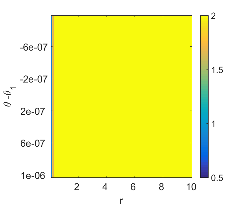
For the modified LSGD when applied to solve (16), the attraction region associated with the saddle point $[0,0]^{T}$ is of dimension zero, see Theorem 1. To verify this numerically, we consider any starting point in $\{[x_{1},x_{2}]^{T}|x_{1}=r\cos\theta,x_{2}=r\sin\theta,r\in[0.1,1],\theta\in[-180^{\circ},180^{\circ})\}$ with a grid spacing of $0.1$ and $1\text{e-6}^{\circ}$ for $r$ and $\theta$ , respectively. We observe that the minimum distance to $[0,0]^{T}$ is achieved when we start from the point $[r_{0}\cos\theta_{0},r_{0}\sin\theta_{0}]^{T}$ for $r_{0}=0.1$ and $\theta_{0}=166.8522^{\circ}$ . Then, we perform a finer grid search on the interval $[\theta_{0}-1^{\circ},\theta_{0}+1^{\circ}]$ using grid spacing $\Delta\theta=2\text{e-8}^{\circ}$ . This two-scale search significantly reduces the computational cost. Figure shows a similar region as in Figure , but with $\theta$ centered at $\theta_{0}$ . If $r=0.1$ , the distance to the saddle point is less than $0.3$ but larger than $0.2$ , implying that the distance to the saddle point increases by applying $100$ iterations of the modified LSGD. For any starting point with $r>0.1$ the distance is larger than $0.3$ after $100$ iterations. This illustrates that the iterates do not converge to the saddle point $[0,0]^{T}$ .

For the 2-dimensional setting, our numerical experiments demonstrate that the modified LSGD does not converge to the saddle point for any starting point provided the conditions in Section 3.2.1 are not satisfied. While there exists a region of starting points for GD with a slow escape from the saddle point, this region of slow escape is significantly smaller for the modified LSGD. These results are consistent with the dimension $\lfloor(n-1)/2\rfloor=0$ of the attraction region for the modified LSGD in Theorem 1. While the analysis is based on the assumption that $\sigma$ is constant at some point, the numerical results indicate that the theoretical results also hold for strictly monotonic, bounded functions $\sigma$ , provided $\sigma(k)$ for $k$ large enough is close to being stationary.

5.2 Example 2

To corroborate our theoretical findings numerically, we consider a two-dimensional problem where all entries of the coefficient matrix are non-zero. We consider

\min_{x_{1},x_{2}}f(x_{1},x_{2}):=x_{1}^{2}+6x_{1}x_{2}+2x_{2}^{2}

(17)

which satisfies $f(x_{1},x_{2})=\frac{1}{2}[x_{1}x_{2}]\mathbf{B}[x_{1}x_{2}]^{T}$ with

\displaystyle\mathbf{B}=\begin{bmatrix}2&6\\ 6&4\end{bmatrix}.

We apply GD with step size $\eta$ and starting from $[x_{1}^{0},x_{2}^{0}]^{T}$ for solving (17), resulting in the iterations

\displaystyle\begin{bmatrix}x_{1}^{k+1}\\ x_{2}^{k+1}\end{bmatrix}=\begin{bmatrix}x_{1}^{k}\\ x_{2}^{k}\end{bmatrix}-\eta\begin{bmatrix}2x_{1}^{k}+6x_{2}^{k}\\ 6x_{1}^{k}+4x_{2}^{k}\end{bmatrix}=\begin{bmatrix}x_{1}^{k}\\ x_{2}^{k}\end{bmatrix}+\eta\begin{bmatrix}-2&-6\\ -6&-4\end{bmatrix}\begin{bmatrix}x_{1}^{k}\\ x_{2}^{k}\end{bmatrix}.

(18)

The eigenvalues of the coefficient matrix $\mathbf{B}$ are $\lambda_{1}=\sqrt{37}+3$ and $\lambda_{2}=-\sqrt{37}+3$ , and the associated eigenvectors are

\displaystyle\mathbf{v}_{1}=\begin{bmatrix}\frac{\sqrt{37}-1}{6}\\ 1\end{bmatrix}\quad\text{and}\quad\mathbf{v}_{2}=\begin{bmatrix}\frac{-\sqrt{37}-1}{6}\\ 1\end{bmatrix},

respectively. If $[x_{1}^{0},x_{2}^{0}]^{T}$ is in $\spann\{\mathbf{v}_{1}\}$ , GD converges to the saddle point $[0,0]^{T}$ . As shown in Figure , starting from any point in $\spann\{[\cos\theta,\sin\theta]^{T}\}$ with

{\theta=\arctan\left(\frac{6}{\sqrt{37}-1}\right)},

$[x_{1}^{k},x_{2}^{k}]^{T}$ converges to the unique saddle point after 100 iteration. To corroborate our theoretical result that the modified LSGD does not converge to the saddle point in two dimensions, we perform a two-scale exhaustive search. First, we search over the initial point set $\{[x_{1},x_{2}]^{T}|x_{1}=r\cos\theta,x_{2}=r\sin\theta,r\in[0.1,1],\theta\in[-180^{\circ},180^{\circ})\}$ with grid spacing of $0.1$ and $1\text{e-6}^{\circ}$ for $r$ and $\theta$ , respectively. We observe that the minimum distance to $[0,0]^{T}$ is achieved when we start from the point $[r_{0}\cos\theta_{0},r_{0}\sin\theta_{0}]^{T}$ for $r_{0}=0.1$ and $\theta_{0}=-132.635976^{\circ}$ . Then, we perform a finer grid search on the interval $[\theta_{0}-1^{\circ},\theta_{0}+1^{\circ}]$ using the grid spacing $\Delta\theta=2\text{e-8}^{\circ}$ . Figure shows a similar region as in Figure , but with $\theta$ centered at $\theta_{0}$ . After $100$ LSGD iterations, the iterates do not converge to the saddle point $[0,0]^{T}$ , and we note that the minimum distance to the saddle point $[0,0]^{T}$ is $0.83$ .

6 Concluding Remarks

In this paper, we presented a simple modification of the Laplacian smoothing gradient descent (LSGD) to avoid saddle points. We showed that the modified LSGD can efficiently avoid saddle points both theoretically and empirically. In particular, we proved that the modified LSGD can significantly reduce the dimension of GD’s attraction region for a class of quadratic objective functions. Nevertheless, our current modified LSGD does not reduce the attraction region when applied to minimize some objective functions, e.g., $f(x_{1},x_{2})=x_{1}x_{2}$ . It is interesting to extend the idea of modified LSGD to avoid saddle points for general objective functions in the future.

To the best of our knowledge, our algorithm is the first deterministic gradient-based algorithm for avoiding saddle points that leverages only first-order information without any stochastic perturbation or noise. Our approach differs from existing perturbed or noisy gradient-based approaches for avoiding saddle points. It is of great interest to investigate the efficacy of a combination of these approaches in the future. A possible avenue is to integrate Laplacian smoothing with perturbed/noisy gradient descent to escape and circumvent saddle points more efficiently.

Acknowledgments

This material is based on research sponsored by the National Science Foundation under grant numbers DMS-1924935, DMS-1952339 and DMS-1554564 (STROBE), the Air Force Research Laboratory under grant numbers FA9550-18-0167 and MURI FA9550-18-1-0502, the Office of Naval Research under the grant number N00014-18-1-2527, and the Department of Energy under the grant number DE-SC0021142. LMK acknowledges support from the UK Engineering and Physical Sciences Research Council (EPSRC) grant EP/L016516/1, the German National Academic Foundation (Studienstiftung des Deutschen Volkes), the European Union Horizon 2020 research and innovation programmes under the Marie Skłodowska-Curie grant agreement No. 777826 (NoMADS) and No. 691070 (CHiPS), the Cantab Capital Institute for the Mathematics of Information and Magdalene College, Cambridge (Nevile Research Fellowship).

References

[1] N. Agarwal, Z. Allen-Zhu, B. Bullins, E. Hazan, and T. Ma, Finding Approximate Local Minima Faster than Gradient Descent, in Proceedings of the 49th Annual ACM SIGACT Symposium on Theory of Computing, STOC 2017, New York, NY, USA, 2017, Association for Computing Machinery, p. 1195–1199.
[2] Y. Bengio, Learning deep architectures for AI, Foundations and trends in Machine Learning, 2(1) (2009).
[3] Y. Carmon and J. C. Duchi, Gradient Descent Finds the Cubic-Regularized Nonconvex Newton Step, SIAM J. Optim., 29 (2019), pp. 2146–2178.
[4] F. E. Curtis and D. P. Robinson, Exploiting negative curvature in deterministic and stochastic optimization, Mathematical Programming, 176 (2019), pp. 69–94.
[5] F. E. Curtis, D. P. Robinson, and M. Samadi, A trust region algorithm with a worst-case iteration complexity of $\mathcal{O}(\epsilon^{-3/2})$ for nonconvex optimization, Mathematical Programming, (2014).
[6] Y. N. Dauphin, R. Pascanu, C. Gulcehre, K. Cho, S. Ganguli, and Y. Bengio, Identifying and attacking the saddle point problem in high-dimensional non-convex optimization, in Advances in Neural Information Processing Systems 27, Z. Ghahramani, M. Welling, C. Cortes, N. D. Lawrence, and K. Q. Weinberger, eds., Curran Associates, Inc., 2014, pp. 2933–2941.
[7] S. Du, C. Jin, J. D. Lee, M. I. Jordan, B. Poczos, and A. Singh, Gradient Descent Can Take Exponential Time to Escape Saddle Points, in Advances in Neural Information Processing Systems (NIPS 2017), 2017.
[8] R. Ge, Escaping from saddle points, 2016.
[9] R. Ge, F. Huang, C. Jin, and Y. Yuan, Escaping from saddle points — online stochastic gradient for tensor decomposition, in Proceedings of Machine Learning Research, P. Grünwald, E. Hazan, and S. Kale, eds., vol. 40, Paris, France, 03–06 Jul 2015, PMLR, pp. 797–842.
[10] R. Ge, F. Huang, C. Jin, and Y. Yuan, Escaping From Saddle Points – Online Stochastic Gradient for Tensor Decomposition, in Conference on Learning Theory (COLT 2015), 2015.
[11] K. He, X. Zhang, S. Ren, and J. Sun, Deep residual learning for image recognition, in Proceedings of the IEEE conference on computer vision and pattern recognition, 2016, pp. 770–778.
[12] M. Iqbal, M. A. Rehman, N. Iqbal, and Z. Iqbal, Effect of laplacian smoothing stochastic gradient descent with angular margin softmax loss on face recognition, in Intelligent Technologies and Applications, I. S. Bajwa, T. Sibalija, and D. N. A. Jawawi, eds., Singapore, 2020, Springer Singapore, pp. 549–561.
[13] C. Jin, R. Ge, P. Netrapalli, S. Kakade, and M. I. Jordan, How to Escape Saddle Points Efficiently, in Proceedings of the 34th International Conference on Machine Learning (ICML 2017), 2017.
[14] C. Jin, P. Netrapalli, and M. I. Jordan, Accelerated Gradient Descent Escapes Saddle Points Faster than Gradient Descent, in Conference on Learning Theory (COLT 2018), 2018.
[15] J. D. Lee, I. Panageas, G. Piliouras, M. Simchowitz, M. I. Jordan, and B. Recht, First-Order Methods Almost Always Avoid Strict Saddle Points, Math. Program., 176 (2019), p. 311–337.
[16] J. D. Lee, M. Simchowitz, M. I. Jordan, and B. Recht, Gradient Descent Only Converges to Minimizers, in Proceedings of Machine Learning Research, V. Feldman, A. Rakhlin, and O. Shamir, eds., vol. 49, Columbia University, New York, New York, USA, 23–26 Jun 2016, PMLR, pp. 1246–1257.
[17] K. Y. Levy, The power of normalization: Faster evasion of saddle points, arXiv:1611.04831, (2016).
[18] Z. Liang, B. Wang, Q. Gu, S. Osher, and Y. Yao, Exploring Private Federated Learning with Laplacian Smoothing, arXiv:2005.00218, (2020).
[19] M. Liu and T. Yang, On noisy negative curvature descent: Competing with gradient descent for faster non-convex optimization, arXiv:1709.08571, (2017).
[20] J. Martens, Deep Learning via Hessian-Free Optimization, in Proceedings of the 27th International Conference on International Conference on Machine Learning, ICML’10, Madison, WI, USA, 2010, Omnipress, p. 735–742.
[21] Y. Nesterov, Introductory lectures on convex programming volume I: Basic course, Lecture Notes, (1998).
[22] Y. Nesterov and B. T. Polyak, Cubic regularization of newton method and its global performance, Mathematical Programming, 108 (2006), pp. 177–205.
[23] J. Nocedal and S. Wright, Numerical Optimization, Springer Series in Operations Research and Financial Engineering, Springer-Verlag New York, 2006.
[24] S. Osher, B. Wang, P. Yin, X. Luo, M. Pham, and A. Lin, Laplacian smoothing gradient descent, arXiv:1806.06317, (2018).
[25] S. Paternain, A. Mokhtari, and A. Ribeiro, A Newton-Based Method for Nonconvex Optimization with Fast Evasion of Saddle Points, SIAM Journal on Optimization, 29 (2019), pp. 343–368.
[26] D. E. Rumelhart, G. E. Hinton, and R. J. Williams, Learning representations by back-propagating errors, Cognitive modeling, (1998).
[27] O. Russakovsky, J. Deng, H. Su, J. Krause, S. Satheesh, S. Ma, Z. Huang, A. Karpathy, A. Khosla, M. Bernstein, et al., Imagenet large scale visual recognition challenge, International journal of computer vision, 115 (2015), pp. 211–252.
[28] J. Sun, Q. Qu, and J. Wright, A geometric analysis of phase retrieval, Foundations of Computational Mathematics, 18 (2018), pp. 1131–1198.
[29] J. Ul Rahman, A. Ali, M. Ur Rehman, and R. Kazmi, A unit softmax with laplacian smoothing stochastic gradient descent for deep convolutional neural networks, in Intelligent Technologies and Applications, I. S. Bajwa, T. Sibalija, and D. N. A. Jawawi, eds., Singapore, 2020, Springer Singapore, pp. 162–174.
[30] V. Vapnik, Principles of risk minimization for learning theory, in Advances in neural information processing systems, 1992, pp. 831–838.
[31] B. Wang, Q. Gu, M. Boedihardjo, L. Wang, F. Barekat, and S. J. Osher, DP-LSSGD: A Stochastic Optimization Method to Lift the Utility in Privacy-Preserving ERM, in Mathematical and Scientific Machine Learning, PMLR, 2020, pp. 328–351.
[32] B. Wang, T. M. Nguyen, A. L. Bertozzi, R. G. Baraniuk, and S. J. Osher, Scheduled restart momentum for accelerated stochastic gradient descent, arXiv:2002.10583, (2020).
[33] B. Wang, D. Zou, Q. Gu, and S. Osher, Laplacian Smoothing Stochastic Gradient Markov Chain Monte Carlo, SIAM Journal on Scientific Computing, (2020 to appear).

		$\displaystyle f(\mathbf{x}^{k+1})-f(\mathbf{x}^{k})$
		$\displaystyle\leq\langle\nabla f(\mathbf{x}^{k}),\left(\mathbf{x}^{k+1}-\mathbf{x}^{k}\right)\rangle+\frac{\ell}{2}\\|\mathbf{x}^{k+1}-\mathbf{x}^{k}\\|^{2}$
		$\displaystyle=\langle\nabla f(\mathbf{x}^{k}),-\frac{1}{\ell}\mathbf{A}_{\sigma(k)}^{-1}\nabla f(\mathbf{x}^{k})\rangle+\frac{1}{2\ell}\\|\mathbf{A}_{\sigma(k)}^{-1}\nabla f(\mathbf{x}^{k})\\|^{2}$
		$\displaystyle=\frac{1}{2\ell}\left\\|\left(\mathbf{A}_{\sigma(k)}^{-1}-\mathbf{I}\right)\nabla f(\mathbf{x}^{k})\right\\|^{2}-\frac{1}{2\ell}\\|\nabla f(\mathbf{x}^{k})\\|^{2}$
		$\displaystyle\leq\frac{1}{2\ell}\left\\|\mathbf{I}-\mathbf{A}_{\sigma(k)}^{-1}\right\\|^{2}\\|\nabla f(\mathbf{x}^{k})\\|^{2}-\frac{1}{2\ell}\\|\nabla f(\mathbf{x}^{k})\\|^{2}.$

A Deterministic Gradient-Based Approach to Avoid Saddle Points

Abstract

1 Introduction

1.1 Our Contribution

A small modification of LSGD

Quantifying the avoidance of saddle points

Analysing the dimension of the attraction region

1.2 Notation

1.3 Organization

2 Algorithm

2.1 LSGD

2.2 Motivation for modifying LSGD to avoid saddle points

2.2.1 Convergence to saddle points for LSGD

2.2.2 Avoidance of saddle points for the modified LSGD

2.3 Modified LSGD

Remark 1.

3 Modified LSGD Can Avoid Saddle Points

3.1 Specific class of functions

Lemma 1.

Proof.

Lemma 2.

Proof.

Remark 2 (Property of 𝐩n,σ⁡(k)\mathbf{p}_{n,\sigma(k)}).

Theorem 1.

Proof.

3.2 Extension to quadratic functions with saddle points

3.2.1 The 2-dimensional setting

3.2.2 The nn-dimensional setting

3.2.3 Degenerate Hessians

4 Convergence Rate of the modified LSGD

Definition 1.

Definition 2.

Theorem 2.

Proof.

5 Numerical Examples

5.1 Example 1

5.2 Example 2

6 Concluding Remarks

Acknowledgments

References

Remark 2 (Property of $\mathbf{p}_{n,\sigma(k)}$ ).

3.2.2 The $n$ -dimensional setting