Hierarchical 2-D Feature Coding for Secure Pilot Authentication in Multi-User Multi-Antenna
OFDM Systems: A Reliability Bound
Contraction Perspective
Abstract
Due to the publicly-known and deterministic characteristic of pilot tones, pilot authentication (PA) in multi-user multi-antenna OFDM systems is very suspectable to the jamming/nulling/spoofing behaviors. To solve this, we in this paper develop a hierarchical 2-D feature (H2DF) coding theory that exploits the hidden pilot signal features, i.e., the energy feature and independence feature, to secure pilot information coding which is applied between legitimate parties through a well-designed five-layer hierarchical coding (HC) model to achieve secure multiuser PA (SMPA). The reliability of SMPA is characterised using the identification error probability (IEP) of pilot encoding and decoding, with the exact closed-form upper and lower bounds. However, this phenomenon of non-tight bounds brings about the risk of long-term instability in SMPA. Therefore, a reliability bound contraction (RBC) theory is developed to shrink the bound interval and practically, this is done by an easy-to-implement technique, namely, codebook partition within the H2DF code. In this process, a tradeoff between the upper and lower bounds of IEP is identified and a problem of optimal upper-lower bound tradeoff is formulated, with the objective of optimizing the cardinality of sub-codebooks such that the upper and lower bounds coincide. Solving this, we finally derive an exact closed-form expression for IEP, which realizes a stable and highly-reliable SMPA. Numerical results validate the stability and resilience of H2DF coding in SMPA.
Index Terms:
Physical-layer authentication, anti-attack, multi-user OFDM, channel training, hierarchical 2-D feature coding.I Introduction
Radio security, either from a tactical perspective or in a commercial viewpoint, has drawn increasing attentions in wireless communication systems. The sophisticated characteristic of radio channels, such as the open and shared nature, create an operating environment vulnerable to intentional information security attacks that target specific radio technologies [1]. Orthogonal frequency-division multiplexing (OFDM) technique becomes such a typical victim when it plays an increasing role in modern wireless systems, standards (e.g., LTE, 802.11a/n/ac/ax/ah) or even under tactical scenarios [2]. Without comprehensive precautions against attacks, OFDM technique comes to be sensitive and fragile in the respect of its waveform transmission and receiving which is very vulnerable to various physical-layer attacks [3, 4]. This paper investigates the pilot-aware attack on the channel estimation process in multi-antenna OFDM communications [5]. Conventionally, channel estimation is performed with high accuracy by using the publicly-known and deterministic pilot tones that are shared on the time-frequency resource grid (TFRG) by all parties [6]. Basically, the estimation performance is guaranteed by perfect pilot authentication (PA) [7], since the authentication signal [8, 9], i.e., a unique pilot tone from one certain legitimate user (LU), is verified, therefore, known at the receiver (named Alice), and finally is enabled for precise channel estimation that belongs to the LU. In other words, guaranteeing an exact and unique pilot tone for one LU means authenticating the authenticity of its channel state information (CSI), if estimated. However, PA mechanism lacks specialized protections from the beginning and a pilot-aware attacker, named Ava, can easily jamm/null/spoof those publicly-known pilot tones by launching pilot tone jamming (PTJ) attack [10, 11], pilot tone nulling (PTN) attack [12] and pilot tone spoofing (PTS) attack [13]. Finally the channel estimation process at Alice is seriously paralyzed.
I-A Related Works
Basically, secure PA here refers to confirming the authenticities of pilot tones from LUs suffering above three attacks. This includes how to detect any alteration to their authenticities and how to protect and further maintain high authenticities. Since PA also means authenticating CSIs, much work have been extensively investigated on this area, from narrow-band single-carrier systems [14, 15, 17, 18, 16, 19, 20, 21] to wide-band multi-carrier systems [5, 7, 10, 11, 12, 13, 22].
The issue in PA in narrow-band single-carrier systems was introduced in [14] in which a pilot contamination (PC) attack, one type of PTS attack, was evaluated. Following [14], much work were studied, but limited to detecting the alteration to pilot authenticities by exploiting the physical layer information, such as auxiliary training or data sequences [15, 17, 18, 16] and some prior known channel information [19, 20, 21]. The issue in PA in multi-subcarrier scenarios was first presented by Clancy et al. [10], verifying the possibility and effectiveness of PTJ attack. Following this, PTJ attack was then studied for single-input single-output (SISO)-OFDM communications in [11] which also introduced the PTN attack and then extended it to the multiple-input multiple-output (MIMO)-OFDM system [12]. The initial attempt to safeguard PA under pilot aware attack was proposed in [22], that is, transforming the PTN and PTS attack into PTJ attack by randomizing the locations and values of regular pilot tones on TFRG. It figured out the importance of random pilot tone scheduling for avoiding the pilot aware attack. Hinted by this, authors in [13], for a single-user scenario, proposed a coding based PA framework under PTS attack by exploiting pilot randomization and a subcarrier-block discriminating coding (SBDC) mechanism. In [5], the authors considered a practical one-ring scattering scenario in which a specific spatial fading correlation model, rather than a general form in [13], was investigated. They also proposed an independence-checking coding (ICC) theory for which SBDC could be just seen as its special form. However, the SBDC and ICC method can only differentiate two nodes (including Ava) at most since one more node will incur confusion on the discriminative feature, basically a binary result (e.g., the number of 1 digit is more than that of 0 digit, or not.), mentioned therein. Out of consideration for this, authors in [7] considered a two-user scenario and proposed a code-frequency block group (CFBG) code to support PA between two LUs. It introduced the necessity of a three-step solution, including pilot conveying, separation and identification. The biggest problem is that when randomly-imitating attack happens, the code is invalidated and PA then highly relies on the difference between spatial fading correlations of LUs and Ava whose correlation model is generally hard to acquire. If Ava has the same correlation property with one LU, for example, it has the same mean angle of arrival (AoA) as one certain LU, the PA for that LU is also paralysed completely.

I-B Motivations
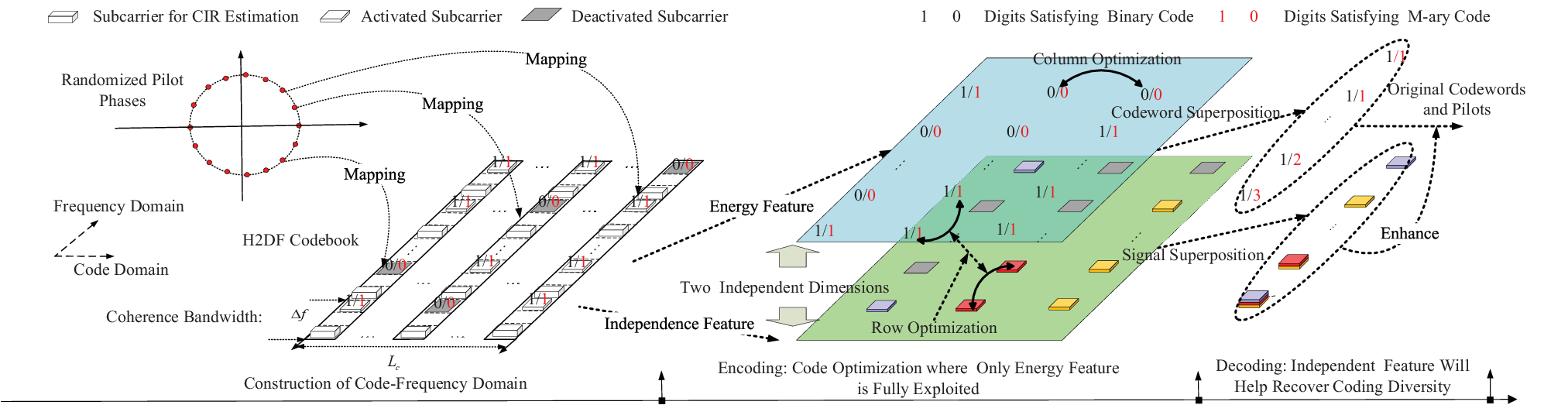
The above observations prompt us to establish a secure multiuser PA (SMPA) mechanism from the point of view of a pure coding approach and also a multi-user perspective. As shown in Fig. 1 (a), pilot randomization is a prerequisite. Then the procedures of pilot conveying, separation and identification [5, 7] are adopted, but with extra basic considerations.
Procedure 1 (Pilot Conveying).
Selectively activating and deactivating the OFDM subcarriers to create various subcarrier activation pattern (SAP) candidates; Encoding SAPs in such a way that those SAPs can carry pilot information in the form of codewords;
We emphasise that the pilot information in this paper refers to the pilot phases which are then randomized. More clearly and intuitively, the overall process is depicted in Fig. 1 (b) and described as follows:
We insert multiuser pilot tones into subcarriers on TFRG in such a way that every single pilot subcarrier for SAP and those for frequency-domain subcarrier (FS) channel estimation ( thus for channel impulse response(CIR) estimation) are located within the range of coherence bandwidth but at different frequency-domain positions. For the sake of simplicity, we configure one pilot subcarrier for FS channel estimation and one paired pilot subcarrier for SAPs. This operation guarantees the mutual independence of FS channels among adjacent positions of each SAP.
On this basis, each LU independently conveys their own pilot phase in the form of encoded SAPs which are programmed by codewords. The specific principle is that if the -th digit of the codeword is equal to 1, the pilot tone signal is inserted on the -th subcarrier, otherwise this subcarrier will be idle. In what follows, pilot separation and identification naturally means codeword separation and identification.
In this context, the attacks will be transformed from PTJ, PTS, PTN into the following hybrid mode:
Problem 1 (Attack Model).
A hybrid attack will include:
- 1.
Silence Cheating (SC): Ava keeps silence to misguide Alice since Alice cannot recognize the non-existence of attacks.
- 2.
Wide-Band Pilot (WB-PJ): Ava activates the whole available subcarriers and thus launches WB-PJ attack to interfere LUs. Therefore, the interpreted codeword at Alice is a vector with all elements“1”, which carries no information.
- 3.
Partial-Band Pilot Jamming (PB-PJ): Ava arbitrarily activates part of the subcarriers and launches PB-PJ attack. The codeword interpreted from the observation subcarriers at A Jamming lice is seriously interfered and misguided if no special coding measure is taken.
- 4.
Unpredictability: Ava could learn the pilot tones employed by each of LUs in advance and jamming/spoofing/nulling the pilot tones of arbitrary one LU of interest. This is done by searching the list of target LUs in store for attacking. This list is only known by Ava and unpredictable for both Alice and LUs.
Now the security goals require not only maintaining PA among LUs but also protecting those established PA from being attacked. We can see that PA is a probabilistic event and the security goal turns to be the reliability of pilot encoding/decoding.
We denote the first requirement by the Multiuser Guarantee which is demonstrated in Problem 2 and denote the second one by the Attack Resistance for which the attack model is given in Problem 1. The relationship among pilot randomization, multiuser guarantee and attack resistance is depicted in Fig. 1 (a).
Problem 2 (Multiuser Guarantee).
The multiuser guarantee that is ensured by codewords includes three aspects:
- P. 2.1
-
Unique Pre-Separation Identification (UPrSI): To guarantee that each codeword has a unique identifer.
- P. 2.2
-
Uniquely Decipherable (UD): P. 2.2.1: To guarantee that each superposition of up to different codewords is unique. P. 2.2.2: To guarantee that each of the superimposed codeword can be correctly decomposed into a unique set of codewords.
- P. 2.3
-
Unique Post-Separation Identification (UPoSI):To ensure that each of decomposed codewords is identified uniquely.
For the second procedure to be designed, we stress that multiuser guarantee and attack resistance must be considered.
Procedure 2 (Pilot Separation and Identification: A Mathematical Problem).
Those codewords for pilot conveying should be optimized such that those codewords, though overlapped with each other (Multiuser Guarantee) and/or even disturbed by Ava (Attack Resistance), can be separated and identified with high reliability, thus decoded into the original pilots.
Having understood above procedures theoretically, we now turn to generally introduce the practical procedures as the Fig. 1 (b) indicates. LUs and Ava create SAPs representing their own randomized pilot phases to be transmitted. Those SAPs, after undergoing wireless channels, suffer from the superposition interference from each other, and finally are superimposed and observed at Alice which separates and identifies those pilots. This is a basic process of multiuser PA. Finally those authenticated pilots are utilized for channel estimation using the estimator in [5]. Until now, we have clarified the procedures and key issues for achieving SMPA.
I-C Contributions
Solving above issues requires a reliable coding support. In a physical sense, the signals from each node carry a lot of features, such as, energy, independence and so forth, depending on how each node uses it. Different from the previous extra information, like spatial correlation information, these signal features, when generated, have already been hidden in the signals and thus there is no need to provide them priorly by system operators. The key is whether or not we could dig them out and how we use them.
For the first time, we propose exploiting those signal features to secure information coding and aim to answer the question, namely, can the hidden signal features improve the performance reliability of conventional coding technique in attack environment? We show the answer is yes, and stress that this novel and general comprehension towards coding technique constitutes the core of our H2DF coding theory.
Before detailing our contributions, we need to clearly understand what type of signal structures Alice can employ, and recognize the steps involved. In this paper, four basic steps are modeled, including 1. extracting features, i.e., energy feature and independence feature; 2. representing features; 3. encoding features; 4. decoding features. Of all the four steps, feature encoding and decoding are the core components determining the final performance of SMPA mechanism. Along the lines of Procedure 1 and 2, we summarize the main contributions of this paper as follows:
- 1.
Basically and inevitably, we consider examining the superposition characteristics of multiple potential signals on each single pilot subcarrier. We find that thanks to the indelible and unique nature of the signal energy from each node, we could extract and represent the energy feature through the well-known energy detection technique as the number of signals detected on each subcarrier. We encode the derived number as code digits (including binary digits) and construct a code-frequency domain on which we formulate feature encoding matrices in the form of codebooks by deliberately grouping the digits into codewords. Each binary codeword within codebooks could precisely indicates how each of SAPs is triggered, thus achieving Procedure 1.
- 2.
1) We further identify the second feature as the independence feature of pilot signals from each node. A differential coding technique is well designed to fully extract and represent this kind of feature as the binary code. In this way, the previous feature encoding matrices is enabled to include the code information of both energy and independence features. The feature encoding matrices are optimized by subtly coupling the differential code with the cover-free code with the aim of supporting multiuser guarantee, which constitutes the encoding functionality of H2DF coding theory. 2) For the decoding functionality, we construct a hierarchical decoding (HD) model to achieve attack resistance on the basis of multiuser guarantee, which finally realizing Procedure 2.
- 3.
The reliability of the overall encoding and decoding represents the resilience performance of SMPA against attacks. To characterize this metric, we formulate the concept of identification error probability (IEP), bounded by the exact upper and lower bounds. This phenomenon of bound fluctuation due to the random selection of the codewords by each node indicates the long-term instability in SMPA. In order to reduce this instability, a tradeoff between the upper and lower bounds is discovered, which prompts us to formally develop the bound contraction theory to further shrink the bound interval. A technique of codebook partition is proposed to achieve this successfully and an optimal upper-lower bound tradeoff is realized. Under this tradeoff, an exact closed-form expression of IEP is derived, thus creating a stable and highly-reliable SMPA performance.
Organization: In Section II, we present an overview of pilot-aware attack on multi-user PA in multi-antenna OFDM systems. In Section III, we introduce the encoding principle of H2DF coding theory. The decoding principle of H2DF coding theory is described in Section IV. A reliability bound contraction theory is provided in Section V. Simulation results are presented in Section VI and finally we conclude our work in Section VII.
Notations: We use boldface capital letters for matrices, boldface small letters for vectors , and small letters for scalars. , , and respectively denotes the conjugate operation, the transpose, the conjugate transpose and the first columns of matrix . denotes the Euclidean norm of a vector or a matrix. is the cardinality of a set. is the expectation operator. denotes the Kronecker product operator. stands for the diagonal matrix with the elements of column vector on its diagonal.
II Multi-User PA under Pilot Aware Attack: Issues and Challenges

We in this section outline a fundamental overview of multi-user PA issue under pilot aware attack, from a mathematical point of view. We will begin the overview by introducing the basic system and signal model, and then demonstrate this issue. Besides this, we will describe the advantage of pilot randomization in avoiding this issue and most importantly, identify the key challenge.
| Notations | Description |
| , | Number of transmitting antennas at BS and number of LUs. |
| Number of subcarriers for CIR estimation: for the -th LU; for Ava. | |
| Number of subcarriers for performing SAPs: for the -th LU; for Ava. | |
| ; | Index set of LUs; Index set of columns employed by LUs in . |
| , | Index set of subcarriers for CIR Estimation: for the -th LU; for Ava. |
| , | Index set of subcarriers for performing SAPs and coding: for the -th LU; for Ava. |
| ; | Pilot tones at the -th subcarrier and -th symbol time: for the -th LU; for Ava. |
| , ; , | Uplink training power: the -th LU; for Ava; Pilot phases: the -th LU; for Ava. |
| ; | CIR vectors, respectively from the -th LU and Ava to the -th receive antenna of Alice. |
| ; | Number of sampled multi-path taps in baseband, Average noise power of Alice. |
| ; ; | DFT matrix; ; Channel coherence time |
| , | Noise vector on time domain at the -th antenna of Alice within the -th symbol time. |
| ; | ; Set of OFDM symbols within . |
| Number of signals detected on the -th subcarrier. | |
| Receiving signals stacked at the -th subcarrier within the -th OFDM symbol. | |
| Noise signals at the -th subcarrier; | |
| ; | Channel frequency response vectors of the -th LU and that of Ava at the -th subcarrier. |
| ; | Jamming pilot symbols of Ava on the -th subcarrier; Codeword of Ava. |
| and | SP sum and ASP sum of H2DF codewords from all LUs; |
| and | SP sum and ASP sum of with H2DF codewords from all LUs; |
| ; ; ; ; | The -th () element of , , , and . |
| and | Set of all column vectors of and ; |
| Set of position indices of digits in . , . |
II-A System Description and Problem Model
We consider a synchronous multi-user multiple-input single-output (MISO)-OFDM systems with a -antenna Alice and single-antenna LUs. Here, pilot tone based multi-user channel estimation is considered in the uplink [6]. Conventionally, multi-user PA is accomplished by assigning LUs with publicly-known and deterministic pilot tones that can be identified. This mechanism is very fragile and actually has no privacy. Without imitating the identities of LUs, Ava merely with single antenna can synchronously interfere pilot tones indexed by and launches the behaviors shown in Attack Model.
II-B Signal Model
In this subsection, we formulate the receiving signal model at Alice. To begin with, we will give the concept of pilot insertion pattern (PIP) which indicates the way of inserting pilot tones across subcarriers and OFDM symbols.
Assumption 1 (Frequency-domain PIP).
We in this paper assume for low overhead consideration and theoretical analysis. Alternatively, we can superimpose onto a dedicated pilot sequence optimized under a non-security oriented scenario and utilize this new pilot for training. At this point, can be an additional phase difference for security consideration. We do not impose the phase constraint on the PIP strategies of Ava, that is, .
Let us proceed to the basic OFDM procedure. First, the pilot tones of LUs and Ava over subcarriers are respectively stacked as by vectors and . Assume that the length of cyclic prefix is larger than the maximum length of all channels. The parallel streams, i.e., , and , are modulated with inverse fast Fourier transform (IFFT).
Then the time-domain by vector , derived by Alice after removing the cyclic prefix at the -th receiving antenna, can be written as:
| (1) |
Here, is the circulant matrices of the -th LU, with the first column given by . is a circulant matrix with the first column given by and is assumed to be independent with .
Taking FFT, Alice finally derives the frequency-domain by signal vector at the -th receive antenna as
| (2) |
where .
II-C Multi-User Channel Estimation Model
We only focus on the FS estimation model under PTS attack mode. Ava impersonates the -th LU by utilizing the same pilot tone learned. In this case, there exists and . Stacking within OFDM symbol time, we can rewrite signals in Eq. (2) as:
| (3) |
where the matrix satisfies . The vector satisfies and is also a matrix with . For simplification, we exemplify the orthogonal pilots to demonstrate the influence of PTS attack. Given the orthogonal pilots with , a least square (LS) estimation of , contaminated by with a noise bias, can be given by:
| (4) |
where is the Moore-Penrose pseudoinverse. As to describing PTN attack and PTJ attack, we can refer to the mathematical interpretation in [5]. As we can see, the channel estimation is completely paralysed and unable to be predicted in advance. Note that this phenomenon also occurs even if non-orthogonal pilots are adopted. What’s more, we stress that any prior pilot design clues given to resist attack would also give information away to Ava.
II-D Pilot Randomization and Key Challenge
Pilot randomization can avoid the pilot aware attack without imposing any prior information on the pilot design. The common method is to randomly select phase candidates. Note that each of the phase candidates is defaultly mapped into a unique quantized sample, chosen from the set . Since phase information provides the security guarantee, thus without the need of huge overheads, we make the following assumptions:
Assumption 2 (Time-domain PIP).
During two adjacent OFDM symbol time, such as, , , two pilot phases and are kept with fixed phase difference, that is, . Here, and are both random but is deterministic and publicly known.
The value of affects the reliability of proposed SMPA architecture and as discussed in the Procedure 2, pilot randomization also brings the necessity of novel coding theory.
III Hierarchical 2-D Feature Coding for SMPA Architecture: Encoding Part
Basically, any coding strategy includes the encoding and decoding part. In this section, the encoding part of H2DF coding is formulated, which embraces three parts, that is, energy feature extraction, energy feature representation (for satisfying Procedure 1) and the feature encoding (only provides the multiuser guarantee of Procedure 2).
III-A Energy Feature Extraction
A commonsense is that wireless signal energy is indelible. Using the technique of eigenvalue ratio based energy detection (ERED) in [23], we hope to precisely measure the number of aggregated signals at subcarriers. The number represents the energy feature that we could extract and encode further.
Let us focus on a physical phenomenon, that is, the signal (or energy) superposition on each single subcarrier. This will contribute to our quantitative modelling for the energy feature. On one hand, if we examine the SAPs employed by each node, we could find they are random and mutually independent, leading to the occurrence and superposition of activated and deactivated subcarriers. In other words, the number of signals on each single subcarrier and their identities are completely unknown and unpredictable. On the other hand, this uncertainty extends to the case where the attacker is involved and configure arbitrary SAPs to interfere LUs. Therefore, each subcarrier may carry at most signals and at least no signal, depending on the choices of SAPs.
To capture the variations of the number of aggregated signals on arbitrary single subcarrier, a receiving signal matrix within OFDM symbols, denoted by , is created for energy detection. Given the normalized covariance matrix defined by , we define its ordered eigenvalues by and construct the test statistics by where denotes the decision threshold. The hypothesis means that there exist signals and means the opposite.
Based on , Eq. (49) in [23] provides a decision threshold function , for measuring how many antennas on one subcarrier are required to achieve a certain probability of false alarm denoted by . Therefore, we could establish a single-subcarrier encoding (SSE) principle, finally encoding the number of detected signals into binary and -ary digits.
Definition 1 (SSE).
Given fixed and , one subcarrier can be precisely encoded if, for any , there exists a positive number such that, for all , is smaller than .
We should note that is a monotone decreasing function of two independent variables, i.e., and but a monotone increasing function of . For a given probability constraint , we could always expect a lower bound satisfying . Under this equation, we could flexibly configure , and to make approach zero [23]. We also find that the value of achieving zero- is decreased with the increase of , but increased with the increase of .
Using as the detection threshold, Alice constructs new test statistics . The hypothesis means signals coexist and means the opposite. Using this, Alice can determine the number of coexisting signals on arbitrary single subcarrier. For example, two signals are recognized only when both and hold true.
III-B Energy Feature Representation
Basically, we could derive two types of code representing the energy feature. The first one is binary code and the other one is -ary code. To formulate the code, we begin by constructing the code-frequency domain.
III-B1 Code-Frequency Domain
We denote the binary digit corresponding to the -th pilot subcarrier by satisfying:
| (5) |
Naturally, the -ary digit is defined by:
| (6) |
Furthermore, we denote a binary code vector set by with where denotes the maximum length of the code. Similarly, we denote the -ary code vector set by satisfying .
Finally, a code frequency domain with hybrid binary and -ary code digits can be formulated as a set of pairs with and where is an integer representing the subcarrier index of appearance of the code. The construction process can be depicted in Fig. 3.
III-B2 Achieving Procedure 1
Grouping the code digits on code-frequency domain, we can derive two types of codes.
Definition 2.
We call a binary matrix satisfying and a -ary matrix satisfying as the feature encoding matrices. The -th column of and are respectively denoted by and with and . We call a codeword of of length and a codeword of with the same length..
Each LU could represent its energy feature using binary codeword which also indicates its corresponding SAP.
III-B3 Codeword Arithmetic Principle
Two arithmetic operations between codewords are formulated, depending on the specific code definition.
Definition 3.
The superposition (SP) sum (designated as the digit-by-digit Boolean sum) of two -dimensional binary codewords is defined by:
| (7) |
where represents the -th element of vector . We say that a binary vector covers a binary vector if the Boolean sum satisfies
Definition 4.
The algebraic superposition (ASP) sum (designated as the digit-by-digit sum) is defined by in which two -dimensional -ary codewords satisfy:
| (8) |
where denotes the -th element of vector .

III-C Feature Encoding: Coupling Independence Features with Coding Diversity
Here we aim to further optimize the feature encoding matrix. As shown in Fig. 3, this is done, 1) by creating the potential diversity of cover-free coding across the columns of binary matrix; 2) integrating the independence feature of receiving signals into its rows and coupling it with cover-free coding naturally. We begin our discussion by introducing the fundamental notion:
Definition 5.
A binary matrix is called a H2DF- code of length , size and order , if the following conditions are satisfied:
1) The arithmetic operation among codewords in obeys the SP principle.
2) Column-Wise Cover-free Coding (Column Optimization): For arbitrary two sets of columns, i.e., such that , , and , there exists a row such that and .
3) Per-Word Independence-Aided Differential Coding (Row Optimization): For any two positions, i.e., , , on the frequency domain, one within there exists:
| (9) |
where . denotes the differential code and denotes inner product operation. represents the differential encoder with decision threshold and satisfies .
Four situations could occur on the -th pilot subcarrier: 1) No signal exists, that is, ; 2) Only signals from Eva exist, that is, ; 3) Only signals from LUs exists, that is, ; 4) Both of signals from LUs and Eva exist, that is, .
To identify the principle of designing , we give the following interpretation. According to law of large numbers, the inner product between signals from two independent individuals, i.e. a LU and Ava, approaches zero [24]. On the contrary, the inner product between signals from the same node can reach a value with its amplitude equal to one. In theory, the value of can thus be configured to be a certain value, i.e., 0.5.
Remark 1.
The diversity of column-wise cover-free coding is a pure code property, independent with the characteristic of per-word independence-aided differential coding which is intrinsically a data-driven concept. We stress that the two codes coexist without affecting each other, and naturally agree with each other when the number of antennas increases.
In what follows, we will prove that the coding diversity can perfectly provide multiuser guarantee but lack the ability of resisting attack without the assistance of the row property which has to be exploited in the decoding part. Nevertheless, we stress that the coding diversity does not make no sense. The row property has been coupled with and included in the code but not yet been exploited in the encoding procedure.
Fact 1 (Achieving Multiuser Guarantee of Procedure 2).
We in this paper consider the special case where . The cover-free coding is introduced in [25, 26]. In this case, the boolean sum of any subset of codewords in does not cover any codeword that is not in the subset. For a constant-weight H2DF- code, two arbitrary SP sums, each superimposed by codewords, are identical if and only if the two codeword sets constituting the two sums are completely identical as well. This property guarantees the UD property.
We spilt the columns of H2DF- code matrix into independent clusters. The -th cluster includes columns indexed by and constitutes a so-called submatrix denoted by which is exclusively allocated to the -th LU. Since the UD property of has been satisfied, those submatrices can naturally satisfy the properties of UPrSI and UPoSI. In this way, H2DF- code can support multiuser guarantee, provided that there is no attack.
Definition 6.
A binary matrix is called a paired H2DF- code of length , size and order , if , equal to , has its codewords obeying the ASP principle
Definition 7.
We define the SP-sum matrix , which is the collection of all of the SP sums of codewords from , taken exactly at a time. Correspondingly, the ASP-sum matrix denotes the collection of all of the ASP sums of those codewords collected from , taken exactly at a time. Each column of (or ) represents a unique SP-sum (or ASP-sum) codeword.
Let us examine the ability of column property of H2DF encoding principle in resisting attack. Ava could use its intended SAPs to cause confusion on the detection of signals on any victim subcarrier. For example, we consider cover-free codewords of three LUs, that is, , , and and an codeword from Eva, that is, . After detection, Alice could derive the final superposed binary codeword equal to , which actually indicates no any useful information and imposes huge confusion on cover-free decoding. In this case, the decoding process is imprecise and multiuser guarantee is paralyzed.
IV Hierarchical 2-D Feature Coding for SMPA Architecture: Decoding Part
We in this section attempt to build up the Attack Resistance of Procedure 2 while maintaining the perfect multiuser guarantee. Basically, we aim to reach the potential, that is, On the basis of the energy feature, Alice could take advantage of the independence feature to recover the significant potential of coding diversity for securing against the hybrid attack. This is done by upgrading the decoding part of UD property through a HD model shown in Fig. 4. In this model, operation units with specific functionalities are connected and distributed among five sub-layers, including the starting layer, input layer, hidden layer, supervision layer and output layer. In what follows, we begin our discussion by the starting layer.
IV-A Starting Layer (Signal Collection Mathematical Modeling for Signal Superposition in SMPA Architecture)
Input: Multiple independent signals from nodes.
As the start of SMPA architecture, the superposition of observed signals on subcarriers at Alice brings the superposition of SAPs and thus the superposition of codewords mathematically. Two types of codeword superposition can be characterised by:
| (10) |
and

| (11) |
where and . Here, the specific value of vector , determined by the attack behaviors, is defined by:
| (12) |
However, the mathematical hints above can not obscure the fact that what Alice actually receives on subcarriers are still superimposed signals, rather than the code digits.
Output: The superimposed signals which are stored to the data units in the next layer.
IV-B Input Layer (Feature Extraction)
Input: The superimposed signals from the previous layer.
Alice aims to extract features of superimposed signals in data units, and encode them into code digits. Depending on features involved, those superimposed signals undergo two specific independent processes (See Fig. 4), that is, energy feature extraction and independence feature extraction.
IV-B1 Energy Feature Extracting by ERED
The detection units, configured in this layer, extract energy feature from superimposed signals in the form of codewords, i. e., and . This process is same with the one shown in Section III-A. and will be delivered to the digit units configured in the next layer.
IV-B2 Independence Feature Extracting by Inner Product Operation
The inner product units are configured to extract the independence feature from the superimposed signals in the form of code matrix, namely, . See details in Algorithm 1.
Definition 8.
A 2-D Differential code is defined by a matrix with its -th row denoted by .
Thanks to the feature extraction, the derived matrix has the potential of including all the information of codewords employed by LUs and/or Ava. can contribute to the decomposition of in the sense that it can facilitate the precise detection of which is then eliminated from .
Output:, , and . Those are delivered to the digit units in the next layer.
IV-C Codeword Superposition and Uncertainty Principle
It should be stressly noted that unpredictable attack behaviors and the corresponding codewords as well as random utilization of codewords of LUs could prevent Alice from acquiring the specific codewords within . The direct result is that Alice will observe that superimposed codewords coexist with the un-superimposed ones.
This prompts us to discover and formulate the concept of CSUP, a basic and deterministic rule followed by those random codewords within under various attacks. Undoubtedly, CSUP will contribute to the clear understanding of , fundamentally facilitating the decomposition of in the following layers.
In order to uncover the secret of CSUP, we need to examine the codeword superposition process in a smart, explicit and institutive way. Let us focus on a special stacked matrix .
Definition 9.
Imagine a -by- matrix composed by where and satisfy Eq. (11). The -th column of the submatrix constituted by the first row is denoted by with . The sum of elements of is defined by with . The column index of corresponds to that of , or equivalently the index of reference digits.
We cannot know the identities of codewords within exactly. In fact, we may not care the exact identities of codewords, but instead concentrate our attention on the column and row property of from the following two views:
Fact 2 (CSUP: Un-superimposed Codewords).
If holds true, or equivalently, holds true, Alice is perfectly able to deduce that the recovered codeword at the , also namely, the exposed codeword, must be un-superimposed.
Fact 3 (CSUP: Superimposed Codewords).
For any column satisfying , a total of codewords are surely superimposed together at this column. Only the superposition version of codewords is enabled to be precisely recovered (or namely exposed) and equal to .
CSUP describes the potential structures of under hybrid attacks comprehensively. Two typical examples demonstrating CSUP could be respectively depicted in Fig. 5. Keep in mind that CSUP provides a very basic background and technical support for solving the issues in remainder of subsections. It causes us to direct our attention to the exposed codewords which are however instable to appear. Therefore, we could sufficiently believe that the following process of codeword classification and identification (CI) could be seriously destabilized. This calls for more advanced and delicate mechanism to further optimize the decoding process, which will be depicted in the following layers.
IV-D Hidden Layer (Attack Identification)
Backing to the hidden layer, we stress that this layer is different from the previous layers and begins to gradually resolve the attack related issues.
Input: , , , and in the storage units.
As shown in Fig. 4, those inputs are fed to the identification units which are responsible for two tasks, that is, 1) precisely identify the current attack mode (SC, WB-PJ or PB-PJ); 2) differentiate the observed codeword in the current mode from those codewords under potential interfering modes.
IV-D1 Identification of WB-PJ Attack
CSUP tells us that the codewords under WB-PJ attack is very distinctive compared with those under other attacks. The principle can be summarized as follows:
Proposition 1.
When zero digit does not exist in the inputs of and , WB-PJ attack happens. This unique characteristic differentiates WB-PJ attack from other two attacks, i.e., SC and PB-PJ attack.
IV-D2 Identification of SC and PB-PJ Attack
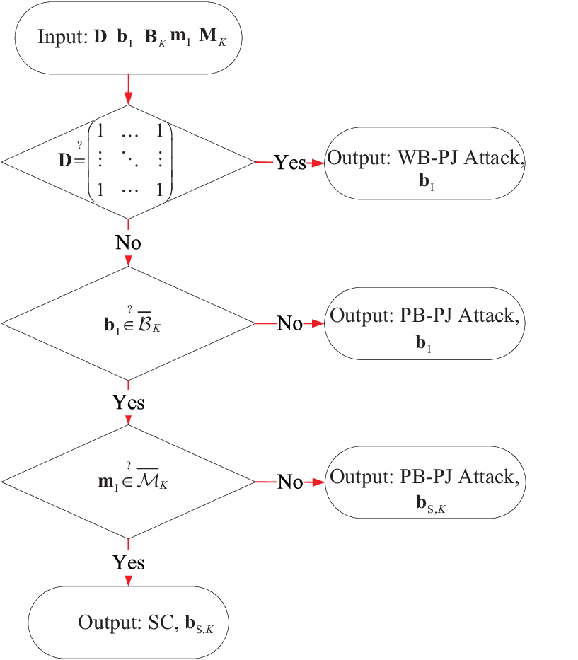
Theoretically, we need to examine the existence of and further clarify the superposition relationship between and such that we can directly identify SC and PB-PJ attack. However, what Alice observes in practice is the their superposition version, i.e., and , rather than and . We stress that and make the identification of attack more easily.
Proposition 2.
When holds true, there exists , which means that cannot be covered by . In this case, there must exist one column indexed by , such that , i.e., in , is equal to 1, with . The attack is classified as PB-PJ attack or WB-PJ attack. We can surely differentiate the PB-PJ attack from WB-PJ attack where all the inputs of are uniquely non-zero digits.
The proof is easy since if otherwise there does not exist , then must be covered by and .
Proposition 3.
When holds true, there exists and is covered by . On this basis, SC occurs if , and otherwise, PB-PJ attack happens.
In practice, we should note that the above theoretical results depend on how to determine the relationship between ( ) and (). In order to achieve this, Alice can search (), find whether or holds true and further make decisions shown in above theorems. The overall algorithm can be shown in Fig. 6.
Output: Identified attack mode and the superimposed codeword under the identified mode.
| (13) |
IV-E Supervision Layer (Codeword CI)
Input: the superimposed codeword, i.e., or , under the identified attack mode, and in the storage units.
The CI units are responsible for decomposing or , and executing the following CI task for the derived codewords.
For WB-PJ and SC attack, decomposing or could be done in Algorithm 2.
For PB-PJ attack, the flexible choices of could cause two results. 1) When , is covered by . This issue of codeword decomposition and codeword CI could be resolved using Algorithm 2. 2) Otherwise when , is not covered by . The situation is rather complicate.
In principle, the precise decomposition of into is guaranteed iff the exposed codeword (See its definition in Fact 2) is precisely identified as which is then eliminated exactly from . The challenge lies in how to identify the identities of which are usually indeterministic due to the random utilization of codewords.
Problem 3 (Indeterministic Exposed Codewords).
When PB-PJ attack happens and exists, the identities of elements in are random and unpredictable due to the random codewords employed by the overall nodes. Therefore the identities of are unknown. Any prior constraints that are imposed on the set for resolving this issue will also break down the randomness of original codewords and must not be considered.

Institutively, the precise decomposition of into is out of the question. However, if we exhaust all possibilities of which actually could be any codeword, we find that the codeword CI is intrinsically hindered by two types of confusions.
1) The identification confusion caused by when holds true. In this case, there must exist such that . Besides, we know that always holds true. Therefore, there exists the following problem:
Problem 4.
A superposition identification (SPI) problem happens, that is, cannot be differentiated from since they are both in the same matrix .
Note that the case where does not affect the ultimate decoding of codewords. Without loss of generality, we define the exact occurrence of and in by and . The identities of and are both unknown in practice. To completely resolve the above problem, we develop the technique of Back/Forward Propagation Identification (BFPI). The details are given in Algorithm 3 and an example of BFPI for 7-digit codewords under LUs can be seen in the Fig. 7.
2) The identification confusion caused by when belongs to the codebook , that is, . More specifically, could be located in any uncertain submatrix, or namely, contaminates one submatrix. There exists .
Definition 10 (Multi-User Codeword Distribution (MUCD)).
MUCD means that there always exists a unique codeword in use for each submatrix .
However, the indeterministic relationship between and exposed codeword causes a random disturbance (RD) problem in the recovery operation
Problem 5.
Confusing case: when there exist and a set such that , and are located within the same submatrix , could not be differentiated from . Identifiable case: Otherwise, could be differentiated from using Algorithm 4. This is done by examining whether or not the recovered MUCD is true. However, Alice could not predict the occurrence frequency of two cases since the exposed codewords are random, which reduces the reliability of pilot encoding/decoding in this architecture.
RD problem causes an instable codeword CI for LUs. We will analyze this phenomenon in the next section since in this section we only focus on the design of architecture.
Output: Precise under SC and WB-PJ attack; Unstably identified for PB-PJ attack,
IV-F Output Layer
This layer is configured for storing the codewords classified and identified from the previous layer.
V Reliability Bound Contraction Theory
In this section, we exploit the concept of IEP to measure the reliability of SMPA. But, our main work is to mathematically characterize the instability in this reliability and then aim to answer two questions, that is, how to reduce the instability and what level of stability can be achieved. This will be done by our proposed RBC Theory.
V-A PA Reliability and Its Instability
In this hybrid attack scenario, the codeword identification error occurs due to the PB-PJ attack, rather than WB-PJ and SC attack. This could be easily proved using Proposition 1, 2 and 3.
Theorem 1.
Given users and subcarriers, the IEP which is denoted by under H2DF- code with size is bounded by:
| (14) |
where and . The reliability of SMPA is defined by
| (15) |
Proof.
We assume that Eva is interested in the -th LU and chooses a random codeword from submatrix as . What is observed at Alice is that the exposed codewords from LUs could be randomly located in arbitrary one of possible submatrices and independent with the codeword choice of Eva. The worst case happens if the confusing case occurs. The probability is equal to and in this case, the right identification happens with probability . The final IEP is calculated as .
Otherwise, a best case (i.e., the identifiable case) occurs. The IEP is then transformed into the probability of the occurrence of duplicate codewords among the decomposed codewords , and thus calculated as . ∎
The non-tight IEP bounds tell us that the exact evaluation of SMPA reliability depends on the realization of SMPA. From a long-term perspective, we can think that the SMPA reliability fluctuates in time. Everytime SMPA is run, the differing random input (codewords) leads to a different random output, or the realization, of the SMPA process. The realization of SMPA process denoted by for the outcome IEP is the function , defined by . However, how to model the statistic process is our focus in the future and instead we hope to find a easy-to-implement technique to avoid this uncertainty smartly even though it means sacrificing some performance.
To pursue the matter further we define the maximum IEP difference between arbitrary two realizations of SMPA process within all possible time slices, as the long-term instability. More specifically, we have:
Definition 11.
The long-term instability in SMPA reliability is defined by:
| (16) |
Basically, precise repeated assessment is very critical for SMPA as we do not hope to encounter a situation where every time the system operator uses it, the evaluation of its reliability is provided imprecisely. Therefore, the proposed technique should be able to reduce to zero.
V-B Observation on the Exposed Codewords
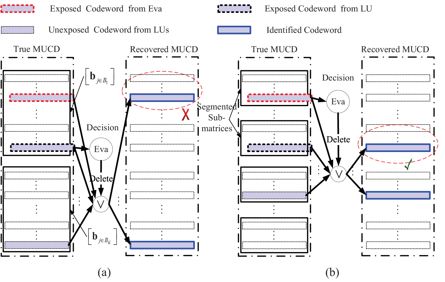
Backing to the RD problem, we find that the key of reducing lies in how to reduce the occurrence frequency of Confusing Case. Basically, it requires that Alice is able to more precisely locate the scope of the position fluctuation of exposed codewords in and further differentiate between different results. The most important is to discover the controllable variable achieving this.
We find that the submatrix-level resolution is low. We bring up the subject of the low submatrix-level resolution here as each LU is solely assigned with one submatrix and there exists only choices in total for each LU. In this sense, the low resolution makes the scope of the position fluctuation of exposed codewords relatively extensive. Therefore, everytime LUs select their own codewords obeying MUCD and Eva employs which is identical to the codeword within the same submatrix as one LU of interest, the probability that the set of exposed codewords includes is high. This can be seen in Fig. 8 (a).
However, an interesting phenomenon is that the codeword-level resolution is very high, namely, a huge number of candidate codewords for each LU exist.
V-C RBC Theory: Code Partition and Upper-Lower Bound Tradeoff
The above observation inspires us to perform codebook partition for each submatrix , in other words, the controllable variable, denoted by , now is identified as the number of segmented submatrices. Theoretically, if each of LUs is assigned with arbitrarily one of segmented submatrices, the codeword-level resolution is reduced and the lower bound of IEP is enlarged. Fortunately, the submatrix-level resolution will be thus improved and the scope of the position fluctuation of exposed codewords is restricted. Fig. 8(b) shows how the recovered MUCD in confusing case is able to be transformed to be identifiable. Then the upper bound is reduced.
Fact 4 (Upper-Lower Bound Tradeoff).
On one hand, the larger is, the lower the upper bound is. On the other hand, the larger will bring the less codewords for pilot coding and therefore the larger lower bound.
Remark 2.
Three points need to be identified. 1) Code partition does not affect the randomness of codewords; 2) Code partition does not affect the randomness of exposed codewords; 3) Code partition reduces solely the occurrence probability that both and the exposed codewords of LUs occur in one same segmented submatrix.
Note that each node does not need to inform Alice of any valuable information, such as, the index of segmented submatrix as Alice is enabled to identify the index employed because of the multiuser guarantee.
Theorem 2.
Given segmented submatrices for each submatrix, the IEP under PB-PJ attack for LUs using H2DF- code is updated and bounded by:
| (17) |
Proof.
Due to the uncertainty of which segmented submatrix is adopted by the -th LU, Eva randomly chooses a codeword in one of the segmented submatrices of as . In comparison to the worst case without code partition in Theorem 1, now the identification error happens iff there exists an exposed codeword occurring exactly within the segmented submatrix employed by Eva, rather than the original submatrix. We can calculate IEP as . For the best case, the occurrence of duplicate codewords among decomposed codewords is recalculated as since the size of codebook for pilot coding is reduced to . ∎
Theorem 3.
Given segmented submatrices for each submatrix, the optimal tradeoff between the upper and lower bounds of IEP for LUs under PB-PJ attack is achieved iff:
| (18) |
The optimal and exact expression of IEP is derived by:
| (19) |
In this case, and are respectively equal to zero and , achieving the stable and highly-reliable SMPA performance.
By configuring , we can derive the above optimal . The codeword CI can also be seen in Algorithm 4.
V-D Code Construction and Performance Analysis
In order to analyze the coding performance in practical communications systems, it is required that the expression of should be specified, which depends on the specific construction method of cover-free code. We consider the maximum distance separable (MDS) code [27] based code construction method. The reason is that such a code may be conveniently augmented with additional words, without decreasing its distance, hence its order, (or namely the number of LUs) by letting the number of ones increases suitably. It means that this method is resilient even when signals on subcarriers are interfered and thus the number of signals in detection is changed. The specific construction method can be found in [25]. The overall performance of H2DF- code here refers to the code rate, antenna and frequency-domain resource overheads and IEP.
The rate of H2DF- code of length and cardinality , denoted by , is defined in [26] by:
| (20) |
Under MDS code based code construction, the size of satisfies , which mathematically denotes the frequency-domain resource overheads. Considering the H2DF encoding process, we notice that the detection process depends on and and the codebook formulation process depends on and . Therefore, we introduce the function relationship among , and as follows:
| (21) |
where the function is the one defined by the Eq. (49) in [23].


(a) (b) (c)


(a) (b) (c)
The IEP, depending on and , thus can be formulated as follows:
Theorem 4.
With MDS based code construction method for H2DF- code, IEP can be simplified into:
| (22) |
where , .
Using , Eq. (19) and (21), we can easily derive the above theorem.
VI Simulation Results
| Simulation Parameters | Values |
| City scenario | Urban/non-line-of-sight (NLOS) |
| Antennas at BS | Uniform linear array (ULA) |
| Maximum number of LUs | |
| Channel fading and scattering model | Rayleigh and One-ring [5] |
| Carrier frequency | 2GHz |
| Bandwidth | 20MHz |
| Coherence bandwidth | 20KHz |
| Coherence time | |
| Maximum velocity of LUs | =360km/h |
| Available subcarriers for H2DF coding | ; |
| Available subcarriers for CIR estimation | ; |
| Number of channel taps | ; |
| Pilot insertion mode for CIR estimation | Block type |
| Channel estimator | [5] |
| Modulation | OFDM with normal CP |
| Slot structure | 1 slot= 7 OFDM symbols |
In this section, we simulate the performance of SMPA from two main perspectives, that is, the coding perspective and the CIR estimation perspective. For the former, we focus on five metrics, that is, the code rate, upper-lower bound tradeoff curve, the curve of instability variations, the IEP curve under the optimal bound tradeoff and the overheads in coding. We are more concerned about the configuration of system parameters, i.e., , , , , on the impact of those metrics. Usually, is set to be 2 and 3, which is enough under the practical system configuration. We should also note that is a function of and . Based on the constraint of the prime power , we know that is bounded by . Under this condition, we configure and artificially and examine the influence of variations of on the code rate. To evaluate other four metrics, we assume that always achieves its lower bound, that is, . For the channel estimation part, we consider the basic configuration shown in Table II.
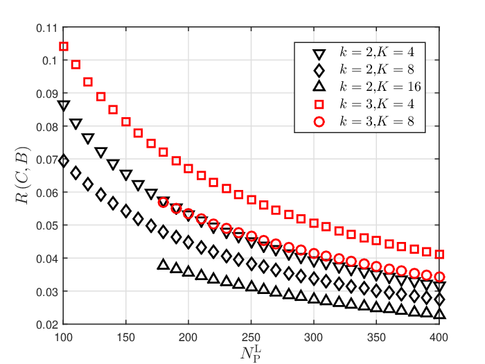
Fig. 9 (a) presents the curve of code rate versus . It indicates us three facts: 1) Increasing and will lower down the code rate; For example, the code rate ranges from 0.04 to 0.03 when increasing from 4 to 16 at and . 2) Increasing will increase the code rate; For example, the code rate increases from 0.03 to 0.04 if is increased from 2 to 3 when and .3) Increasing will increase the overheads of since the lower bound of available , that is, , increases with the increase of . For example, when , the increase of from 4 to 8 will bring the lower bound of increasing from 72 to 272.
Fig. 9(b) presents the upper-lower bound tradeoff curve. We plot ten discrete points on which there exists a relationship between the upper bound and lower bound . is configured from 1 to 10. The reason is that should be no more than the optimal value, i.e., . In this context, we configure to be 2 and 3 and to be 2 and 8. As we can see, there exists a tradeoff curve on which the upper bound has to be sacrificed to maintain a certain level of lower bound.
Fig. 9 (c) presents the curves of instability in SMPA reliability versus the number of segmented submatrices under . Considering Eq.(16) and Eq.(17), we can know that is equal to:
| (23) |
where and . From the curves, we can see that the increase of makes the instability approach zero more quickly. This demonstrates that our proposed RBC theory is very suitable for multiuser environment.
Fig. 10(a) presents the value of IEP versus . It indicates us three facts: 1) Increasing and will lower down the IEP; For example, IEP ranges from to with the increase of from 2 to 3 when and . When and , IEP decreases from to with the increase of from 250 to 400. 2) Increasing will increase the IEP; For example, when and , the IEP increases from to and further to , with the increase of from 4 to 8 to 16. 3) Increasing will also increase the overheads of since the lower bound of available increases with the increase of . In literature [7], the IEP performance is 0.5 if the two conditions hold true: 1) Eva launches randomly-imitating attack after acquiring and 2) Its array spatial fading correlation is not known by Alice, or otherwise Eva has the same mean AoA with LU of interest. In comparison to the scheme in [7], our scheme is more robust under the three conditions and able to break down this IEP floor, i.e., 0.5, because it is a pure information coding technique, not depending on the spatial fading correlation models.
In Fig. 10(b), we simulate the coding overheads in the respect of . Note that the antenna resource overheads in terms of can be seen Fig. . We do not simulate it again here. As we can see, increases linearly with the increase of the size of codebook, i.e., , or equivalently . Theoretically, is a linear function of when . For example, when changes from 12 to 20 at , namely, increases from 144 to 400, increases about from 108 to 180.
In Fig. 10(c), we stimulate the performance of CIR estimation. Normalized mean squared error (NMSE) is simulated versus signal-to-noise ratio (SNR) of LUs under arbitrary SNR of Ava. For the sake of simplicity, we assume . The performance under this type of estimator is not influenced by the specific value of due to the subspace projection property. We do not consider the case where there is no attack since in this case LS estimator is a natural choice. The CIR estimation under PTS attack is only presented since the estimation error floor under PTN and PTJ attack can be easily understood to be very high. The binned scheme proposed in [22] is simulated as an another comparison scheme. As we can see, attack could cause a high-NMSE floor on CIR estimation. This phenomenon can also be seen in the binned scheme [22]. However, the estimation in our proposed framework breaks down this floor and its NMSE gradually decreases with the increase of transmitting antennas and gradually approaches the NMSE curve under perfect minimum mean-square error (MMSE) case which serves as a performance benchmark.
VII Conclusions
In this paper, we designed a H2DF coding theory for a multi-user multi-antenna OFDM system to protect the pilot authentication process over frequency-selective fading channels. In this scheme, a framework of H2DF coding based encoding/decoding mechanism for randomized pilots through a HD model was developed, bringing about the benefits of stable and highly-reliable SMPA. Low IEP was formulated by upper and lower bounds. We verified the tradeoff relationship between the upper bound and lower bound. We developed a bound contraction theory through which an optimal upper-lower bound tradeoff can be achieved using a codebook partition technique such that the exact bound of IEP can be identified. Some necessary performance and simulations results were presented to verify the robustness of proposed scheme against pilot aware attack.
References
- [1] T. Bogale and L. B. Le, “Massive MIMO and mmWave for 5G wireless HetNet: Potentials and challenges," IEEE Veh. Technol. Mag., vol. 11, no. 1, pp. 64-75, Feb. 2016.
- [2] C. Shahriar, M. La Pan, M. Lichtman, T. C. Clancy, R. McGwier, R. Tandon, S. Sodagari, and J. H. Reed, “PHY-Layer resiliency in OFDM communications: A tutorial," IEEE Commun. Surveys Tuts., vol. 17, no. 1, pp. 292-314, Aug. 2015.
- [3] H. Rahbari, M. Krunz, and L. Lazos, “Swift jamming attack on frequency offset estimation: The Achilles�� Heel of OFDM systems," IEEE Trans. Mobile Comput., vol. 15, no. 5, pp. 1264-1278, May 2016.
- [4] M. Lichtman, R. P. Jover, M. Labib, R. Rao, V. Marojevic, and J. H. Reed, “LTE/LTE-A jamming, spoofing, and sniffing: Threat assessment and mitigation," IEEE Commun. Mag., vol. 54, no. 4, pp. 54-61, Apr. 2016
- [5] D. Xu, P. Ren, and J. A. Ritcey, “Optimal independence-checking coding for secure uplink training in large-scale MISO-OFDM systems,”�� [Online]. Available:https://arxiv.org/abs/1803.02089.
- [6] M. Ozdemir and H. Arslan, “Channel estimation for wireless OFDM systems," IEEE Commun. Surveys Tuts., vol. 9, no. 2, pp. 18-48, 2nd Quart. 2007.
- [7] D. Xu, P. Ren, J. A. Ritcey, and Y. Wang, “Code-frequency block group coding for anti-spoofing pilot authentication in multi-antenna OFDM systems," IEEE Trans. Inf. Forensics and Security, vol. 13, no. 7, pp. 1778-1793, July 2018.
- [8] W. Tu and L. Lai, “Keyless authentication and authenticated capacity,” IEEE Trans. Inf. Theory, vol. 64, no. 5, pp. 3696-3714, May 2018.
- [9] L. Lai, H. EI Gamal, and H. V. Poor, “Authentication over noisy channels,” IEEE Trans. Inf. Theory, vol. 55, no. 2, pp. 906-916, Feb. 2009.
- [10] T. C. Clancy and N.Georgen, “Security in cognitive radio networks: threats and mitigations," in Proc. 3rd Int. Conf. CrownCom., May 2008, pp. 1-8.
- [11] T. C. Clancy, “Efficient OFDM denial: Pilot jamming and pilot nulling," in Proc. IEEE Int. Conf. Commun., June 2011, pp. 1-5.
- [12] S. Sodagari and T. Clancy, “Efficient jamming attacks on MIMO channels," in Proc. IEEE Int. Conf. Commun. (ICC), June 2012, pp. 852-856.
- [13] D. Xu, P. Ren, Y. Wang, Q. Du, and L. Sun, “ICA-SBDC: A channel estimation and identification mechanism for MISO-OFDM systems under pilot spoofing attack," in Proc. IEEE Int. Conf. Commun. (ICC), May 2017, pp. 1-5.
- [14] X. Zhou, B. Maham, and A. Hjorungnes, “Pilot contamination for active eavesdropping," IEEE Trans. Wireless Commun., vol. 11, no. 3, pp. 903-907, Mar. 2012.
- [15] D. Kapetanovic, G. Zheng, K.-K. Wong, and B. Ottersten, “Detection of pilot contamination attack using random training and massive MIMO," in Proc. IEEE Int. Symp. on Personal, Indoor and Mobile Radio Commun. (PIMRC’13), Sep. 2013, pp. 13-18.
- [16] Q. Xiong, Y.-C. Liang, K. H. Li and Y. Gong, “An energy-ratio-based approach for detecting pilot spoofing attack in multiple-antenna systems,” IEEE Trans. Inf. Forensics and Security, vol. 10, no. 5, pp. 932-940, May 2015.
- [17] Y. Wu, R. Schober, D. W. K. Ng, C. Xiao, and G. Caire, “Secure massive MIMO transmission with an active eavesdropper,” IEEE Trans. Inf. Theory, vol. 62, no. 7, pp. 3880-3900, Jul. 2016.
- [18] J.K. Tugnait, “On mitigation of pilot spoofing attack,” in Proc. 2017 IEEE Int. Conf. Acous. Speech Signal Proc., Mar. 2017, pp. 2097-2101.
- [19] D. Kapetanovic, A. Al-Nahari, A. Stojanovic, and F. Rusek, “Detection of active eavesdroppers in massive MIMO,” in Proc. IEEE Int. Symp. on Personal Indoor and Mobile Radio Commun. (PIMRC’14), Sep. 2014, pp. 585-589.
- [20] J. M. Kang, C. In, and H. M. Kim, “Detection of pilot contamination attack for multi-antenna based secrecy systems,” in Proc. IEEE Vehicular Technology Conf. (VTC Spring), May 2015, pp. 1-5.
- [21] A. Adhikary, J. Nam, J.-Y. Ahn, and G. Caire, “Joint spatial division and multiplexing-The large-scale array regime,,” IEEE Trans. Inf. Theory, vol. 59, no. 10, pp. 6441-6463, Oct. 2013.
- [22] C. Shahriar and T. C. Clancy, “Performance impact of pilot tone randomization to mitigate OFDM jamming attacks," in Proc. IEEE CCNC, Jan. 2013, pp. 813-816.
- [23] H. Kobeissi, A. Nafkha, Y. Nasser, O. Bazzi, and Y. Lout, “Simple and accurate closed-form approximation of the standard condition number distribution with application in spectrum sensing,” in Proc. International Conference on Cognitive Radio Oriented Wireless Networks, May, 2016, pp. 351-362.
- [24] Z. D. Bai and J. W. Silverstein, Spectral Analysis of Large Dimensional Random Matrices, 2nd ed. Springer Series in Statistics, New York, NY, USA, 2009.
- [25] W. H. Kautz and R. C. Singleton, “Nonrandom binary superimposed codes,” IEEE Trans. Inf. Theory, vol. 10, no. 4, pp. 363-377, Oct. 1964.
- [26] A. G. D’yachkov, V. S. Lebedev, P. A. Vilenkin, and S. M. Yekhanin, “Cover-free families and superimposed codes: constructions, bounds, and applications to cryptography and group testing,” in Proc. 2001 IEEE International Symposium on Information Theory, June, 2001, pp. 117-117.
- [27] R. C. Singleton, “Maximum distance q-nary codes” IEEE Trans. Inf. Theory, vol. 10, no. 2, pp. 116-118, Apr. 1964.