跳到论文正文
W Papers独立论文阅读器 arXiv:1901.06341 论文正文 计算阅读时间 · 0%
引用这篇论文根据当前论文元数据生成,正式投稿前建议核对。


License: arXiv.org perpetual non-exclusive license
arXiv:1901.06341v1 [cs.IT] 18 Jan 2019

On Distance Properties of Convolutional Polar Codes

Ruslan Morozov       Peter Trifonov    Thanks: The authors are with the Saint Petersburg Polytechnic University, Russia. E-mail: {rmorozov, petert}@dcn.icc.spbstu.ru
Abstract

A lower bound on minimum distance of convolutional polar codes is provided. The bound is obtained from the minimum weight of generalized cosets of the codes generated by bottom rows of the polarizing matrix. Moreover, a construction of convolutional polar subcodes is proposed, which provides improved performance under successive cancellation list decoding. For sufficiently large list size, the decoding complexity of convolutional polar subcodes appears to be lower compared to Arikan polar subcodes with the same performance. The error probability of successive cancellation list decoding of convolutional polar subcodes is lower than that of Arikan polar subcodes with the same list size.

Index Terms: 
Convolutional polar codes, polar codes, successive cancellation decoding, list decoding, polar subcodes.

I Introduction

In this paper we consider codes that were firstly introduced as branching-MERA codes [1] and then as convolutional polar codes (CvPCs) [2] by A. J. Ferris, C. Hirche and D. Poulin. These codes were shown to provide substantially better performance under successive cancellation (SC) decoding compared to classical polar codes [3]. In [2] both open-boundary and periodic-boundary CvPCs are presented, in this paper by CvPCs we always mean open-boundary CvPCs. In [4] the efficient min-sum implementation of SC decoding is presented for CvPCs, which requires one to perform only comparisons and additions and can be easily extended to the case of SC list (SCL) decoding. Other implementations of SCL decoding for CvPCs are presented in [5, 6].

Classical polar codes provide quite poor performance under SCL decoding due to very low minimum distance, which scales as O⁡(n)O(\sqrt{n}) [7]. Although the minimum distance of a polar code can be found simply, the problem of computing minimum distance of an arbitrary linear code is NP-complete. However, for moderate-length codes minimum distance can be obtained by method presented in [8].

The generator matrix of a CvPC consists of rows of n×nn\times n non-singular matrix Q(n)Q^{(n)}, called convolutional polarizing transformation (CvPT). In this paper we derive a tight lower bound on the minimum distance of CvPCs, based on computing the minimum weight of a coset, given by the ii-th row of CvPT, of a linear code, generated by the last n−i−1n-i-1 rows of CvPT. The weight enumerator polynomial of such coset can be expressed as Ai​(x)−Ai+1​(x)A_{i}(x)-A_{i+1}(x), where Ai​(x)A_{i}(x) is a weight spectrum of code generated by the last n−in-i rows of matrix Q(n)Q^{(n)}. In the case of polar codes, an efficient method for approximate enumerator evaluation is available [9]. However, for convolutional polar codes there are no methods for evaluation of coset enumerator.

The minimum distance of CvPCs appears to be of the same order as in the case of classical polar codes. However, by generalizing the construction of randomized polar subcodes [10] to the case of CvPC, we obtain convolutional polar subcodes (CvPSs) with reduced error coefficient, which provide superior performance under SCL decoding, compared to polar subcodes.

The paper is organized as follows. In Section II we introduce representation of linear block codes, which is natural for the cases of Arikan and convolutional polar codes. The concepts of generalized cosets and recoverable vectors are introduced in Section III and are used to obtain a lower bound on the minimum distance of linear block codes. An efficient algorithm for computing the lower bound in the case of CvPC is provided in Section IV. This algorithm is aimed to explore some properties of low-weight codewords of CvPC. These properties are used for a construction of convolutional polar subcodes, which is proposed in Section V. The performance of the proposed code construction is presented in Section VI.

II Background

II-A Notations

The following notations are used throughout the paper. 𝔽\mathbb{F} denotes the Galois field of two elements. For integer nn we denote [n]={0,1,…​n−1}[n]=\{0,1,\ldots n-1\}. For vector aa symbol abc=(ab,ab+1,…,ac)a_{b}^{c}=(a_{b},a_{b+1},\ldots,a_{c}). For two vectors aa and bb we denote their concatenation by (a,b)(a,b). For m×nm\times\ n matrix AA and sets 𝒳⊆[m]\mathcal{X}\subseteq[m], 𝒴⊆[n],\mathcal{Y}\subseteq[n], by A𝒳,𝒴A_{\mathcal{X},\mathcal{Y}} we denote the submatrix of AA with rows with indices from set 𝒳\mathcal{X} and columns with indices from set 𝒴\mathcal{Y}, indexing of rows and columns starts with zero. Similar notations are applied to vectors as well. If 𝒳=∗\mathcal{X}=* or 𝒴=∗\mathcal{Y}=*, this means that all rows or all columns of the original matrix are in the submatrix. Furthermore, A𝒳¯,𝒴¯A_{\overline{\mathcal{X}},\overline{\mathcal{Y}}} denotes submatrix of AA consisting of rows and columns with indices that are not in 𝒳\mathcal{X} and 𝒴\mathcal{Y}, respectively. The vector of ii zeroes is denoted by 𝟎i\mathbf{0}^{i}, or just by 𝟎\mathbf{0} if ii is clear from the context.

II-B A Representation of a Linear Block Code and Successive Cancellation Decoding

Consider binary linear block code in the form

{u0n−1G(n)|uℐ∈𝔽k,uℱ=𝟎},ℐ⊆[n],|ℐ|=k,\displaystyle\left\{u_{0}^{n-1}G^{(n)}\big|u_{\mathcal{I}}\in\mathbb{F}^{k},u_{\mathcal{F}}=\mathbf{0}\right\},\mathcal{I}\subseteq[n],|\mathcal{I}|=k, (1)

where G(n)G^{(n)} is an n×nn\times n non-singular binary matrix, ℐ\mathcal{I} is called information set and ℱ=[n]∖ℐ\mathcal{F}=[n]\setminus\mathcal{I} is called frozen set. The generator matrix of such code is Gℐ,∗(n)G^{(n)}_{\mathcal{I},*}. Note that any (n,k)(n,k) linear code with generator matrix GG can be expressed as in (1) with G(n)G^{(n)}, such that G=Gℐ,∗(n)G=G^{(n)}_{\mathcal{I},*} for some ℐ⊆[n]\mathcal{I}\subseteq[n]. For example, classical polar codes [3] have G(n)=F⊗mG^{(n)}=F^{\otimes m} for n=2mn=2^{m}.

For such code representation, the successive cancellation (SC) decoding method can be defined. Consider transmission of codeword c0n−1=u0n−1​G(n)c_{0}^{n-1}=u_{0}^{n-1}G^{(n)} through binary-input memoryless channel 𝒲:𝔽→𝒴\mathcal{W}:\mathbb{F}\to\mathcal{Y}. Let y0n−1y_{0}^{n-1} be the output of this channel. After demodulation, the probabilities W⁡(ci|yi)=𝒲⁡(yi|ci)/(𝒲⁡(yi|0)+𝒲⁡(yi|1))W(c_{i}|y_{i})=\mathcal{W}(y_{i}|c_{i})/\left(\mathcal{W}(y_{i}|0)+\mathcal{W}(y_{i}|1)\right) for ci∈𝔽c_{i}\in\mathbb{F} are provided to the decoding algorithm. Given the prior hard decisions u^0​…​u^φ−1\hat{u}_{0}\ldots\hat{u}_{\varphi-1}, at phase φ\varphi the SC decoding algorithm calculates probabilities Wn(φ)​(u^0φ−1,uφ|y0n−1)W^{(\varphi)}_{n}(\hat{u}_{0}^{\varphi-1},u_{\varphi}|y_{0}^{n-1}), defined as

Wn(φ)​(u0φ|y0n−1)=∑uφ+1n−1∈𝔽n−φ−1Wn​(u0n−1​G(n)|y0n−1),\displaystyle W^{(\varphi)}_{n}(u_{0}^{\varphi}|y_{0}^{n-1})=\sum_{u_{\varphi+1}^{n-1}\in\mathbb{F}^{n-\varphi-1}}W^{n}(u_{0}^{n-1}G^{(n)}|y_{0}^{n-1}), (2)

where Wn​(c0n−1|y0n−1)=∏i=0n−1W⁡(ci|yi)W^{n}(c_{0}^{n-1}|y_{0}^{n-1})=\prod_{i=0}^{n-1}W(c_{i}|y_{i}). The channels Wn(φ):𝒴→𝔽φ+1W^{(\varphi)}_{n}:\mathcal{Y}\to\mathbb{F}^{\varphi+1} are called bit subchannels. Then, the hard decision on uφu_{\varphi} is made by

u^φ={0,φ∈ℱarg⁡maxuφ∈𝔽​Wn(φ)​(u^0φ−1,uφ|y0n−1),φ∉ℱ.\displaystyle\hat{u}_{\varphi}=\begin{cases}0,&\varphi\in\mathcal{F}\\ \arg\displaystyle\max_{u_{\varphi}\in\mathbb{F}}W^{(\varphi)}_{n}(\hat{u}_{0}^{\varphi-1},u_{\varphi}|y_{0}^{n-1}),&\varphi\notin\mathcal{F}.\end{cases}

The SC decoding can be defined for any linear code, if an efficient method for computing Wn(φ)​(u0φ|y0n−1)W^{(\varphi)}_{n}(u_{0}^{\varphi}|y_{0}^{n-1}) is available. However, SC decoding can provide reasonable performance only for codes with G(n)G^{(n)}, such that the capacities of bit subchannels Wn(φ)W^{(\varphi)}_{n} polarize, i.e. converge to 00 or 11 with n→∞n\to\infty.

II-C Convolutional Polar Codes

Convolutional polar codes [2] (CvPCs) are a family of linear block codes, for which G(n)G^{(n)}, n=2mn=2^{m}, is equal to the matrix of convolutional polarizing transformation (CvPT) Q(n)Q^{(n)}, such that

Q(n)=(X(n)​Q(n/2),Z(n)​Q(n/2)),\displaystyle Q^{(n)}=\left(X^{(n)}Q^{(n/2)},Z^{(n)}Q^{(n/2)}\right), (3)

where Q(1)=(1)Q^{(1)}=(1), X(l)X^{(l)} and Z(l)Z^{(l)} are l×l/2l\times l/2 matrices, defined for even ll as

Xi,j(l)={1,if ​2​j≤i≤2​j+20,otherwise\displaystyle X^{(l)}_{i,j}=\begin{cases}1,&\text{if }2j\leq i\leq 2j+2\\ 0,&\text{otherwise}\end{cases} (4)
Zi,j(l)={1,if ​2​j<i≤2​j+20,otherwise\displaystyle Z^{(l)}_{i,j}=\begin{cases}1,&\text{if }2j<i\leq 2j+2\\ 0,&\text{otherwise}\end{cases} (5)

For example, X(4)=(11100011)TX^{(4)}=\begin{pmatrix}1110\\ 0011\end{pmatrix}^{T}, Z(4)=(01100001)TZ^{(4)}=\begin{pmatrix}0110\\ 0001\end{pmatrix}^{T}. Expansion (3) corresponds to one layer of CvPT. In Fig. 1, the mm-th layer of CvPT is a mapping of vector u0n−1u_{0}^{n-1} to vectors x0n/2−1=u0n−1​X(n)x_{0}^{n/2-1}=u_{0}^{n-1}X^{(n)} and z0n/2−1=u0n−1​Z(n)z_{0}^{n/2-1}=u_{0}^{n-1}Z^{(n)}.

……………u0u_{0}u1u_{1}u2u_{2}u3u_{3}x0x_{0}z0z_{0}x1x_{1}z1z_{1}un−1u_{n-1}un−2u_{n-2}un−3u_{n-3}un−4u_{n-4}zn2−1z_{\frac{n}{2}-1}xn2−1x_{\frac{n}{2}-1}zn2−2z_{\frac{n}{2}-2}xn2−2x_{\frac{n}{2}-2}zn2−1z_{\frac{n}{2}-1}z1z_{1}z0z_{0}xn2−1x_{\frac{n}{2}-1}x1x_{1}x0x_{0}Q(n/2)Q^{(n/2)}Q(n/2)Q^{(n/2)}cn−1c_{n-1}cn2+1c_{\frac{n}{2}+1}cn2c_{\frac{n}{2}}cn2−1c_{\frac{n}{2}-1}c1c_{1}c0c_{0}
Fig. 1: Convolutional polarizing transformation Q(n)Q^{(n)}.

It is shown in [4] that for n=2mn=2^{m}, φ∈[n]\varphi\in[n], the value of Wn(φ)​(u0φ|y0n−1)W^{(\varphi)}_{n}(u_{0}^{\varphi}|y_{0}^{n-1}) for CvPT can be recursively computed as

Wn(2​ψ)​(u02​ψ|y)=∑wWn/2(ψ)​((u02​ψ,w)​X(2​ψ+2)|y′)\displaystyle W^{(2\psi)}_{n}(u_{0}^{2\psi}|y)=\sum_{w}W^{(\psi)}_{n/2}\left((u_{0}^{2\psi},w)X^{(2\psi+2)}\big|y^{\prime}\right)
×Wn/2(ψ)​((u02​ψ,w)​Z(2​ψ+2)|y′′)\displaystyle\times W^{(\psi)}_{n/2}\left((u_{0}^{2\psi},w)Z^{(2\psi+2)}|y^{\prime\prime}\right) (6)
Wn(2​ψ+1)​(u02​ψ+1|y)=∑u2​ψ+2,wWn/2(ψ+1)​((u02​ψ+2,w)​X(2​ψ+4)|y′)\displaystyle W^{(2\psi+1)}_{n}(u_{0}^{2\psi+1}|y)=\!\!\!\sum_{u_{2\psi+2},w}\!\!W^{(\psi+1)}_{n/2}\!\!\left((u_{0}^{2\psi+2},w)X^{(2\psi+4)}\big|y^{\prime}\right)
×Wn/2(ψ+1)​((u02​ψ+2,w)​Z(2​ψ+4)|y′′)\displaystyle\times W^{(\psi+1)}_{n/2}\!\left((u_{0}^{2\psi+2},w)Z^{(2\psi+4)}\big|y^{\prime\prime}\right) (7)
Wn(n−1)​(u0n−1|y)=Wn/2(n/2−1)​(u0n−1​X(n)|y′)\displaystyle W^{(n-1)}_{n}(u_{0}^{n-1}|y)=W^{(n/2-1)}_{n/2}\left(u_{0}^{n-1}X^{(n)}\big|y^{\prime}\right)
×Wn/2(n/2−1)​(u0n−1​Z(n)|y′′)\displaystyle\times W^{(n/2-1)}_{n/2}\left(u_{0}^{n-1}Z^{(n)}\big|y^{\prime\prime}\right) (8)

for 0≤ψ<n/2−10\leq\psi<n/2-1, where y=y0n−1y=y_{0}^{n-1}, and y′=y0n/2−1y^{\prime}=y_{0}^{n/2-1}, y′′=yn/2n−1y^{\prime\prime}=y_{n/2}^{n-1} are subvectors of yy. These formulae are the same as in [4] under permutation of the output vector yy by the bit-reversal permutation, which is omitted from the definition (3) of CvPT for the sake of simplicity.

III A Lower Bound on The Minimum Distance of Linear Codes

III-A Basic Definitions

Let 𝕊n\mathbb{S}_{n} be the set of all linear subspaces of 𝔽n\mathbb{F}^{n}.

Denote a0l−1∙b0l−1=∑i=0l−1ai​bia_{0}^{l-1}\mathchoice{\mathbin{\vbox{\hbox{\scalebox{.5}{$\displaystyle\bullet$}}}}}{\mathbin{\vbox{\hbox{\scalebox{.5}{$\textstyle\bullet$}}}}}{\mathbin{\vbox{\hbox{\scalebox{.5}{$\scriptstyle\bullet$}}}}}{\mathbin{\vbox{\hbox{\scalebox{.5}{$\scriptscriptstyle\bullet$}}}}}b_{0}^{l-1}=\sum_{i=0}^{l-1}a_{i}b_{i}, where ai,bi∈𝔽a_{i},b_{i}\in\mathbb{F}. For vectors b(0),…,b(l−1)∈𝔽tb^{(0)},\dots,b^{(l-1)}\in\mathbb{F}^{t}, denote by ⟨b(0),…,b(l−1)⟩\langle b^{(0)},\dots,b^{(l-1)}\rangle the linear subspace of 𝔽t\mathbb{F}^{t} with basis vectors b(i)b^{(i)}, i.e.

⟨b(0),…,b(l−1)⟩={∑i=0l−1aib(i)|a0l−1∈𝔽l}.\displaystyle\left\langle{b^{(0)},\dots,b^{(l-1)}}\right\rangle=\left\{\sum_{i=0}^{l-1}a_{i}b^{(i)}\left|\right.a_{0}^{l-1}\in\mathbb{F}^{l}\right\}.

A sum over an empty set is assumed to be equal to zero, which implies ⟨⟩={𝟎t}\left\langle{}\right\rangle=\left\{\mathbf{0}^{t}\right\}, where tt is clear from the context. By abuse of notation, we write x0​x1​…​xt−1x_{0}x_{1}\dots x_{t-1} for xi∈𝔽x_{i}\in\mathbb{F} to denote a vector (x0,x1,…,xt−1)∈𝔽t(x_{0},x_{1},\dots,x_{t-1})\in\mathbb{F}^{t}.

Example 1.

It can be seen that 𝕊2={⟨⟩,⟨10⟩,⟨01⟩,⟨11⟩,⟨10,01⟩}\mathbb{S}_{2}=\left\{\left\langle{}\right\rangle,\left\langle{10}\right\rangle,\left\langle{01}\right\rangle,\left\langle{11}\right\rangle,\left\langle{10,01}\right\rangle\right\}, and |𝕊3|=16|\mathbb{S}_{3}|=16.

III-B Outline of the Approach

Consider a code 𝒫\mathcal{P} in the form (1) with ℱ=[φ]\mathcal{F}=[\varphi], i.e. the set of vectors (𝟎φ,uφn−1)​G(n)(\mathbf{0}^{\varphi},u_{\varphi}^{n-1})G^{(n)}. Code 𝒫\mathcal{P} can be split in two sets corresponding to each value of uφu_{\varphi}. Namely, 𝒫=𝒫0∪𝒫1\mathcal{P}=\mathcal{P}_{0}\cup\mathcal{P}_{1}, where 𝒫a\mathcal{P}_{a} consists of all codewords of the form (𝟎φ,a,uφ+1n−1)​G(n)(\mathbf{0}^{\varphi},a,u_{\varphi+1}^{n-1})G^{(n)}. These subsets are equal to the subsets, which probabilities are computed at the φ\varphi-th phase of the SC decoding algorithm by (2), provided that the estimated symbols u^0φ−1\hat{u}_{0}^{\varphi-1} are zero. Since we are interested in distance properties of the code, we can assume that u^0φ−1=𝟎φ\hat{u}_{0}^{\varphi-1}=\mathbf{0}^{\varphi}.

Let dn(φ)d_{n}^{(\varphi)} be the distance between 𝒫0\mathcal{P}_{0} and 𝒫1\mathcal{P}_{1}, i.e. dn(φ)=minc˙∈𝒫0,c¨∈𝒫1⁡𝐰𝐭⁡(c˙+c¨)d_{n}^{(\varphi)}=\min_{\dot{c}\in\mathcal{P}_{0},\ddot{c}\in\mathcal{P}_{1}}\mathbf{wt}(\dot{c}+\ddot{c}). Consider c˙\dot{c} and c¨\ddot{c}, for such the minimum is achieved, i.e., c˙=(𝟎φ,0,u˙φ+1n−1)​G(n)\dot{c}=(\mathbf{0}^{\varphi},0,\dot{u}_{\varphi+1}^{n-1})G^{(n)}, c¨=(𝟎φ,1,u¨φ+1n−1)​G(n)\ddot{c}=(\mathbf{0}^{\varphi},1,\ddot{u}_{\varphi+1}^{n-1})G^{(n)}, such that dn(φ)=𝐰𝐭⁡(c˙+c¨)=𝐰𝐭⁡(c~)d_{n}^{(\varphi)}=\mathbf{wt}(\dot{c}+\ddot{c})=\mathbf{wt}(\tilde{c}). Note that c~=(𝟎φ,1,u˙φ+1n−1+u¨φ+1n−1)​G(n)\tilde{c}=(\mathbf{0}^{\varphi},1,\dot{u}_{\varphi+1}^{n-1}+\ddot{u}_{\varphi+1}^{n-1})G^{(n)} corresponds to value uφ=1u_{\varphi}=1, so c~∈𝒫1\tilde{c}\in\mathcal{P}_{1}. Hence, dn(φ)d^{(\varphi)}_{n} is equal to the weight of a minimum-weight codeword from 𝒫1\mathcal{P}_{1}. In general, we can say that if u^0φ−1=u0φ−1\hat{u}_{0}^{\varphi-1}=u_{0}^{\varphi-1}, i.e., all previous symbols are estimated correctly, then the probability of erroneous estimation of uφu_{\varphi} in the case of transmission over sufficiently good binary memoryless channel is mainly defined by dn(φ)=minc∈𝒫1⁡𝐰𝐭⁡(c)d^{(\varphi)}_{n}=\min_{c\in\mathcal{P}_{1}}\mathbf{wt}(c).

In section III-C we consider the partition of 𝒫\mathcal{P} in two sets 𝒫0′\mathcal{P}^{\prime}_{0} and 𝒫1′\mathcal{P}^{\prime}_{1} not by the value of uφu_{\varphi}, but by the value of some linear combination p0j−1∙uφφ+j−1p_{0}^{j-1}\mathchoice{\mathbin{\vbox{\hbox{\scalebox{.5}{$\displaystyle\bullet$}}}}}{\mathbin{\vbox{\hbox{\scalebox{.5}{$\textstyle\bullet$}}}}}{\mathbin{\vbox{\hbox{\scalebox{.5}{$\scriptstyle\bullet$}}}}}{\mathbin{\vbox{\hbox{\scalebox{.5}{$\scriptscriptstyle\bullet$}}}}}u_{\varphi}^{\varphi+j-1} of symbols uφφ+j−1u_{\varphi}^{\varphi+j-1}. Thus, set 𝒫a′\mathcal{P}^{\prime}_{a}, a∈𝔽a\in\mathbb{F} consists of all codewords (𝟎φ,uφn−1)​G(n)(\mathbf{0}^{\varphi},u_{\varphi}^{n-1})G^{(n)} satisfying p0j−1∙uφφ+j−1=ap_{0}^{j-1}\mathchoice{\mathbin{\vbox{\hbox{\scalebox{.5}{$\displaystyle\bullet$}}}}}{\mathbin{\vbox{\hbox{\scalebox{.5}{$\textstyle\bullet$}}}}}{\mathbin{\vbox{\hbox{\scalebox{.5}{$\scriptstyle\bullet$}}}}}{\mathbin{\vbox{\hbox{\scalebox{.5}{$\scriptscriptstyle\bullet$}}}}}u_{\varphi}^{\varphi+j-1}=a.

In section III-D we consider transmission of codewords through binary erasure channel (BEC) W:𝔽→𝔽∪{ϵ}W:\mathbb{F}\to\mathbb{F}\cup\left\{\epsilon\right\}, defined as W⁡(x|x)=1−pϵW(x|x)=1-p_{\epsilon}, W⁡(ϵ|x)=pϵW(\epsilon|x)=p_{\epsilon}, where pϵp_{\epsilon} is the erasure probability. We consider mapping of the set of erased symbols ℰ⊆[n]\mathcal{E}\subseteq[n] to the set of all linear combinations of symbols uφφ+j−1u_{\varphi}^{\varphi+j-1}, which can be recovered by the receiver by given cℰ¯=(ci)i∉ℰc_{\overline{\mathcal{E}}}=(c_{i})_{i\notin\mathcal{E}}. Thus, we consider a set s⊆𝔽js\subseteq\ \mathbb{F}^{j} of all vectors p0j−1∈𝔽jp_{0}^{j-1}\in\mathbb{F}^{j}, such that the value of corresponding linear combination p0j−1∙uφφ+j−1p_{0}^{j-1}\mathchoice{\mathbin{\vbox{\hbox{\scalebox{.5}{$\displaystyle\bullet$}}}}}{\mathbin{\vbox{\hbox{\scalebox{.5}{$\textstyle\bullet$}}}}}{\mathbin{\vbox{\hbox{\scalebox{.5}{$\scriptstyle\bullet$}}}}}{\mathbin{\vbox{\hbox{\scalebox{.5}{$\scriptscriptstyle\bullet$}}}}}u_{\varphi}^{\varphi+j-1} can be recovered by receiver after erasure configuration ℰ\mathcal{E}. It appears that s∈𝕊js\in\mathbb{S}_{j}, i.e. ss is a linear subspace of 𝔽j\mathbb{F}^{j}.

In section III-E, we prove that the minimum weight of vector from 𝒫1′\mathcal{P}^{\prime}_{1} (i.e., the distance between 𝒫0′\mathcal{P}^{\prime}_{0} and 𝒫1′\mathcal{P}^{\prime}_{1}) is equal to the minimum number of erasures, such that corresponding subspace s∈𝕊js\in\mathbb{S}_{j} of coefficients of recoverable linear combinations does not include the linear combination with coefficients p0j−1p_{0}^{j-1}.

These results are combined to derive the algorithm for computing dn(φ)d_{n}^{(\varphi)} in the case of CvPC, which leads to the lower bound on minimum distance of CvPC and the construction of CvPS. Furthermore, we believe that the introduced concepts and their properties can be used for other G(n)G^{(n)} that have recursive structure.

III-C Minimum Weight of Cosets and the Minimum Distance

Definition 1.

Given an n×nn\times n non-singular matrix G(n)G^{(n)}, for a vector p∈𝔽jp\in\mathbb{F}^{j} define a generalized coset 𝒞n(φ)​(p)\mathcal{C}^{(\varphi)}_{n}(p) as

𝒞n(φ)​(p)={u0n−1​G(n)|u0φ−1=𝟎∧p∙uφφ+j−1=1},\displaystyle\mathcal{C}^{(\varphi)}_{n}(p)=\left\{u_{0}^{n-1}G^{(n)}|u_{0}^{\varphi-1}=\mathbf{0}\;\wedge\;p\mathchoice{\mathbin{\vbox{\hbox{\scalebox{.5}{$\displaystyle\bullet$}}}}}{\mathbin{\vbox{\hbox{\scalebox{.5}{$\textstyle\bullet$}}}}}{\mathbin{\vbox{\hbox{\scalebox{.5}{$\scriptstyle\bullet$}}}}}{\mathbin{\vbox{\hbox{\scalebox{.5}{$\scriptscriptstyle\bullet$}}}}}u_{\varphi}^{\varphi+j-1}=1\right\}, (9)
Remark 1.

In the case of j>n−φj>n-\varphi, we assume in (9) that ul=0u_{l}=0 for l≥nl\geq n.

We define the weight of the φ\varphi-th bit subchannel Wn(φ)W_{n}^{(\varphi)} as

dn(φ)=minc∈𝒞n(φ)​(1)⁡𝐰𝐭⁡(c).\displaystyle d^{(\varphi)}_{n}=\min_{c\in\mathcal{C}^{(\varphi)}_{n}(1)}\mathbf{wt}(c).

Observe that for all j>0j>0 one has 𝒞n(φ)​(p)=𝒞n(φ)​(p,𝟎j)\mathcal{C}^{(\varphi)}_{n}(p)=\mathcal{C}^{(\varphi)}_{n}(p,\mathbf{0}^{j}), which implies dn(φ)=minc∈𝒞n(φ)​(1,𝟎j)⁡𝐰𝐭⁡(c)d^{(\varphi)}_{n}=\displaystyle\min_{c\in\mathcal{C}^{(\varphi)}_{n}(1,\mathbf{0}^{j})}\mathbf{wt}(c).

Lemma 1.

If a linear code with minimum distance dd is generated by rows of G(n)G^{(n)} with indices from ℐ⊆[n]\mathcal{I}\subseteq[n], then

d≥minφ∈ℐ⁡dn(φ).\displaystyle d\geq\min_{\varphi\in\mathcal{I}}d^{(\varphi)}_{n}. (10)
Proof.

Consider the minimum-weight codeword c0n−1=u0n−1​G(n)c_{0}^{n-1}=u_{0}^{n-1}G^{(n)}, 𝐰𝐭⁡(c0n−1)=d\mathbf{wt}(c_{0}^{n-1})=d. Let ψ\psi be the first position of non-zero element in u0n−1u_{0}^{n-1}. Thus, ψ∈ℐ\psi\in\mathcal{I}, uψ=1u_{\psi}=1, u0ψ−1=𝟎u_{0}^{\psi-1}=\mathbf{0}, which implies c0n−1∈𝒞n(ψ)​(1)c_{0}^{n-1}\in\mathcal{C}^{(\psi)}_{n}(1) and d=𝐰𝐭⁡(c0n−1)≥dn(ψ)≥minφ∈ℐ⁡dn(φ)d=\mathbf{wt}(c_{0}^{n-1})\geq d^{(\psi)}_{n}\geq\min_{\varphi\in\mathcal{I}}d^{(\varphi)}_{n}. ∎

This bound is valid for any linear block code represented in the form of (1). However, the evaluation of dn(φ)d^{(\varphi)}_{n} is not a simple problem for an arbitrary G(n)G^{(n)}.

III-D Recoverable and erased vectors

Consider transmission of a codeword c0n−1=u0n−1​G(n)c_{0}^{n-1}=u_{0}^{n-1}G^{(n)} of a code with frozen set ℱ=[φ]\mathcal{F}=[\varphi], u0φ−1=𝟎u_{0}^{\varphi-1}=\mathbf{0} and dimension k=n−φk=n-\varphi over BEC.

The set of erased positions ℰ⊆[n]\mathcal{E}\subseteq[n] is called an erasure configuration. When erasure configuration ℰ\mathcal{E} occurs, the values cℰ¯=uφn−1​G^c_{\overline{\mathcal{E}}}=u_{\varphi}^{n-1}\hat{G} are available for the receiver, where G^=G[φ]¯,ℰ¯(n)\hat{G}=G^{(n)}_{\overline{[\varphi]},\overline{\mathcal{E}}} is k×rk\times r submatrix of G(n)G^{(n)} without rows from [φ][\varphi] and without columns from ℰ\mathcal{E}, r=n−|ℰ|r=n-|\mathcal{E}|. Denote by 𝒰\mathcal{U} the set of all u^φn−1\hat{u}_{\varphi}^{n-1} such that u^φn−1​G^=cℰ¯\hat{u}_{\varphi}^{n-1}\hat{G}=c_{\overline{\mathcal{E}}}. One can see that

𝒰={uφn−1+a0k−1|a0k−1∈cs⟂⁡(G^)},\displaystyle\mathcal{U}=\left\{u_{\varphi}^{n-1}+a_{0}^{k-1}\big|a_{0}^{k-1}\in\cs^{\perp}(\hat{G})\right\}, (11)

where for set of vectors 𝒜⊆𝔽t\mathcal{A}\subseteq\mathbb{F}^{t}, by 𝒜⟂⊆𝔽t\mathcal{A}^{\perp}\subseteq\mathbb{F}^{t} we denote the set of vectors x0t−1:∀y0t−1∈𝒜:x0t−1∙y0t−1=0x_{0}^{t-1}:\forall y_{0}^{t-1}\in\mathcal{A}:x_{0}^{t-1}\mathchoice{\mathbin{\vbox{\hbox{\scalebox{.5}{$\displaystyle\bullet$}}}}}{\mathbin{\vbox{\hbox{\scalebox{.5}{$\textstyle\bullet$}}}}}{\mathbin{\vbox{\hbox{\scalebox{.5}{$\scriptstyle\bullet$}}}}}{\mathbin{\vbox{\hbox{\scalebox{.5}{$\scriptscriptstyle\bullet$}}}}}y_{0}^{t-1}=0, and cs⁡(A)\cs(A) is the column space of matrix AA. The value uφn−1u_{\varphi}^{n-1} can be unambiguously recovered by the receiver after erasure configuration ℰ\mathcal{E} iff |𝒰|=1|\mathcal{U}|=1, i.e. 𝒰={uφn−1}\mathcal{U}=\left\{u_{\varphi}^{n-1}\right\}.

More generally, consider the recoverability of the value of a linear combination p0k−1∙uφn−1p_{0}^{k-1}\mathchoice{\mathbin{\vbox{\hbox{\scalebox{.5}{$\displaystyle\bullet$}}}}}{\mathbin{\vbox{\hbox{\scalebox{.5}{$\textstyle\bullet$}}}}}{\mathbin{\vbox{\hbox{\scalebox{.5}{$\scriptstyle\bullet$}}}}}{\mathbin{\vbox{\hbox{\scalebox{.5}{$\scriptscriptstyle\bullet$}}}}}u_{\varphi}^{n-1} after erasure configuration ℰ\mathcal{E}. The set of values of p0k−1∙u^φn−1p_{0}^{k-1}\mathchoice{\mathbin{\vbox{\hbox{\scalebox{.5}{$\displaystyle\bullet$}}}}}{\mathbin{\vbox{\hbox{\scalebox{.5}{$\textstyle\bullet$}}}}}{\mathbin{\vbox{\hbox{\scalebox{.5}{$\scriptstyle\bullet$}}}}}{\mathbin{\vbox{\hbox{\scalebox{.5}{$\scriptscriptstyle\bullet$}}}}}\hat{u}_{\varphi}^{n-1} for all u^φn−1∈𝒰\hat{u}_{\varphi}^{n-1}\in\mathcal{U} is given by

{p0k−1∙(uφn−1+a0k−1)|a0k−1∈cs⟂⁡(G^)}.\displaystyle\left\{p_{0}^{k-1}\mathchoice{\mathbin{\vbox{\hbox{\scalebox{.5}{$\displaystyle\bullet$}}}}}{\mathbin{\vbox{\hbox{\scalebox{.5}{$\textstyle\bullet$}}}}}{\mathbin{\vbox{\hbox{\scalebox{.5}{$\scriptstyle\bullet$}}}}}{\mathbin{\vbox{\hbox{\scalebox{.5}{$\scriptscriptstyle\bullet$}}}}}(u_{\varphi}^{n-1}+a_{0}^{k-1})\;\big|\;a_{0}^{k-1}\in\cs^{\perp}(\hat{G})\right\}. (12)

We say that vector p0k−1p_{0}^{k-1} is (ℰ,φ)(\mathcal{E},\varphi)-recoverable, if the corresponding linear combination p0k−1∙uφn−1p_{0}^{k-1}\mathchoice{\mathbin{\vbox{\hbox{\scalebox{.5}{$\displaystyle\bullet$}}}}}{\mathbin{\vbox{\hbox{\scalebox{.5}{$\textstyle\bullet$}}}}}{\mathbin{\vbox{\hbox{\scalebox{.5}{$\scriptstyle\bullet$}}}}}{\mathbin{\vbox{\hbox{\scalebox{.5}{$\scriptscriptstyle\bullet$}}}}}u_{\varphi}^{n-1} can be recovered unambiguously for given cℰ¯c_{\overline{\mathcal{E}}}, i.e., the set (12) contains only the correct value p0k−1∙uφn−1p_{0}^{k-1}\mathchoice{\mathbin{\vbox{\hbox{\scalebox{.5}{$\displaystyle\bullet$}}}}}{\mathbin{\vbox{\hbox{\scalebox{.5}{$\textstyle\bullet$}}}}}{\mathbin{\vbox{\hbox{\scalebox{.5}{$\scriptstyle\bullet$}}}}}{\mathbin{\vbox{\hbox{\scalebox{.5}{$\scriptscriptstyle\bullet$}}}}}u_{\varphi}^{n-1}. Expanding the brackets in (12), one can see that p0k−1p_{0}^{k-1} is (ℰ,φ)(\mathcal{E},\varphi)-recoverable iff ∀a0k−1∈cs⟂⁡(G^):p0k−1∙a0k−1=0\forall a_{0}^{k-1}\in\cs^{\perp}(\hat{G}):p_{0}^{k-1}\mathchoice{\mathbin{\vbox{\hbox{\scalebox{.5}{$\displaystyle\bullet$}}}}}{\mathbin{\vbox{\hbox{\scalebox{.5}{$\textstyle\bullet$}}}}}{\mathbin{\vbox{\hbox{\scalebox{.5}{$\scriptstyle\bullet$}}}}}{\mathbin{\vbox{\hbox{\scalebox{.5}{$\scriptscriptstyle\bullet$}}}}}a_{0}^{k-1}=0, which leads to p0k−1∈cs⟂⟂⁡(G^)=cs⁡(G^)p_{0}^{k-1}\in{\cs^{\perp}}^{\perp}(\hat{G})=\cs(\hat{G}). Thus, the set of (ℰ,φ)(\mathcal{E},\varphi)-recoverable vectors is a linear space, which is equal to cs⁡(G^)∈𝕊k\cs(\hat{G})\in\mathbb{S}_{k}.

Definition 2.

Let s∈𝕊js\in\mathbb{S}_{j} be the space of all p0j−1p_{0}^{j-1}, such that (p0j−1,𝟎k−j)(p_{0}^{j-1},\mathbf{0}^{k-j}) is (ℰ,φ)(\mathcal{E},\varphi)-recoverable. In this case, ss is called a (ℰ,φ,j)(\mathcal{E},\varphi,j)-space and is denoted by χn(φ,j)​(ℰ)\chi^{(\varphi,j)}_{n}(\mathcal{E}), and ℰ\mathcal{E} is called an (s,φ,j)(s,\varphi,j)-configuration. The set of (s,φ,j)(s,\varphi,j)-configurations is denoted by ξn(φ,j)​(s)\xi^{(\varphi,j)}_{n}(s). Thus,

χn(φ,j)​(ℰ)\displaystyle\chi^{(\varphi,j)}_{n}(\mathcal{E}) ={p0j−1|(p0j−1,𝟎k−j)∈cs⁡(G[φ]¯,ℰ¯(n))},\displaystyle=\left\{p_{0}^{j-1}\;\big|\;(p_{0}^{j-1},\mathbf{0}^{k-j})\in\cs\left(G^{(n)}_{\overline{[\varphi]},\overline{\mathcal{E}}}\right)\right\}, (13)
ξn(φ,j)​(s)\displaystyle\xi^{(\varphi,j)}_{n}(s) ={ℰ|χn(φ,j)​(ℰ)=s}.\displaystyle=\left\{\mathcal{E}\;\big|\;\chi^{(\varphi,j)}_{n}(\mathcal{E})=s\right\}. (14)

If 𝒜\mathcal{A} is a set, denote by 2𝒜2^{\mathcal{A}} the set of all subsets of 𝒜\mathcal{A}. Thus, function χn(φ,j):2[n]→𝕊j\chi_{n}^{(\varphi,j)}:2^{[n]}\to\mathbb{S}_{j}, maps an erasure configuration, which is a subset of [n][n], to a linear subspace of 𝔽j\mathbb{F}^{j}, and ξn(φ,j)\xi^{(\varphi,j)}_{n} returns the inverse image of χn(φ,j)\chi_{n}^{(\varphi,j)}. Note that χn(φ,j)\chi_{n}^{(\varphi,j)} is not injective, so ξn(φ,j):𝕊j→22[n]\xi^{(\varphi,j)}_{n}:\mathbb{S}_{j}\to 2^{2^{[n]}}.

In words, χn(φ,j)​(ℰ)\chi_{n}^{(\varphi,j)}(\mathcal{E}) defines the set of vectors p0j−1p_{0}^{j-1}, for which the value of linear combination p0j−1∙uφφ+j−1p_{0}^{j-1}\mathchoice{\mathbin{\vbox{\hbox{\scalebox{.5}{$\displaystyle\bullet$}}}}}{\mathbin{\vbox{\hbox{\scalebox{.5}{$\textstyle\bullet$}}}}}{\mathbin{\vbox{\hbox{\scalebox{.5}{$\scriptstyle\bullet$}}}}}{\mathbin{\vbox{\hbox{\scalebox{.5}{$\scriptscriptstyle\bullet$}}}}}u_{\varphi}^{\varphi+j-1} can be recovered after erasure configuration ℰ\mathcal{E}, provided that u0φ−1=𝟎u_{0}^{\varphi-1}=\mathbf{0}. Conversely, ξn(φ,j)​(s)\xi^{(\varphi,j)}_{n}(s) defines the set of erasure configurations, after which the linear combination p0j−1∙uφφ+j−1p_{0}^{j-1}\mathchoice{\mathbin{\vbox{\hbox{\scalebox{.5}{$\displaystyle\bullet$}}}}}{\mathbin{\vbox{\hbox{\scalebox{.5}{$\textstyle\bullet$}}}}}{\mathbin{\vbox{\hbox{\scalebox{.5}{$\scriptstyle\bullet$}}}}}{\mathbin{\vbox{\hbox{\scalebox{.5}{$\scriptscriptstyle\bullet$}}}}}u_{\varphi}^{\varphi+j-1} can be deduced by the receiver if and only if p∈sp\in s.

Remark 2.

Let j>kj>k, i.e. j=k+hj=k+h for some h>0h>0. In this case, the conditional part of definition (13) is inconsistent. We extend the definition as follows. In Remark 1 we assume that symbols un+hu_{n+h} for h≥0h\geq 0 are equal to zero. Hence, these symbols are always perfectly known for the receiver, so any ℰ\mathcal{E} does not erase any symbol un+hu_{n+h}. Observe that any vector from 𝔽j∖χn(φ,j)​(ℰ)\mathbb{F}^{j}\setminus\chi^{(\varphi,j)}_{n}(\mathcal{E}) must be not (ℰ,φ)(\mathcal{E},\varphi)-recoverable, so for any ℰ\mathcal{E} and q0h−1∈𝔽hq_{0}^{h-1}\in\mathbb{F}^{h}, we must include vector (𝟎k,q0h−1)(\mathbf{0}^{k},q_{0}^{h-1}) in the set χn(φ,k+h)​(ℰ)\chi^{(\varphi,k+h)}_{n}(\mathcal{E}). This leads to

χn(φ,k+h)(ℰ)={(p,q)|p∈χn(φ,k)(ℰ),q∈𝔽h}.\displaystyle\chi_{n}^{(\varphi,k+h)}(\mathcal{E})=\left\{(p,q)\;\big|\;p\in\chi_{n}^{(\varphi,k)}(\mathcal{E}),q\in\mathbb{F}^{h}\right\}.

Similarly, we assume that ξn(φ,k+h)​(s)=∅\xi^{(\varphi,k+h)}_{n}(s)=\emptyset for all ss which do not contain (𝟎k,q)(\mathbf{0}^{k},q) for some q∈𝔽hq\in\mathbb{F}^{h}.

Example 2.

Consider (s,0,2)(s,0,2)-configurations for the case of n=2n=2, c01=u01​Q(2)=(u0+u1,u1)c_{0}^{1}=u_{0}^{1}Q^{(2)}=(u_{0}+u_{1},u_{1}). For erasure configuration ℰ={0}\mathcal{E}=\{0\}, the only non-zero vector which is (ℰ,0)(\mathcal{E},0)-recoverable is p=(0,1)p=(0,1). That is, if symbol c0c_{0} is erased, one can recover unambiguously only u1=c1u_{1}=c_{1}. This means that {0}∈ξ2(0,2)​(⟨01⟩)\{0\}\in\xi^{(0,2)}_{2}(\left\langle{01}\right\rangle). All (s,0,2)(s,0,2)-configurations are

ξ2(0,2)​(⟨01⟩)={{0}},ξ2(0,2)​(⟨10⟩)=∅,ξ2(0,2)​(⟨11⟩)={{1}},\displaystyle\xi^{(0,2)}_{2}(\left\langle{01}\right\rangle)=\{\{0\}\},\xi^{(0,2)}_{2}(\left\langle{10}\right\rangle)=\emptyset,\xi^{(0,2)}_{2}(\left\langle{11}\right\rangle)=\left\{\left\{1\right\}\right\},
ξ2(0,2)​(⟨⟩)={{0,1}},ξ2(0,2)​(𝔽2)={∅}.\displaystyle\xi^{(0,2)}_{2}(\left\langle{}\right\rangle)=\left\{\left\{0,1\right\}\right\},\xi^{(0,2)}_{2}(\mathbb{F}^{2})=\{\emptyset\}. (15)

That is, there are no erasure configurations, such that only ⟨10⟩\langle 10\rangle (i.e. symbol u0u_{0}) is unambiguously recoverable, and the whole vector u01u_{0}^{1} can be unambiguously recovered only if there are no erasures. For the same case, the (ℰ,0,2)(\mathcal{E},0,2)-spaces are

χ2(0,2)​(∅)=𝔽2,χ2(0,2)​({0})=⟨01⟩,\displaystyle\chi_{2}^{(0,2)}(\emptyset)=\mathbb{F}^{2},\chi_{2}^{(0,2)}(\left\{0\right\})=\left\langle{01}\right\rangle,
χ2(0,2)​({1})=⟨11⟩,χ2(0,2)​({0,1})=⟨⟩.\displaystyle\chi_{2}^{(0,2)}(\left\{1\right\})=\left\langle{11}\right\rangle,\chi_{2}^{(0,2)}(\left\{0,1\right\})=\left\langle{}\right\rangle.
Example 3.

Consider the case of φ=2\varphi=2, j=2j=2, n=4n=4 and c03=u03​Q(4)=(u0+u1+u3,u2+u3,u1+u2+u3,u3)c_{0}^{3}=u_{0}^{3}Q^{(4)}=(u_{0}+u_{1}+u_{3},u_{2}+u_{3},u_{1}+u_{2}+u_{3},u_{3}). Since φ=2\varphi=2 implies u01=𝟎u_{0}^{1}=\mathbf{0}, one has c0=c3=u3c_{0}=c_{3}=u_{3}, c1=c2=u2+u3c_{1}=c_{2}=u_{2}+u_{3} and one can restore u3u_{3} by c0c_{0} or c3c_{3}. Thus, ξ4(2,2)​(⟨01⟩)={{1,2},{0,1,2},{1,2,3}}\xi^{(2,2)}_{4}(\left\langle{01}\right\rangle)=\left\{\left\{1,2\right\},\left\{0,1,2\right\},\left\{1,2,3\right\}\right\}.

III-E Coset minimum weight and erasure configurations

For a subspace s∈𝕊js\in\mathbb{S}_{j}, we denote the minimal cardinality of (s,φ,j)(s,\varphi,j)-configuration as

δn(φ,j)​(s)=minℰ∈ξn(φ,j)​(s)⁡|ℰ|,\displaystyle\delta^{(\varphi,j)}_{n}(s)=\min_{\mathcal{E}\in\xi^{(\varphi,j)}_{n}(s)}|\mathcal{E}|, (16)

assuming that the minimum over the empty set is +∞+\infty.

Theorem 1.

Let φ∈[n]\varphi\in[n] and j>0j>0. For any p∈𝔽jp\in\mathbb{F}^{j},

minc∈𝒞n(φ)​(p)𝐰𝐭(c)=mins∈𝕊j:p∉sδn(φ,j)(s).\displaystyle\min_{c\in\mathcal{C}^{(\varphi)}_{n}(p)}\mathbf{wt}(c)=\min_{s\in\mathbb{S}_{j}:p\notin s}\delta^{(\varphi,j)}_{n}(s).
Proof.

Denote 𝒜={supp⁡(c)|c∈𝒞n(φ)​(p)}\mathcal{A}=\left\{\supp(c)\big|c\in\mathcal{C}^{(\varphi)}_{n}(p)\right\},

ℬ\displaystyle\mathcal{B} =⋃s∈𝕊j:p∉sξn(φ,j)(s)=⋃s∈𝕊j:p∉s{ℰ|χn(φ,j)(ℰ)=s}\displaystyle=\bigcup_{s\in\mathbb{S}_{j}:p\notin s}\xi^{(\varphi,j)}_{n}(s)=\bigcup_{s\in\mathbb{S}_{j}:p\notin s}\left\{\mathcal{E}\;|\;\chi_{n}^{(\varphi,j)}(\mathcal{E})=s\right\}
={ℰ|p∉χn(φ,j)​(ℰ)}.\displaystyle=\left\{\mathcal{E}\;|\;p\notin\chi_{n}^{(\varphi,j)}(\mathcal{E})\right\}.

Then the theorem can be reformulated as minΩ∈𝒜⁡|Ω|=minℰ∈ℬ⁡|ℰ|.\min_{\Omega\in\mathcal{A}}|\Omega|=\min_{\mathcal{E}\in\mathcal{B}}|\mathcal{E}|.

If Ω∈𝒜\Omega\in\mathcal{A}, then there exists uφn−1u_{\varphi}^{n-1}, such that p∙uφφ+j−1=1p\mathchoice{\mathbin{\vbox{\hbox{\scalebox{.5}{$\displaystyle\bullet$}}}}}{\mathbin{\vbox{\hbox{\scalebox{.5}{$\textstyle\bullet$}}}}}{\mathbin{\vbox{\hbox{\scalebox{.5}{$\scriptstyle\bullet$}}}}}{\mathbin{\vbox{\hbox{\scalebox{.5}{$\scriptscriptstyle\bullet$}}}}}u_{\varphi}^{\varphi+j-1}=1 and Ω=supp⁡(c0n−1)\Omega=\supp(c_{0}^{n-1}) for c0n−1=(𝟎φ,uφn−1)​G(n)c_{0}^{n-1}=(\mathbf{0}^{\varphi},u_{\varphi}^{n-1})G^{(n)}. In this case cΩ¯=𝟎c_{\overline{\Omega}}=\mathbf{0} and the all-zero value u^φn−1=𝟎\hat{u}_{\varphi}^{n-1}=\mathbf{0} also belongs to set (11) of possible values of uφn−1u_{\varphi}^{n-1} for the given cΩ¯c_{\overline{\Omega}}, but p∙u^φφ+j−1=0p\mathchoice{\mathbin{\vbox{\hbox{\scalebox{.5}{$\displaystyle\bullet$}}}}}{\mathbin{\vbox{\hbox{\scalebox{.5}{$\textstyle\bullet$}}}}}{\mathbin{\vbox{\hbox{\scalebox{.5}{$\scriptstyle\bullet$}}}}}{\mathbin{\vbox{\hbox{\scalebox{.5}{$\scriptscriptstyle\bullet$}}}}}\hat{u}_{\varphi}^{\varphi+j-1}=0. Thus, the value of p∙uφφ+j−1p\mathchoice{\mathbin{\vbox{\hbox{\scalebox{.5}{$\displaystyle\bullet$}}}}}{\mathbin{\vbox{\hbox{\scalebox{.5}{$\textstyle\bullet$}}}}}{\mathbin{\vbox{\hbox{\scalebox{.5}{$\scriptstyle\bullet$}}}}}{\mathbin{\vbox{\hbox{\scalebox{.5}{$\scriptscriptstyle\bullet$}}}}}u_{\varphi}^{\varphi+j-1} is not recoverable after erasure configuration Ω\Omega, which implies p∉χn(φ,j)​(Ω)⟹Ω∈ℬp\notin\chi^{(\varphi,j)}_{n}(\Omega)\implies\Omega\in\mathcal{B}. So, Ω∈𝒜⟹Ω∈ℬ\Omega\in\mathcal{A}\implies\Omega\in\mathcal{B} and minΩ∈𝒜⁡|Ω|≥minℰ∈ℬ⁡|ℰ|\displaystyle\min_{\Omega\in\mathcal{A}}|\Omega|\geq\min_{\mathcal{E}\in\mathcal{B}}|\mathcal{E}|.

If ℰ∈ℬ\mathcal{E}\in\mathcal{B}, then p∉χn(φ,j)​(ℰ)p\notin\chi^{(\varphi,j)}_{n}(\mathcal{E}), which by Definition 2 implies (p,𝟎k−j)∉cs⁡(G^)(p,\mathbf{0}^{k-j})\notin\cs(\hat{G}) and ∃a0k−1∈cs⟂⁡(G^):(p,𝟎k−j)∙a0k−1=1\exists a_{0}^{k-1}\in\cs^{\perp}(\hat{G}):(p,\mathbf{0}^{k-j})~\mathchoice{\mathbin{\vbox{\hbox{\scalebox{.5}{$\displaystyle\bullet$}}}}}{\mathbin{\vbox{\hbox{\scalebox{.5}{$\textstyle\bullet$}}}}}{\mathbin{\vbox{\hbox{\scalebox{.5}{$\scriptstyle\bullet$}}}}}{\mathbin{\vbox{\hbox{\scalebox{.5}{$\scriptscriptstyle\bullet$}}}}}~a_{0}^{k-1}=~1, which implies p∙a0j−1=1p\mathchoice{\mathbin{\vbox{\hbox{\scalebox{.5}{$\displaystyle\bullet$}}}}}{\mathbin{\vbox{\hbox{\scalebox{.5}{$\textstyle\bullet$}}}}}{\mathbin{\vbox{\hbox{\scalebox{.5}{$\scriptstyle\bullet$}}}}}{\mathbin{\vbox{\hbox{\scalebox{.5}{$\scriptscriptstyle\bullet$}}}}}a_{0}^{j-1}=1. Denote c^0n−1=(𝟎φ,a0k−1)​G(n)\hat{c}_{0}^{n-1}=(\mathbf{0}^{\varphi},a_{0}^{k-1})G^{(n)}. Since p∙a0j−1=1p\mathchoice{\mathbin{\vbox{\hbox{\scalebox{.5}{$\displaystyle\bullet$}}}}}{\mathbin{\vbox{\hbox{\scalebox{.5}{$\textstyle\bullet$}}}}}{\mathbin{\vbox{\hbox{\scalebox{.5}{$\scriptstyle\bullet$}}}}}{\mathbin{\vbox{\hbox{\scalebox{.5}{$\scriptscriptstyle\bullet$}}}}}a_{0}^{j-1}=1, by Definition 1 one has c^0n−1∈𝒞n(φ)​(p)\hat{c}_{0}^{n-1}\in\mathcal{C}^{(\varphi)}_{n}(p), and therefore supp⁡(c^)∈𝒜\supp(\hat{c})\in\mathcal{A}. On the other hand, c^ℰ¯=a0k−1​G^=𝟎\hat{c}_{\overline{\mathcal{E}}}=a_{0}^{k-1}\hat{G}=\mathbf{0}, which means supp⁡(c^)⊆ℰ\supp(\hat{c})\subseteq\mathcal{E}. So, ∀ℰ∈ℬ​∃Ω∈𝒜:Ω⊆ℰ\forall\mathcal{E}\in\mathcal{B}\;\;\exists\Omega\in\mathcal{A}:\Omega\subseteq\mathcal{E}, hence, minΩ∈𝒜⁡|Ω|≤minℰ∈ℬ⁡|ℰ|\displaystyle\min_{\Omega\in\mathcal{A}}|\Omega|\leq\min_{\mathcal{E}\in\mathcal{B}}|\mathcal{E}|. ∎

Corollary 1.

For any j>0:j>0:

dn(φ)=min{δn(φ,j)(s)|s∈𝕊j:(1,𝟎j−1)∉s}.d^{(\varphi)}_{n}=\min\left\{\delta^{(\varphi,j)}_{n}(s)\big|s\in\mathbb{S}_{j}:(1,\mathbf{0}^{j-1})\notin s\right\}.

IV Bound on Minimum Distance of Convolutional Polar Codes

The structure of the convolutional polarizing transformation Q(n)Q^{(n)}, n=2mn=2^{m}, enables one to compute easily δn(φ,j)​(s)\delta^{(\varphi,j)}_{n}(s), defined in (16), for j=3j=3. By computing values of δn(φ,3)​(s)\delta^{(\varphi,3)}_{n}(s), one can obtain values of dn(φ)d^{(\varphi)}_{n} by Corollary 1 and lower bound on minimum distance by Lemma 1.

Consider transmission of c0n−1=u0n−1​Q(n)c_{0}^{n-1}=u_{0}^{n-1}Q^{(n)}, such that u0φ−1=𝟎u_{0}^{\varphi-1}=\mathbf{0}, through BEC and let the erasure configuration be ℰ\mathcal{E}. The intuition behind recursive computing of δn(φ,3)​(s)\delta^{(\varphi,3)}_{n}(s) is as follows.

Consider the case of φ=2​ψ+1<n−1\varphi=2\psi+1<n-1. Denote x0n/2−1=u0n−1​X(n)x_{0}^{n/2-1}=u_{0}^{n-1}X^{(n)}, z0n/2−1=u0n−1​Z(n)z_{0}^{n/2-1}=u_{0}^{n-1}Z^{(n)}, ℰ′=ℰ∩[n2]\mathcal{E}^{\prime}=\mathcal{E}\cap[\frac{n}{2}], ℰ′′={i≥0|i+n2∈ℰ}\mathcal{E}^{\prime\prime}=\left\{i\geq 0|i+\frac{n}{2}\in\mathcal{E}\right\}. Recall that χn(2​ψ+1,3)​(ℰ)\chi^{(2\psi+1,3)}_{n}(\mathcal{E}) is the set of all p02p_{0}^{2}, such that the value of p02∙u2​ψ+12​ψ+3p_{0}^{2}\mathchoice{\mathbin{\vbox{\hbox{\scalebox{.5}{$\displaystyle\bullet$}}}}}{\mathbin{\vbox{\hbox{\scalebox{.5}{$\textstyle\bullet$}}}}}{\mathbin{\vbox{\hbox{\scalebox{.5}{$\scriptstyle\bullet$}}}}}{\mathbin{\vbox{\hbox{\scalebox{.5}{$\scriptscriptstyle\bullet$}}}}}u_{2\psi+1}^{2\psi+3} can be deduced from c0n−1c_{0}^{n-1} after erasure configuration ℰ\mathcal{E}. Similarly, χn/2(ψ,3)​(ℰ′)\chi^{(\psi,3)}_{n/2}(\mathcal{E}^{\prime}) and χn/2(ψ,3)​(ℰ′′)\chi_{n/2}^{(\psi,3)}(\mathcal{E}^{\prime\prime}) are the sets of q02q_{0}^{2} and r02r_{0}^{2}, s.t. q02∙xψψ+2q_{0}^{2}\mathchoice{\mathbin{\vbox{\hbox{\scalebox{.5}{$\displaystyle\bullet$}}}}}{\mathbin{\vbox{\hbox{\scalebox{.5}{$\textstyle\bullet$}}}}}{\mathbin{\vbox{\hbox{\scalebox{.5}{$\scriptstyle\bullet$}}}}}{\mathbin{\vbox{\hbox{\scalebox{.5}{$\scriptscriptstyle\bullet$}}}}}x_{\psi}^{\psi+2} and r02∙zψψ+2r_{0}^{2}\mathchoice{\mathbin{\vbox{\hbox{\scalebox{.5}{$\displaystyle\bullet$}}}}}{\mathbin{\vbox{\hbox{\scalebox{.5}{$\textstyle\bullet$}}}}}{\mathbin{\vbox{\hbox{\scalebox{.5}{$\scriptstyle\bullet$}}}}}{\mathbin{\vbox{\hbox{\scalebox{.5}{$\scriptscriptstyle\bullet$}}}}}z_{\psi}^{\psi+2} are recoverable from c0n/2−1c_{0}^{n/2-1} and cn/2n−1c_{n/2}^{n-1} after erasure configurations ℰ′\mathcal{E}^{\prime} and ℰ′′\mathcal{E}^{\prime\prime}, under assumption x0ψ−1=𝟎x_{0}^{\psi-1}=\mathbf{0} and z0ψ−1=𝟎z_{0}^{\psi-1}=\mathbf{0}, respectively. By (4)–(5) one obtains xi=u2​i+u2​i+1+u2​i+2x_{i}=u_{2i}+u_{2i+1}+u_{2i+2} and zi=u2​i+1+u2​i+2z_{i}=u_{2i+1}+u_{2i+2} for i<n2−1i<\frac{n}{2}-1, which, together with u02​ψ=𝟎u_{0}^{2\psi}=\mathbf{0}, implies x0ψ−1=z0ψ−1=𝟎x_{0}^{\psi-1}=z_{0}^{\psi-1}=\mathbf{0}, so the above assumption holds. Furthermore, since u0n−1u_{0}^{n-1} was processed by the mm-th layer of CvPT before the transmission, the value of elements of u2​ψ+12​ψ+3u_{2\psi+1}^{2\psi+3}, as well as the value of any linear combination p02∙u2​ψ+12​ψ+3p_{0}^{2}\mathchoice{\mathbin{\vbox{\hbox{\scalebox{.5}{$\displaystyle\bullet$}}}}}{\mathbin{\vbox{\hbox{\scalebox{.5}{$\textstyle\bullet$}}}}}{\mathbin{\vbox{\hbox{\scalebox{.5}{$\scriptstyle\bullet$}}}}}{\mathbin{\vbox{\hbox{\scalebox{.5}{$\scriptscriptstyle\bullet$}}}}}u_{2\psi+1}^{2\psi+3}, can be deduced only from known linear combinations of elements of xψn−1x_{\psi}^{n-1} and zψn−1z_{\psi}^{n-1}. However, for any xψ+3n/2−1x_{\psi+3}^{n/2-1}, zψ+3n/2−1z_{\psi+3}^{n/2-1} and u2​ψ+12​ψ+3u_{2\psi+1}^{2\psi+3}, one can find u2​ψ+4n−1u_{2\psi+4}^{n-1}, such that (𝟎2​ψ+1,u2​ψ+1n−1)=(𝟎ψ,xψn/2−1,𝟎ψ,zψn/2−1)​Q(n)(\mathbf{0}^{2\psi+1},u_{2\psi+1}^{n-1})=\left(\mathbf{0}^{\psi},x_{\psi}^{n/2-1},\mathbf{0}^{\psi},z_{\psi}^{n/2-1}\right)Q^{(n)} as follows: set u2​i+2u_{2i+2} to xi+1+zi+1x_{i+1}+z_{i+1} for i=n2−2,…,ψ+1i=\frac{n}{2}-2,\ldots,\psi+1, set un−1u_{n-1} to zn/2−1z_{n/2-1}, and set u2​i+1u_{2i+1} to zi+u2​i+2z_{i}+u_{2i+2} for i=n2−2,…,ψ+2i=\frac{n}{2}-2,\ldots,\psi+2. So, for any p∈𝔽3p\in\mathbb{F}^{3}, even complete knowledge of xψ+3n/2−1x_{\psi+3}^{n/2-1} and zψ+3n/2−1z_{\psi+3}^{n/2-1} does not provide the value p∙u2​ψ+12​ψ+3p\mathchoice{\mathbin{\vbox{\hbox{\scalebox{.5}{$\displaystyle\bullet$}}}}}{\mathbin{\vbox{\hbox{\scalebox{.5}{$\textstyle\bullet$}}}}}{\mathbin{\vbox{\hbox{\scalebox{.5}{$\scriptstyle\bullet$}}}}}{\mathbin{\vbox{\hbox{\scalebox{.5}{$\scriptscriptstyle\bullet$}}}}}u_{2\psi+1}^{2\psi+3}. Thus, recoverable linear combinations q02∙xψψ+2q_{0}^{2}\mathchoice{\mathbin{\vbox{\hbox{\scalebox{.5}{$\displaystyle\bullet$}}}}}{\mathbin{\vbox{\hbox{\scalebox{.5}{$\textstyle\bullet$}}}}}{\mathbin{\vbox{\hbox{\scalebox{.5}{$\scriptstyle\bullet$}}}}}{\mathbin{\vbox{\hbox{\scalebox{.5}{$\scriptscriptstyle\bullet$}}}}}x_{\psi}^{\psi+2} and r02∙zψψ+2r_{0}^{2}\mathchoice{\mathbin{\vbox{\hbox{\scalebox{.5}{$\displaystyle\bullet$}}}}}{\mathbin{\vbox{\hbox{\scalebox{.5}{$\textstyle\bullet$}}}}}{\mathbin{\vbox{\hbox{\scalebox{.5}{$\scriptstyle\bullet$}}}}}{\mathbin{\vbox{\hbox{\scalebox{.5}{$\scriptscriptstyle\bullet$}}}}}z_{\psi}^{\psi+2} contain all information about recoverable linear combinations p02∙u2​ψ+12​ψ+3p_{0}^{2}\mathchoice{\mathbin{\vbox{\hbox{\scalebox{.5}{$\displaystyle\bullet$}}}}}{\mathbin{\vbox{\hbox{\scalebox{.5}{$\textstyle\bullet$}}}}}{\mathbin{\vbox{\hbox{\scalebox{.5}{$\scriptstyle\bullet$}}}}}{\mathbin{\vbox{\hbox{\scalebox{.5}{$\scriptscriptstyle\bullet$}}}}}u_{2\psi+1}^{2\psi+3}, and therefore χn(2​ψ+1,3)​(ℰ)\chi^{(2\psi+1,3)}_{n}(\mathcal{E}) can be uniquely deduced from given χn/2(ψ,3)​(ℰ′)\chi^{(\psi,3)}_{n/2}(\mathcal{E}^{\prime}) and χn/2(ψ,3)​(ℰ′′)\chi^{(\psi,3)}_{n/2}(\mathcal{E}^{\prime\prime}). The similar consideration for φ=2​ψ+2\varphi=2\psi+2 leads to the fact that χn(2​ψ+2,3)​(ℰ)\chi^{(2\psi+2,3)}_{n}(\mathcal{E}) can also be deduced from χn/2(ψ,3)​(ℰ′)\chi^{(\psi,3)}_{n/2}(\mathcal{E}^{\prime}) and χn/2(ψ,3)​(ℰ′′)\chi^{(\psi,3)}_{n/2}(\mathcal{E}^{\prime\prime}).

Let ψ=⌊φ−12⌋\psi=\left\lfloor{\frac{\varphi-1}{2}}\right\rfloor, 𝕊3={𝒯i}i=015\mathbb{S}_{3}=\{\mathcal{T}_{i}\}_{i=0}^{15}. For any l∈[16]l\in[16], consider (𝒯l,φ,3)(\mathcal{T}_{l},\varphi,3)-erasure configuration ℰ\mathcal{E} for which the minimum in (16) is achieved, i.e. χn(φ,3)​(ℰ)=𝒯l\chi^{(\varphi,3)}_{n}(\mathcal{E})=\mathcal{T}_{l} and |ℰ|=δn(φ,3)​(𝒯l)|\mathcal{E}|=\delta_{n}^{(\varphi,3)}(\mathcal{T}_{l}). Obviously, |ℰ|=|ℰ′|+|ℰ′′||\mathcal{E}|=|\mathcal{E}^{\prime}|+|\mathcal{E}^{\prime\prime}|. Let χn/2(ψ,3)​(ℰ′)=𝒯i\chi^{(\psi,3)}_{n/2}(\mathcal{E}^{\prime})=\mathcal{T}_{i}, χn/2(ψ,3)​(ℰ′′)=𝒯j\chi^{(\psi,3)}_{n/2}(\mathcal{E}^{\prime\prime})=\mathcal{T}_{j}. Then, ℰ′\mathcal{E}^{\prime} and ℰ′′\mathcal{E}^{\prime\prime} are also the minimum-weight (𝒯i,ψ,3)(\mathcal{T}_{i},\psi,3)- and (𝒯j,ψ,3)(\mathcal{T}_{j},\psi,3)- erasure configurations, respectively, i.e. |ℰ′|=δn/2(ψ,3)​(𝒯i)|\mathcal{E}^{\prime}|=\delta_{n/2}^{(\psi,3)}(\mathcal{T}_{i}), and |ℰ′′|=δn/2(ψ,3)​(𝒯j)|\mathcal{E}^{\prime\prime}|=\delta_{n/2}^{(\psi,3)}(\mathcal{T}_{j}). We know that 𝒯l\mathcal{T}_{l} can be deduced from 𝒯i\mathcal{T}_{i} and 𝒯j\mathcal{T}_{j}, i.e., for each φ\varphi and nn there is a function 𝐓n(φ)​(i,j)\mathbf{T}^{(\varphi)}_{n}(i,j), which returns 𝒯l\mathcal{T}_{l} for given ii and jj, and for considered minimum-weight ℰ\mathcal{E}, ℰ′\mathcal{E}^{\prime}, ℰ′′\mathcal{E}^{\prime\prime} one can obtain δn(φ,3)​(𝐓n(φ)​(i,j))=δn/2(ψ,3)​(𝒯i)+δn/2(ψ,3)​(𝒯j)\delta^{(\varphi,3)}_{n}(\mathbf{T}^{(\varphi)}_{n}(i,j))=\delta^{(\psi,3)}_{n/2}(\mathcal{T}_{i})+\delta^{(\psi,3)}_{n/2}(\mathcal{T}_{j}).

It appears that 𝐓n(φ)=𝐓n′(φ′)\mathbf{T}^{(\varphi)}_{n}=\mathbf{T}^{(\varphi^{\prime})}_{n^{\prime}} if φ≡φ′mod2\varphi\equiv\varphi^{\prime}\mod 2, i.e., there are only two different functions 𝐓n(φ)\mathbf{T}^{(\varphi)}_{n}: one for odd φ\varphi and another one for even φ\varphi. They are defined as 𝐓o,𝐓e:[16]×[16]→𝕊3\mathbf{T}_{o},\mathbf{T}_{e}:[16]\times[16]\to\mathbb{S}_{3}, such that

𝐓o​(i,j)=\displaystyle\mathbf{T}_{o}(i,j)= {p02|∃p′∈𝒯i,p′′∈𝒯j:\displaystyle\{p_{0}^{2}\big|\exists p^{\prime}\in\mathcal{T}_{i},p^{\prime\prime}\in\mathcal{T}_{j}:
(p02,0,0)T=X[1]¯,∗(6)p′T+Z[1]¯,∗(6)p′′T}\displaystyle(p_{0}^{2},0,0)^{T}=X^{(6)}_{\overline{[1]},*}p^{\prime T}+Z^{(6)}_{\overline{[1]},*}p^{\prime\prime T}\} (17)
𝐓e​(i,j)=\displaystyle\mathbf{T}_{e}(i,j)= {p02|∃p′∈𝒯i,p′′∈𝒯j:\displaystyle\{p_{0}^{2}\big|\exists p^{\prime}\in\mathcal{T}_{i},p^{\prime\prime}\in\mathcal{T}_{j}:
(p02,0)T=X[2]¯,∗(6)p′T+Z[2]¯,∗(6)p′′T}.\displaystyle(p_{0}^{2},0)^{T}=X^{(6)}_{\overline{[2]},*}p^{\prime T}+Z^{(6)}_{\overline{[2]},*}p^{\prime\prime T}\}. (18)

The above consideration form the following theorem.

Theorem 2.

Denote Δn,l(φ)=δn(φ,3)​(𝒯l)\Delta^{(\varphi)}_{n,l}=\delta^{(\varphi,3)}_{n}(\mathcal{T}_{l}) for l∈[16]l\in[16], n=2mn=2^{m}. Then, for a CvPT , for 0≤ψ<n2:0\leq\psi<\frac{n}{2}:

Δn,l(2​ψ+1)=mini,j⁡{Δn/2,i(ψ)+Δn/2,j(ψ)|𝐓o​(i,j)=𝒯l},\displaystyle\Delta^{(2\psi+1)}_{n,l}=\min_{i,j}\!\left\{\Delta^{(\psi)}_{n/2,i}+\Delta^{(\psi)}_{n/2,j}\big|\mathbf{T}_{o}(i,j)=\mathcal{T}_{l}\right\}, (19)
Δn,l(2​ψ)=mini,j⁡{Δn/2,i(ψ−1)+Δn/2,j(ψ−1)|𝐓e​(i,j)=𝒯l}.\displaystyle\Delta^{(2\psi)}_{n,l}=\min_{i,j}\left\{\Delta^{(\psi-1)}_{n/2,i}+\Delta^{(\psi-1)}_{n/2,j}\big|\mathbf{T}_{e}(i,j)=\mathcal{T}_{l}\right\}. (20)

The base of the recursion is

δ1(0,1)​(⟨⟩)=1,δ1(0,1)​(⟨1⟩)=0.\displaystyle\delta^{(0,1)}_{1}(\left\langle{}\right\rangle)=1,\;\delta^{(0,1)}_{1}(\left\langle{1}\right\rangle)=0. (21)
Remark 3.

Note that formulae (19)–(20) include the cases of Δn,l(n−2)=δn(n−2,3)​(𝒯l)\Delta^{(n-2)}_{n,l}=\delta^{(n-2,3)}_{n}(\mathcal{T}_{l}) and Δn,l(n−1)=δn(n−1,3)​(𝒯l)\Delta^{(n-1)}_{n,l}=\delta^{(n-1,3)}_{n}(\mathcal{T}_{l}). They can be obtained according to the assumption in Remark 2 as follows. For s∈𝕊i+hs\in\mathbb{S}_{i+h}, denote the set of tails of length ii by s|i={p0i−1|p0i+h−1∈s}s|_{i}=\left\{p_{0}^{i-1}\;\big|\;p_{0}^{i+h-1}\in s\right\}. We assume that any erasure configuration does not erase un−1+hu_{n-1+h} for any h>0h>0, i.e.

δn(n−i,i+h)(s)={δn(n−i,i)​(s|i),if ​∀p∈𝔽h:(𝟎i,p)∈s+∞,otherwise\displaystyle\delta_{n}^{(n-i,i+h)}(s)=\begin{cases}\delta_{n}^{(n-i,i)}(s|_{i}),&\text{if }\forall p\in\mathbb{F}^{h}:(\mathbf{0}^{i},p)\in s\\ +\infty,&\text{otherwise}\end{cases}

The same assumption is applied for computing the values of Δ1,l(0)=δ1(0,3)​(𝒯l)\Delta^{(0)}_{1,l}=\delta^{(0,3)}_{1}(\mathcal{T}_{l}) from the values δ1(0,1)​(s)\delta^{(0,1)}_{1}(s) for s∈𝕊1s\in\mathbb{S}_{1} that are given by the base (21) of the recursion. This assumption, though not natural since symbols un+hu_{n+h}, h≥0h\geq 0 do not exist, allows one to employ the unified formulae (19)–(20) for the cases of φ>n−3\varphi>n-3.

Remark 4.

Formula (20) in the case of Δn,l(0)\Delta^{(0)}_{n,l} leads to computing Δn/2,i(−1)=δn/2(−1,3)​(𝒯i)\Delta^{(-1)}_{n/2,i}=\delta^{(-1,3)}_{n/2}(\mathcal{T}_{i}), which is formally equal, for a given 𝒯i\mathcal{T}_{i}, to the minimum weight of an erasure configuration which erases values p∙u−12p\mathchoice{\mathbin{\vbox{\hbox{\scalebox{.5}{$\displaystyle\bullet$}}}}}{\mathbin{\vbox{\hbox{\scalebox{.5}{$\textstyle\bullet$}}}}}{\mathbin{\vbox{\hbox{\scalebox{.5}{$\scriptstyle\bullet$}}}}}{\mathbin{\vbox{\hbox{\scalebox{.5}{$\scriptscriptstyle\bullet$}}}}}u_{-1}^{2} for and only for p∈𝒯ip\in\mathcal{T}_{i}. For the symbols u−iu_{-i}, i>0i>0, we do not employ the same assumption as in Remark 3. If one assumes that symbols with negative indices are always known and employs functions 𝐓o\mathbf{T}_{o} and 𝐓e\mathbf{T}_{e}, one would obtain that input symbols on the current layer of convolutional polarizing transformation u−2u_{-2}, u−1u_{-1}, and input symbol x−1=u−2+u−1+u0x_{-1}=u_{-2}+u_{-1}+u_{0} on the next layer are always known, which implies that u0u_{0} is always known. This would result in incorrect value of Δn,l(0)\Delta_{n,l}^{(0)}. Thus, we assume that u−iu_{-i} for i>0i>0 are always erased, which leads to

χn(−i,j)​(ℰ)={(𝟎i,p)|p∈χn(0,j−i)​(ℰ)},0<i≤j.\displaystyle\chi_{n}^{(-i,j)}(\mathcal{E})=\left\{(\mathbf{0}^{i},p)\;\big|\;p\in\chi_{n}^{(0,j-i)}(\mathcal{E})\right\},0<i\leq j.
Proof.

The proof is in the Appendix. ∎

The values dn(i)d^{(i)}_{n} for the case of CvPC can be computed with Algorithm 1. The three-dimensional array τ\tau of subspaces of 𝔽3\mathbb{F}^{3} is initialized in lines 1–1, such that τ⁡[0]​[i]​[j]=𝐓e​(i,j)\tau[0][i][j]=\mathbf{T}_{e}(i,j) and τ⁡[1]​[i]​[j]=𝐓o​(i,j)\tau[1][i][j]=\mathbf{T}_{o}(i,j). The values Δ1,∗(0)\Delta^{(0)}_{1,*} are computed in lines 1–1. Function M1Cluster, presented in Algorithm 2, is called to obtain Δn,∗(−1)\Delta^{(-1)}_{n,*} for n=1n=1 and n=2λn=2^{\lambda}, respectively, in lines 1 and 1.

The values of Δ2λ,∗(φ)\Delta^{(\varphi)}_{2^{\lambda},*} for −1≤φ<2λ-1\leq\varphi<2^{\lambda} are computed by Theorem 2 in lines 1–1 and stored in array C′C^{\prime}, using values of Δ2λ−1,∗(ψ)\Delta^{(\psi)}_{2^{\lambda-1},*} for −1≤ψ<2λ−1-1\leq\psi<2^{\lambda-1}, which are stored in array CC. The values dn(i)d_{n}^{(i)} are obtained as d⁡[i],i∈[n]d[i],i\in[n].

The asymptotic complexity of the Algorithm 1 is defined by the complexity of the main loop 1–1. The complexity of the λ\lambda-th iteration of the loop is defined by the complexity of the loop in lines 1–1, which consists of 2λ2^{\lambda} iterations, each of them has complexity O⁡(1)O(1). Thus, the overall asymptotic complexity is ∑λ=1log⁡nO⁡(2λ)=O⁡(n)\sum_{\lambda=1}^{\log n}O(2^{\lambda})=O(n).

0.1
Input: mm
X←(110000111000011),Z←(110000011000001)X\leftarrow\begin{pmatrix}11000\\ 01110\\ 00011\end{pmatrix},Z\leftarrow\begin{pmatrix}11000\\ 00110\\ 00001\end{pmatrix}
for i,j=0​…​15i,j=0\ldots 15 do 0.2
τ​[0​…​1]​[i]​[j]←∅\tau[0\dots 1][i][j]\leftarrow\emptyset
for (p,q)∈𝒯i×𝒯j(p,q)\in\mathcal{T}_{i}\times\mathcal{T}_{j} do 0.3
    r←p​X+q​Zr\leftarrow pX+qZ
if r34=𝟎2r_{3}^{4}=\mathbf{0}^{2} then τ⁡[1]​[i]​[j]←τ⁡[1]​[i]​[j]∪r02\tau[1][i][j]\leftarrow\tau[1][i][j]\cup r_{0}^{2} 0.4
       if r4=0r_{4}=0 then τ⁡[0]​[i]​[j]←τ⁡[0]​[i]​[j]∪r13\tau[0][i][j]\leftarrow\tau[0][i][j]\cup r_{1}^{3} 0.5
       for i=0​…​15i=0\ldots 15 do 0.6
if 𝒯i=𝔽3\mathcal{T}_{i}=\mathbb{F}^{3} then C​[0]​[0]​[i]←0C[0][0][i]\leftarrow 0 0.7
    else if 𝒯i=⟨010,001⟩\mathcal{T}_{i}=\left\langle{010,001}\right\rangle then C​[0]​[i]←1C[0][i]\leftarrow 1 0.8
    else C​[0]​[i]←+∞C[0][i]\leftarrow+\infty 0.9
    C​[−1]←M1Cluster​(C​[0])C[-1]\leftarrow\texttt{M1Cluster}(C[0])
for λ=1​…​m\lambda=1\dots m do 0.10
C′​[0​…​2λ−1]​[0​…​15]←+∞C^{\prime}[0\dots 2^{\lambda}-1][0\dots 15]\leftarrow+\infty
for φ=0​…​2λ−1\varphi=0\dots 2^{\lambda}-1 do 0.11
    ψ=⌈φ2⌉−1\psi=\left\lceil{\frac{\varphi}{2}}\right\rceil-1
for i,j=0​…​15i,j=0\ldots 15 do 0.12
       let l:𝒯l=τ⁡[φmod2]​[i]​[j]l:\mathcal{T}_{l}=\tau[\varphi\bmod 2][i][j]
C′​[φ]​[l]←min⁡{C⁡[ψ]​[i]+C⁡[ψ]​[j],C′​[φ]​[l]}C^{\prime}[\varphi][l]\leftarrow\min\left\{C[\psi][i]\!+\!C[\psi][j],C^{\prime}[\varphi][l]\right\} C′​[−1]←M1Cluster​(C′​[0])C^{\prime}[-1]\leftarrow\texttt{M1Cluster}(C^{\prime}[0])
swap(C,C′)(C,C^{\prime}) for i=0​…​n−1i=0\ldots n-1 do d[i]←mins∈𝕊3:(1,0,0)∉sC[i][s]d[i]\leftarrow\min_{s\in\mathbb{S}^{3}:(1,0,0)\notin s}C[i][s] 0.13
return d⁡[0​…​n−1]d[0\ldots n-1] 0.14
Algorithm 1 Computing dn(i),n=2md^{(i)}_{n},n=2^{m} for all i∈[n]i\in[n]
Input: CC, array of Δn,∗(0)\Delta^{(0)}_{n,*}
Output: DD, array of Δn,∗(−1)\Delta^{(-1)}_{n,*}
D⁡[0​…​15]←+∞D[0\dots 15]\leftarrow+\infty
for i=0​…​15i=0\ldots 15 do 0.1
if 𝒯i⊆⟨100,010⟩\mathcal{T}_{i}\subseteq\left\langle{100,010}\right\rangle then 0.2
    let j:𝒯j={(a,p01)|(p01,0)∈𝒯i,a∈𝔽}j:\mathcal{T}_{j}=\left\{(a,p_{0}^{1})\;|\;(p_{0}^{1},0)\in\mathcal{T}_{i},a\in\mathbb{F}\right\}
D⁡[j]←min⁡{C⁡[i],D⁡[j]}D[j]\leftarrow\min\left\{C[i],D[j]\right\} return D⁡[0​…​15]D[0\dots 15]
Algorithm 2 M1Cluster
Refer to caption
Fig. 2: Minimum distance of polar codes, CvPCs and CvPSs, constructed for AWGN channel for target FER 0.0010.001.

In Fig. 2 the lower bound on minimum distance, computed by (10), for CvPCs of lengths 6464, 10241024, 1638416384 is presented. The codes are obtained via the Monte-Carlo method by minimization of the Eb/N0E_{b}/N_{0} needed to achieve the SC decoding error probability 10−310^{-3}. For comparison, we also report the results for Arikan polar codes, which are optimized in the same way. One can see that CvPCs can have lower, equal or higher minimum distance, compared to Arikan polar codes.

Unlike the case of Arikan polarizing transformation A(n)A^{(n)}, the weight of the ii-th row of CvPT Q(n)Q^{(n)} is not necessarily equal to dn(i)d^{(i)}_{n}. Thus, the bound (10) is not exact at least for codes with ℐ={i}\mathcal{I}=\{i\}. In general, it is not known, for which cases the bound is exact. However, by employing the low-weight codeword search algorithm presented in [8], we verified that the bound is exact for CvPCs with m=5,…,13m=5,\dots,13, rates 120,…​1920\frac{1}{20},\dots\frac{19}{20} and target FER of SC decoding 10−210^{-2}, 10−310^{-3}, 10−410^{-4}, 10−510^{-5}, and 10−610^{-6}.

V Convolutional Polar Subcodes

In general, the SC decoding algorithm for polar-like codes does not provide ML decoding. The Tal-Vardy list decoding algorithm [11] for polar codes can be immediately extended to the case of CvPC using the techniques presented in [4]. With sufficiently large list size LL the SCL algorithm delivers near-ML decoding. The SCL decoding error probability of convolutional polar codes is lower than that of classical polar codes, but still can be improved by extending the construction of randomized polar subcodes [10] to the case of convolutional polarizing transformation.

By Lemma 1, any codeword c0n−1=u0n−1​G(n)c_{0}^{n-1}=u_{0}^{n-1}G^{(n)} of weight dd corresponds to vector u0n−1u_{0}^{n-1} with at least one symbol ui=1,i∈ℐu_{i}=1,i\in\mathcal{I}, such that dn(i)≤dd^{(i)}_{n}\leq d. In the case of polar codes, dn(i)d^{(i)}_{n} is equal to the weight of the ii-th row of A(n)A^{(n)}. In the case of CvPCs one can obtain dn(i)d^{(i)}_{n} by Algorithm 1.

A code construction, which has low SCL decoding error probability, was proposed in [10] for the case of classical polar codes as polar subcodes. Polar subcodes are obtained as a generalization of polar codes, where some symbols uφ,φ∈𝒟u_{\varphi},\varphi\in\mathcal{D}, called dynamic frozen symbols, are not set to zero, but to linear combinations of previous symbols ui,i<φu_{i},i<\varphi. This approach can be immediately extended to the case of convolutional polarizing transformation. Namely, the dynamic freezing constraints should be constructed, so that they involve all non-frozen symbols uiu_{i} with the smallest dn(i)d_{n}^{(i)}, but the indices of dynamic frozen symbols i∈𝒟i\in\mathcal{D} should be as small as possible, so that the SCL decoding algorithm can process these constraints at the earliest possible phases, minimizing thus the probability of a correct path being killed.

This results in the following code construction algorithm:

  1. 1.

    Construct (n,k+f)(n,k+f) convolutional polar code, i.e. assign u𝒮=𝟎u_{\mathcal{S}}=\mathbf{0} for the static frozen set 𝒮⊂[n]\mathcal{S}\subset[n] of worst n−k−fn-k-f bit subchannels.

  2. 2.

    Choose dynamic frozen set 𝒟⊆[n]∖𝒮\mathcal{D}\subseteq[n]\setminus\mathcal{S} as the set of ff indices of minimum-weight bit subchannels with the largest indices, that are not static frozen. Set

    ui=∑j∈ℐVi,j​uj,i∈𝒟,ℐ=[n]∖ℱ,\displaystyle u_{i}=\sum_{j\in\mathcal{I}}V_{i,j}u_{j},\;i\in\mathcal{D},\;\mathcal{I}=[n]\setminus\mathcal{F},

    where the frozen set ℱ=𝒮∪𝒟\mathcal{F}=\mathcal{S}\cup\mathcal{D} consists of indices of static frozen or dynamic frozen symbols, and Vi,jV_{i,j} are distributed uniformly over 𝔽\mathbb{F}.

The set ℐ\mathcal{I} for a convolutional polar code optimized for SC decoding can be chosen either by evolution of erasure probabilities proposed in [2], or by Monte-Carlo simulations of genie-aided SC decoder. Due to lack of analysis techniques for the list SC decoding algorithm, the optimal value of ff should be determined by simulations.

Another component of the construction introduced in [10] is type-B dynamic freezing constraints, which are imposed on the symbols transmitted over the least reliable yet unfrozen subchannels. These constraints speed up error propagation for incorrect paths in the list SC algorithm, so that the probabilities (2) of these paths decrease quickly, reducing thus the probability of a correct path being killed. However, simulations of moderate-length CvPS show that type-B dynamic frozen symbols do not provide any noticeable gain in the case of CvPS.

VI Performance of Convolutional Polar Subcodes
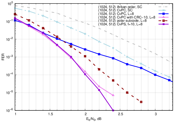
Refer to caption
Fig. 3: Performance of (1024,512)(1024,512) CvPS with f=10f=10 in AWGN channel

In Fig. 3 the performance of (1024,512)(1024,512) CvPS, polar code and polar subcode is presented for f=10f=10 for the case of AWGN channel. The polar code and the polar subcode are constructed for AWGN channel with Eb/N0=2E_{b}/N_{0}=2 dB using Gaussian approximation of density evolution [12], and the CvPS is constructed for the same channel using Monte-Carlo simulations for subchannels qualities. One can see that the CvPS outperforms randomized polar subcodes [10], CvPC [2] and CvPC concatenated with CRC-10.

Refer to caption
Fig. 4: Performance of (4096,2048)(4096,2048) CvPS with f=12f=12 in AWGN channel with Eb/N0=1.25E_{b}/N_{0}=1.25 dB

In Fig. 4 the performance of a (4096,2048)(4096,2048) CvPS with f=12f=12 type-A dynamic frozen symbols is presented. Transmission of BPSK-modulated symbols over AWGN channel with Eb/N0=1.25E_{b}/N_{0}=1.25 dB is considered. The decoding algorithm is the SCL decoding with different values of list size that are shown in the x-axis. The performance of CvPSs is compared to that of a polar subcode with f=12f=12 type-A dynamic frozen symbols and 5252 type-B dynamic frozen symbols. One can see that the CvPS under SCL decoding with the same list size outperforms classical polar subcodes. The smaller list size can be used to achieve the same FER, which allows less sophisticated hardware implementation.

Refer to caption
Fig. 5: SCL decoding complexity of (4096,2048)(4096,2048) CvPS with f=12f=12

In Fig. 5 the complexity (the number of operations) of SCL decoding, based on the expressions derived in [4], of the described above codes is compared for list size L=1​…​64L=1\dots 64 for the CvPS and L=1​…​1024L=1\dots 1024 for the polar subcode. The complexity is obtained as the number of additions and comparisons of LLRs. The complexity of SC decoding for CvPS is approximately 46.5​n​log⁡n46.5n\log n, as shown in [4]. The complexity of SC decoding of polar codes is n​log⁡nn\log n. However, as was shown in [2], CvPT induces stronger polarization than Arikan polarizing transformation, so the smaller list size is needed to achieve the same FER. This leads to the smaller complexity needed to achieve FER less than 6⋅10−46\cdot 10^{-4} in the case of CvPS, because achieving this FER requires list size L=352L=352 for polar subcodes and only L=28L=28 for CvPS. Furthermore, for a large list size the SCL decoding is near-ML, and for sufficiently good channel FER of ML-decoding is mainly defined by the minimum distance and the error coefficient. Dynamic frozen symbols decrease the error coefficient and may even increase the minimum distance of a CvPS. In Fig. 2 one can see that the minimum distance of CvPS is higher than that of CvPC.

VII Conclusions

In this paper a tight lower bound on minimum distance of convolutional polar codes is provided. Furthermore, a generalization of the randomized construction of polar subcodes to the case of convolutional polarizing transformation is proposed. Simulations show that the proposed code construction has lower frame error rate under SCL decoding [4] compared to polar subcodes with the same list size. The complexity for achieving the same FER with convolutional polar subcodes can be lower than in the case of polar subcodes [10] based on Arikan polarizing transformation.

Proof of Theorem 2. For erasure configuration ℰ⊆[n]\mathcal{E}\subseteq[n], denote ℰ′=ℰ∩[n/2]\mathcal{E}^{\prime}=\mathcal{E}\cap[n/2] and ℰ′′={j−n/2∣j∈ℰ∖[n/2]}\mathcal{E}^{\prime\prime}=\left\{j-n/2\mid j\in\mathcal{E}\setminus[n/2]\right\}. We now consider the case of φ=2​ψ+1\varphi=2\psi+1 and prove (19).

Note that u02​ψ=𝟎2​ψ+1u_{0}^{2\psi}=\mathbf{0}^{2\psi+1} implies x0ψ−1=z0ψ−1=𝟎ψx_{0}^{\psi-1}=z_{0}^{\psi-1}=\mathbf{0}^{\psi}. By (3) one obtains

Q^=(X^​Q^′,Z^​Q^′′),\displaystyle\hat{Q}=\left(\hat{X}\hat{Q}^{\prime}\;,\;\hat{Z}\hat{Q}^{\prime\prime}\right),

where Q^=Q[2​ψ+1]¯,ℰ¯(n)\hat{Q}=Q^{(n)}_{\overline{[2\psi+1]},\overline{\mathcal{E}}}, Q^′=Q[ψ]¯,ℰ′¯(n/2)\hat{Q}^{\prime}=Q^{(n/2)}_{\overline{[\psi]},\overline{\mathcal{E}^{\prime}}}, Q^′′=Q[ψ]¯,ℰ′′¯(n/2)\hat{Q}^{\prime\prime}=Q^{(n/2)}_{\overline{[\psi]},\overline{\mathcal{E}^{\prime\prime}}}, X^=X[2​ψ+1]¯,[ψ]¯(n)\hat{X}=X^{(n)}_{\overline{[2\psi+1]},\overline{[\psi]}}, Z^=Z[2​ψ+1]¯,[ψ]¯(n)\hat{Z}=Z^{(n)}_{\overline{[2\psi+1]},\overline{[\psi]}}. By (13), p02∈χn(φ,3)​(ℰ)p_{0}^{2}\in\chi^{(\varphi,3)}_{n}(\mathcal{E}) iff there exists qq:

(p02,𝟎k−3)T=Q^qT=(X^Q^′,Z^Q^′′)qT=X^Q^′q′T+Z^Q^′′q′′T,\displaystyle(p_{0}^{2},\mathbf{0}^{k-3})^{T}=\hat{Q}q^{T}=(\hat{X}\hat{Q}^{\prime},\hat{Z}\hat{Q}^{\prime\prime})q^{T}=\hat{X}\hat{Q}^{\prime}q^{\prime T}+\hat{Z}\hat{Q}^{\prime\prime}q^{\prime\prime T},

where q=(q′,q′′)q=(q^{\prime},q^{\prime\prime}), k=n−φk=n-\varphi, which implies, in particular,

(X^Q^′q′T)[3]¯=(Z^Q^′′q′′T)[3]¯.\displaystyle(\hat{X}\hat{Q}^{\prime}q^{\prime T})_{\overline{[3]}}=(\hat{Z}\hat{Q}^{\prime\prime}q^{\prime\prime T})_{\overline{[3]}}. (22)

Denote a=q′​Q^′Ta=q^{\prime}\hat{Q}^{\prime T}, b=q′′Q^′′Tb=q^{\prime\prime}\hat{Q}^{\prime\prime T}. Thus, a∈cs⁡(Q^′)a\in\cs(\hat{Q}^{\prime}), b∈cs⁡(Q^′′)b\in\cs(\hat{Q}^{\prime\prime}). Then (22) implies a​X^[3]¯,∗T=b​Z^[3]¯,∗Ta\hat{X}_{\overline{[3]},*}^{T}=b\hat{Z}^{T}_{\overline{[3]},*}, so from (4)–(5) one obtains

a​(000000​…100000​…111000​…001110​……)=b​(000000​…100000​…011000​…000110​……),\displaystyle a\begin{pmatrix}000000\ldots\\ 100000\ldots\\ 111000\ldots\\ 001110\ldots\\ \dots\end{pmatrix}=b\begin{pmatrix}000000\ldots\\ 100000\ldots\\ 011000\ldots\\ 000110\ldots\\ \dots\end{pmatrix},

which leads to the system of equations

{ai+ai+1=bi,i=1​…​n/2−ψ−2ai=bi,i=2​…​n/2−ψ−1\displaystyle\begin{cases}a_{i}+a_{i+1}=b_{i},&i=1\ldots n/2-\psi-2\\ a_{i}=b_{i},&i=2\ldots n/2-\psi-1\end{cases} (23)

It is easy to see that (23) implies ai=bi=0a_{i}=b_{i}=0 for i≥3i\geq 3. Let k′=n/2−ψk^{\prime}=n/2-\psi. By above consideration, for any p∈𝔽3p\in\mathbb{F}^{3} one has (p,𝟎k−3)∈cs⁡(Q^)(p,\mathbf{0}^{k-3})\in\cs(\hat{Q}) iff there exists p′,p′′∈𝔽3p^{\prime},p^{\prime\prime}\in\mathbb{F}^{3}, s.t. (p′,𝟎k′−3)∈cs⁡(Q^′)(p^{\prime},\mathbf{0}^{k^{\prime}-3})\in\cs(\hat{Q}^{\prime}), (p′′,𝟎k′−3)∈cs⁡(Q^′′)(p^{\prime\prime},\mathbf{0}^{k^{\prime}-3})\in\cs(\hat{Q}^{\prime\prime}), and

(p,𝟎3)T=(100110010011001001)​(p′)T+(100100010010001001)​(p′′)T.\displaystyle(p,\mathbf{0}^{3})^{T}=\begin{pmatrix}100\\ 110\\ 010\\ 011\\ 001\\ 001\end{pmatrix}(p^{\prime})^{T}+\begin{pmatrix}100\\ 100\\ 010\\ 010\\ 001\\ 001\end{pmatrix}(p^{\prime\prime})^{T}. (24)

Note that two last elements of vector in the left-hand side equals 00, and two last rows in the right hand size of (24) are identical, so last rows of these matrices can be removed. The resulting matrices are equal to X[1]¯,∗(6)X^{(6)}_{\overline{[1]},*} and Z[1]¯,∗(6)Z^{(6)}_{\overline{[1]},*}, respectively. Recalling (13), one obtains that χn(2​ψ+1,3)​(ℰ)\chi_{n}^{(2\psi+1,3)}(\mathcal{E}) consists of all p02p_{0}^{2}, for which there exist p′∈χn/2(ψ,3)​(ℰ′){p^{\prime}}\in\chi_{n/2}^{(\psi,3)}(\mathcal{E}^{\prime}), p′′∈χn/2(ψ,3)​(ℰ′′)p^{\prime\prime}\in\chi_{n/2}^{(\psi,3)}(\mathcal{E}^{\prime\prime}):

(p02,𝟎2)T=X[1]¯,∗(6)p′T+Z[1]¯,∗(6)p′′T.\displaystyle(p_{0}^{2},\mathbf{0}^{2})^{T}=X^{(6)}_{\overline{[1]},*}p^{\prime T}+Z^{(6)}_{\overline{[1]},*}p^{\prime\prime T}. (25)

Observe that (25) is equivalent to the equation in the right-hand side of (17). Obviously, |ℰ|=|ℰ′|+|ℰ′′||\mathcal{E}|=|\mathcal{E}^{\prime}|+|\mathcal{E}^{\prime\prime}| and the minimal cardinality of (𝒯l,2​ψ+1,3)(\mathcal{T}_{l},2\psi+1,3)-configuration |ℰ||\mathcal{E}| for each 𝒯l∈𝕊3\mathcal{T}_{l}\in\mathbb{S}_{3} can be found exactly as it is stated in (19).

Equality (20) can be proved similarly.

References

  • [1] A. J. Ferris and D. Poulin, “Branching MERA codes: a natural extension of polar codes,” CoRR, vol. abs/1312.4575, 2013. [Online]. Available: http://arxiv.org/abs/1312.4575
  • [2] A. J. Ferris, C. Hirche, and D. Poulin, “Convolutional polar codes,” CoRR, vol. abs/1704.00715, 2017. [Online]. Available: http://arxiv.org/abs/1704.00715
  • [3] E. Arikan, “Channel polarization: A method for constructing capacity-achieving codes for symmetric binary-input memoryless channels,” IEEE Transactions on Information Theory, vol. 55, no. 7, pp. 3051–3073, July 2009.
  • [4] R. Morozov and P. Trifonov, “Efficient SC decoding of convolutional polar codes,” in 2018 International Symposium on Information Theory and its Applications (ISITA2018), Singapore, Singapore, Oct. 2018.
  • [5] H. Saber, Y. Ge, R. Zhang, W. Shi, and W. Tong, “Convolutional polar codes: LLR-based successive cancellation decoder and list decoding performance,” in 2018 IEEE International Symposium on Information Theory (ISIT), June 2018, pp. 1480–1484.
  • [6] T. Prinz and P. Yuan, “Successive cancellation list decoding of BMERA codes with application to higher-order modulation,” in 2018 International Symposium on Turbo Codes and Iterative Information Processing (ITW), December 2018.
  • [7] N. Hussami, S. B. Korada, and R. Urbanke, “Performance of polar codes for channel and source coding,” in Proceedings of IEEE International Symposium on Information Theory, 2009, pp. 1488–1492.
  • [8] A. Canteaut and F. Chabaud, “A new algorithm for finding minimum-weight words in a linear code: Application to McEliece’s cryptosystem and to narrow-sense BCH codes of length 511511,” IEEE Transactions on Information Theory, vol. 44, no. 1, pp. 367–378, January 1998.
  • [9] B. Li, H. Shen, and D. Tse, “An adaptive successive cancellation list decoder for polar codes with cyclic redundancy check,” IEEE Communications Letters, vol. 16, no. 12, pp. 2044–2047, December 2012.
  • [10] P. Trifonov and G. Trofimiuk, “A randomized construction of polar subcodes,” in Proceedings of IEEE International Symposium on Information Theory. IEEE, 2017, pp. 1863–1867.
  • [11] I. Tal and A. Vardy, “List decoding of polar codes,” IEEE Transactions On Information Theory, vol. 61, no. 5, pp. 2213–2226, May 2015.
  • [12] P. Trifonov, “Efficient design and decoding of polar codes,” IEEE Transactions on Communications, vol. 60, no. 11, pp. 3221 – 3227, November 2012.