Feature Pyramid and Hierarchical Boosting Network for Pavement Crack Detection
Abstract
Pavement crack detection is a critical task for insuring road safety. Manual crack detection is extremely time-consuming. Therefore, an automatic road crack detection method is required to boost this progress. However, it remains a challenging task due to the intensity inhomogeneity of cracks and complexity of the background, e.g., the low contrast with surrounding pavements and possible shadows with similar intensity. Inspired by recent advances of deep learning in computer vision, we propose a novel network architecture, named Feature Pyramid and Hierarchical Boosting Network (FPHBN), for pavement crack detection. The proposed network integrates context information to low-level features for crack detection in a feature pyramid way. And, it balances the contributions of both easy and hard samples to loss by nested sample reweighting in a hierarchical way during training. In addition, we propose a novel measurement for crack detection named average intersection over union (AIU). To demonstrate the superiority and generalizability of the proposed method, we evaluate it on five crack datasets and compare it with state-of-the-art crack detection, edge detection, and semantic segmentation methods. Extensive experiments show that the proposed method outperforms these methods in terms of accuracy and generalizability. Code and data can be found in https://github.com/fyangneil/pavement-crack-detection
Index Terms:
Pavement crack detection, deep learning, feature pyramid, hierarchical boosting.I Introduction
Crack is a common pavement distress, which is a potential threat to road and highway safety. To maintain the road in good condition, localizing and fixing the cracks is a vital responsibility for transportation maintenance department. One major step of the task is crack detection. However, manual crack detection is considerably tedious and requires domain expertises. To alleviate the workload of expertisers and facilitate the progress of road inspection, it is necessary to achieve automatic crack detection.
With the development of technologies in computer vision, numerous efforts have been devoted to applying computer vision technologies to perform automatic crack detection [1, 2, 3, 4, 5, 6, 7]. In early days, Liu et al [8] and Kaseko et al [6] use threshold-based approaches to find crack regions based on the assumption that real crack pixel is consistently darker than its surroundings. Currently, most of the methods are based on hand crafted feature and patch-based classification. Many types of such features have been used for crack detection such as: Gabor filters [9][10], wavelet features [11], Histogram of Oriented Gradient (HOG) [12], and Local Binary Pattern (LBP) [13]. These methods encode the local pattern but lack global view of crack. To conduct crack detection from a global view, some works [14, 4, 15] carry out crack detection by taking into account photometric and geometric characteristics of pavement crack images. These methods partially eliminate noises and enhance continuity of detected cracks.
While these methods perform crack detection in a global view, their detection performance are not superior when dealing with cracks with intensity inhomogeneity or complex topology. The failures of these methods can be attributed to lacking robust feature representation and ignoring interdependency among cracks.

To overcome the aforementioned shortcomings, CrackForest [2] incorporates complementary features from multiple levels to characterize cracks and takes advantage of the structural information in crack patches. This method is shown to outperform state-of-the-art crack detection methods like CrackTree [4], CrackIT [17], Free-Form Anisotropy (FFA) [18], and Minimal Path Selection (MPS)[14]. However, CrackForest [2] still performs crack detection based on hand crafted feature, which is not discriminative enough to differentiate the cracks from complex background with low level cues.

Recently, deep learning has been widely applied in computer vision for its excellent representation capability. Some works [1] [19] [20] [5] have been devoted to leverage this property of deep learning to learn robust feature representation for crack detection. Zhang et al[1], Pauly et al [19], and Eisenbach et al [20] use deep learning to perform patch-based classification for crack detection, which is inconvenient and sensitive to patch scale. Schmugge et al [5] treats crack detection as a segmentation task, which classifies each pixel as crack or background category using deep learning. Although [5] gains decent performance, crack detection is very different from semantic segmentation in terms of ratio of foreground and background. In semantic segmentation, the foreground and background are not as unbalanced as those in crack detection.
In contrast, crack detection task is more similar to edge detection in terms of the foreground to background ratio. In addition, crack and edge detection share similar characteristics in shape and structure. Due to these common characteristics, it is intuitive to adopt edge detection methods to crack detection. For instance, Shi et al [2] successfully apply structure forest[21], a classical edge detection method, for crack detection. However, this approach is based on hand crafted features, lacking of representative ability.
To learn robust feature representation and to cope with the highly skewed classes problem for automatic crack detection, we propose a Feature Pyramid and Hierarchical Boosting Network (FPHBN) to automatically detect crack in an end-to-end way. FPHBN adopts Holistically-nested Edge Detection (HED) [16], a breakthrough edge detection method, as its backbone architecture.
Fig. 1 shows the architecture configuration of HED [16] and the proposed FPHBN. The difference is that FPHBN integrates a feature pyramid module and a hierarchical boosting module into HED[16]. The feature pyramid is built through a top-down architecture to introduce context information from higher-level to lower-level feature maps. This can enhance feature representation in lower-level layers, leading to a representative capability improvement to distinguish the crack from background. The hierarchical boosting is proposed to reweight samples from top layer to bottom layer, which makes the FPHBN pay more attention to hard examples.
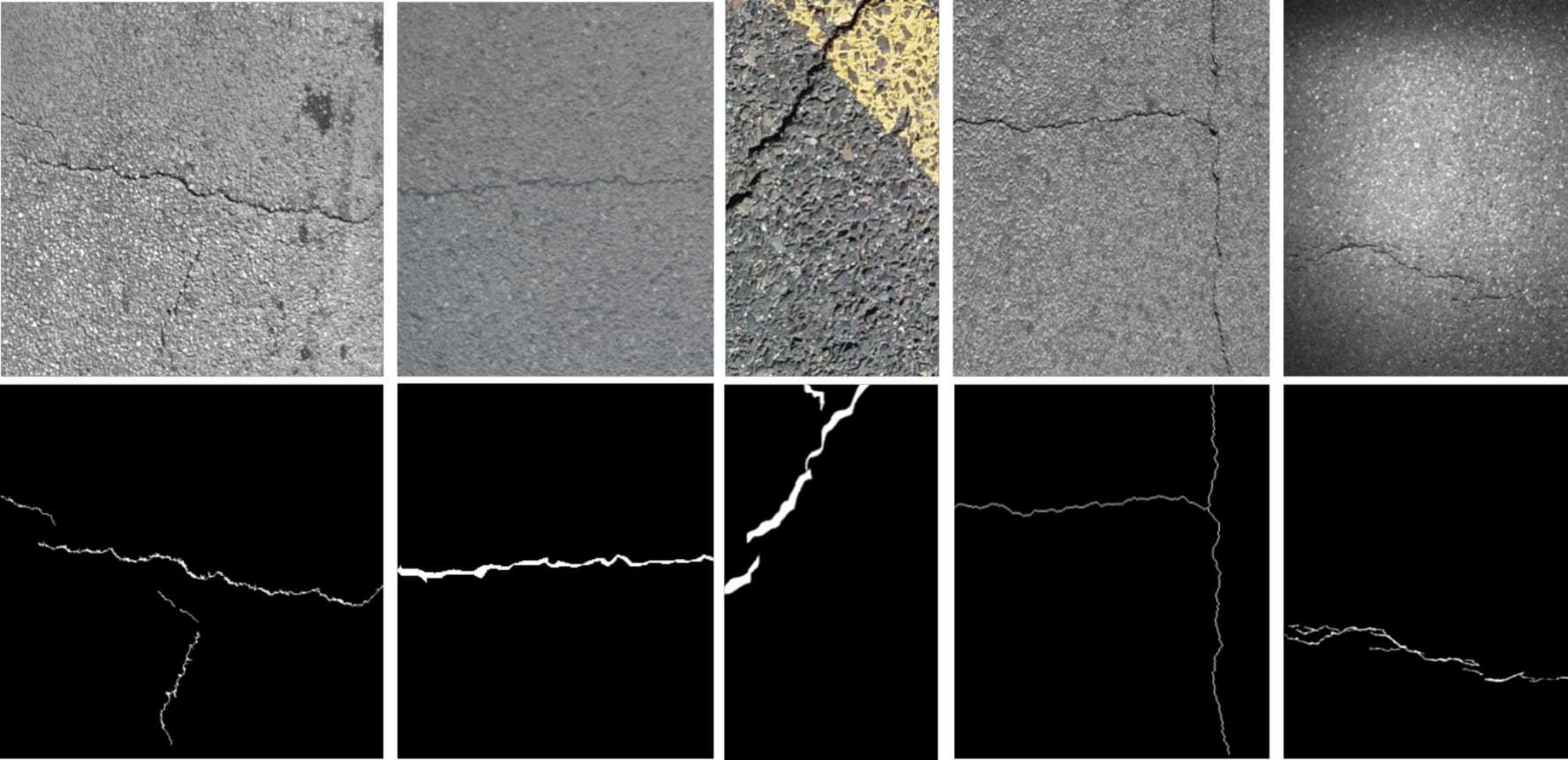
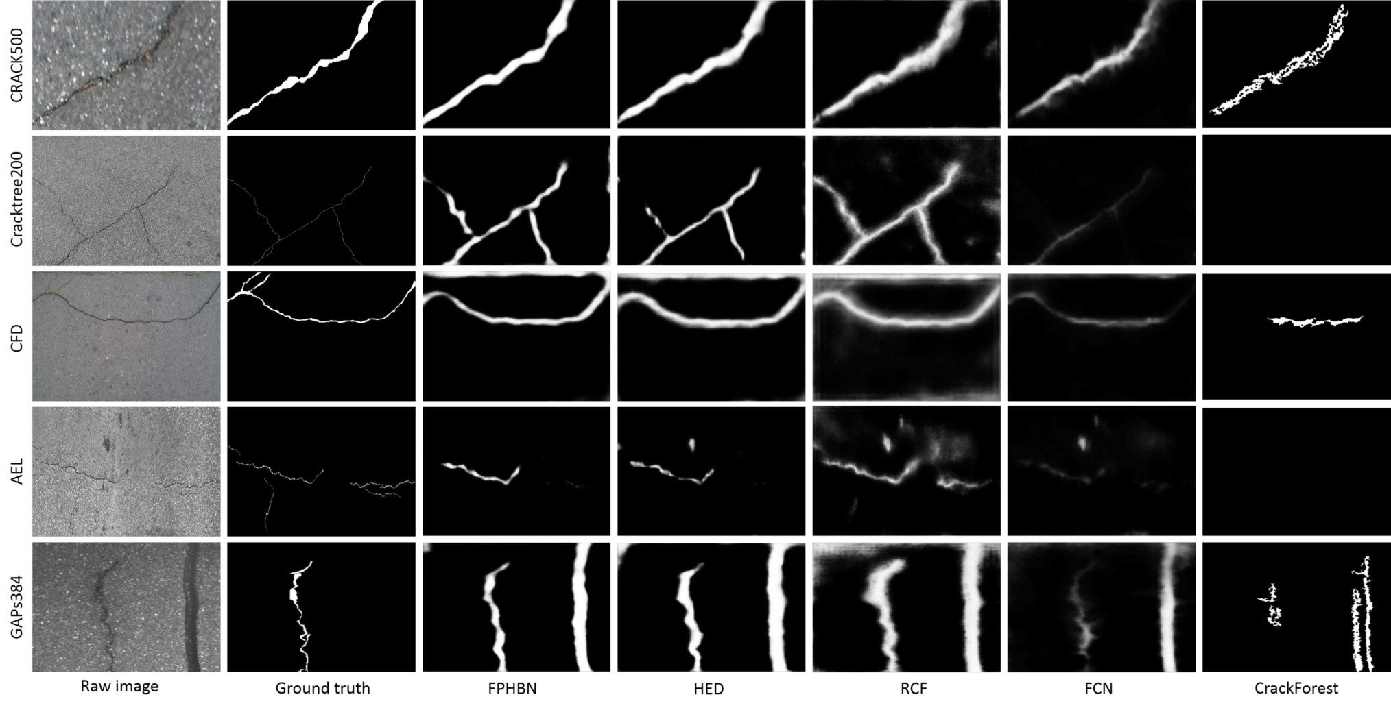
Fig. 2 shows the detection results of FPHBN and state-of-the-art edge and semantic segmentation methods: HED [16], Richer Convolutional Features for edge detection (RCF)[22], Fully Convolutional Networks for semantic segmentation (FCN)[23]. From Fig. 2, we can see that detection result of FPHBN is much clearer than those of other methods and has less false positives.
To evaluate crack detection algorithms, Shi et al [2] use precision and recall (PR) as measurements. The detected pixels are treated as true positives if these pixels locate within five pixels from labeled pixels. This criterion is too loose when the crack annotation is with a large width. Moreover, PR cannot appropriately demonstrate the overlapping extent between detected crack and ground truth, especially when crack is large. For example, in Fig. 3, we see that ground truth in the third column is much wider than others. In this situation, PR is not precise enough to measure the detection results. Thus in addition to PR, we propose average intersection over union (AIU) as a complementary measurement for evaluating crack detection. By computing the average intersection over union (IU) over different thresholds, AIU takes the width information into consideration to evaluate detections and illustrates the overall overlap extent between detections and ground truth. Thus the AIU can be used to determine if the width is precisely estimated, which is critical to assess the damage degree of pavement.
The contributions of this paper can be summarized in the following aspects:
- •
A feature pyramid module is introduced for crack detection. The feature pyramid is constructed by a top-down architecture which incorporates context information from top to bottom, layer by layer.
- •
A hierarchical boosting module is proposed to reweight samples layer by layer so as to make the model focus on hard samples.
- •
A new measurement is proposed to evaluate crack detection methods. The measurement not only takes into account the crack width, but also avoids the annotation bias.
II Related works
In this section, we first briefly review traditional works on crack detection. Then, deep learning-based crack detection methods are discussed to demonstrate their superiority to traditional approaches.
II-A Traditional crack detection methods
In this work, we refer to as traditional crack detection methods the crack detection methods that are based on non-deep learning techniques. Over the past years, numerous researchers have been devoted to automating crack detection. These works can be divided into five categories: 1) wavelet transform, 2) image thresholding, 3) hand crafted feature and classification, 4) edge detection-based methods, and 5) minimal path-based methods.
II-A1 Wavelet transform

In [11], a wavelet transform is applied to a pavement image, such that the image is decomposed into different frequency subbands. The distresses and noise are transformed into high and low amplitude wavelet coefficients, respectively. Subirats et al [24] build a complex coefficient map by performing a 2D wavelet transform in a multi-scale way; then crack region can be obtained by searching the maximum wavelet coefficients from largest to smallest scale. However, these approaches cannot deal with cracks with low continuity or high curvature property since the anisotropic characteristic of wavelet.
II-A2 Image thresholding
In [25, 26, 27, 28], preprocessing algorithms are first used to reduce the illumination artifacts. Then thresholding is applied to the image to yield crack candidates. The processed crack image is further refined using morphological technologies. [4] [15] [29] are variants of this group, which leverage graph-based methods for crack candidates refinement.
II-A3 Hand crafted feature and classification
II-A4 Edge detection-based methods
Yan et al [33] introduce morphological filters into crack detection and removes noise with a modified median filter. Ayenu-Prah et al [34] apply Sobel edge detector to detect crack after smoothing image and removing speckle noise by a bidimensional empirical mode decomposition algorithm. Shi et al [2] apply random structure forest [21] to exploit structural information for crack detection.
II-A5 Minimal path-based methods
Kass et al [35] propose to use minimal path method to extract simple open curves in images for given both endpoints of a curve. Kaul et al[36] propose to detect same type of contour-like image structures using an improved minimal path method. The improved method needs less prior knowledge of both topology and endpoints of the desired curves. Amhaz et al[14] propose a two-stage method for crack detection: first select endpoint at local scale; second select minimal paths at global scale. Nguyen et al[18] present a method to take into account intensity and crack shape features for crack detection simultaneously by introducing Free-Form Anisotropy[18].
II-B Deep learning-based crack detection
Recent years, deep learning achieves unprecedented success in computer vision [37]. A lot of works try to apply deep learning to crack detection task. Zhang et al [1] first propose a relatively shallow neural network, consisting of four convolutional layers and two fully connected layers, to perform crack detection in a patch-based way. Moreover, Zhang et al [1] compare their method with hand crafted feature based methods to demonstrate the advantages of feature representation of deep learning. Pauly et al[19] apply a deeper neural network to classify crack and non-crack patches and demonstrates the superiority of deeper neural network. Feng et al[38] propose a deep active learning system to deal with limited label resources problem. Eisenbach et al [20] present a road distress dataset for training deep learning network and first evaluates and analyzes state-of-the-art approaches in pavement distress detection.
The aforementioned approaches treat crack detection as a patch-based classification task. Each image is cropped to small patches, then a deep neural network is trained to classify each patch as crack or not. This way is inconvenient and sensitive to patch scale. Due to the rapid development in semantic segmentation task [23] [39][40], Schmugge et al [5] present a crack segmentation method based on SegNet [39] for remote visual examination videos. This method performs crack detection by aggregating the crack probability from multiple overlapping frames in a video.
III method
III-A Overview of proposed method
In this paper, crack detection is formulated as a pixel-wise binary classification task. For a given crack image, a designed model yields a crack prediction map, where crack regions have higher probability and non-crack regions have lower probability. Fig. 4 shows the architecture of the proposed Feature Pyramid and Hierarchical Boosting Network (FPHBN). FPHBN is composed of four major components: 1. a bottom-up architecture for hierarchical feature extraction, 2. a feature pyramid for merging context information to lower layers using a top-down architecture, 3. side networks for deep supervision learning, and 4. a hierarchical boosting module to adjust sample weights in a nested way.

Given a crack image and corresponding ground truth, the crack image is first fed into the bottom-up network to extract features of different levels. Each conv layer corresponds to a level in the pyramid. At each level, except for the fifth one, a feature merging operation is conducted to incorporate higher-level feature maps to lower-level ones layer-by-layer to make context information flow from higher to lower ones. At each level the feature maps in top-down architecture are fed to a convolutional filter of size for dimension reduction and a de-convolutional filter to resize feature map to the same size of the input image. Then each resized feature map is introduced to the hierarchical boosting module to yield crack prediction map and compute sigmoid cross-entropy loss with ground truth. The convolutional filter, de-convolutional filter, and loss layer at each level comprise a side network. Finally, all the five resized feature maps are fused together by a concatenate layer followed by a convolutional filter to produce a crack prediction map and compute a final sigmoid cross-entropy loss with ground truth.
III-B Bottom-up architecture
In our method, the bottom-up architecture consists of the conv1-conv5 parts of VGG [41] including max pooling layers between convolutional layers. Through the bottom-up architecture, convolutional networks (ConvNets) compute a hierarchical feature representation. Due to the max pooling layers, the feature hierarchy has an inherent multi-scale, pyramid shape.
Unlike multi-scale features built upon multi-scale images, the multi-scale feature computed by deep ConvNets is more robust to variance in scale[42]. Thus it facilitates recognition on a single input scale. More importantly, deep ConvNets make the progress of producing multi-scale representation automated and convenient. This is much more efficient and effective than computing engineered features on various scales of images.
In the bottom-up network, the in-network hierarchy produces feature maps of different spatial resolutions, but introduces large context gaps. The bottom levels of feature maps are of higher resolution but have less context information than top levels of features. In contrast, the top levels of feature maps are lower resolution but have more context information. The context information is helpful for crack detection. Therefore, if these feature maps are directly fed into each side network, the output from different side network varies significantly.
The first row in Fig. 5 shows the five side outputs and fused output. We note that the side outputs 1-3 are very messy and hardly recognized; the side outputs 4-5 and fused are much better than the side outputs 1-3. In addition, we find that although fused result is clearer than side outputs 1-4, it is still a little blur. This is because fused result merges the information from the side outputs 1-4, which is cluttered and blur. The reason causes these messy side outputs is that the lower-level layers lack context information.
III-C Feature pyramid

To deal with the aforementioned issue, we introduce context information to lower-level layers to generate a feature pyramid through a top-down architecture, which is inspired by [42]. As shown in Fig. 4, the top-down architecture feeds the fifth and fourth levels of feature maps into a feature merging operation unit, then feeds the output and third level of feature maps to next merging operation unit. This operation is conducted progressively until the bottom level. In this way, we produce a set of new feature maps, which contain much richer features at each level than that in bottom-up network except for fifth level. From Fig. 5, we note that after introducing feature pyramid, the side outputs 1-4 and fused result are significantly clearer than counterparts from HED [16]. Combining multi-scale context information into low-level feature maps by the feature pyramid module benefits the performance improvement of low-level side networks. Specifically, detecting various scales of crack requires different extents of context information. Since the deeper convolution layers have much larger receptive fields than the shallower ones, the high-level features contain more context information than the low-level ones. Therefore, when high-level features are combined with low-level ones, the low-level side networks utilize the multi-scale context information to increase its detection performance and to boost the fused detection performance.
The feature merging operation of the feature pyramid is illustrated in Fig. 6. We use the feature merging operation at the fourth level as an example to demonstrate the concrete operations. The feature maps from conv5 are upsampled twice and concatenated with the feature maps from conv4. The concatenated feature maps are fused and reduced by a convolutional layer of 512 filters. Note that from conv3 to conv1 level, the filter number is set to 256, 128, and 64, respectively.
III-D Side networks
The side network at each level performs crack prediction individually. This configuration of learning is named as deeply supervised learning, proposed in [43] and justified considerably useful for edge detection in HED [16]. The key characteristic of the deep supervision is that instead of performing recognition task at the highest layer, the recognition is conducted at each level through the side network. Let us first introduce HED [16] in the context of crack detection.
III-D1 Training Phase
We denote our crack training dataset as , where sample and denote the raw crack image and the corresponding binary ground truth crack map, respectively. For convenience, we drop the subscript in subsequent paragraphs. The parameters of the entire network are denoted as . Assume there are side networks in HED[16]. Each side network is associated with a classifier, in which the corresponding weights are denoted as . The objective function is defined as
| (1) |
where represents the image-level loss function for a side network. During the image-to-image training, the loss function is computed over all pixels in a training image and crack map . However, this kind of loss function regards positives and negatives equally, which is not suited for practical situation. For a typical crack image, as shown in Fig. 5, the distribution of crack and non-crack pixels is heavily biased. Most regions of the image are non-crack pixels. HED[16] uses a simple strategy to automatically balance the contribution to the loss from positives and negatives. A class-balancing weight is introduced in a pixel-wise way. Index is over the image spatial dimensions of image . Then is used to offset the imbalance between crack and non-crack pixels. Specifically, Equation 1 is rewritten as
| (2) | |||
where and . and denote the crack and non-crack pixels in ground truth image, respectively. is computed by a sigmoid function on the activation at pixel . At each side output network, we then obtain crack map predictions , where are activations of the side output of layer .
To leverage the side output prediction, a ‘weighted-fusion’ layer is added to the network and simultaneously learns the fusion weight with all side networks during training. The loss function of the fusion layer becomes
| (3) |
where where is the fusion weight. is the distance between the fused predictions and the ground truth crack map, which is set to a sigmoid cross-entropy loss. For the entire network, the overall object function needs to be minimized is
| (4) |
III-D2 Test Phase
During testing, for image , a set of crack map predictions are yielded from both side network and the fusion layer:
| (5) |
where CNN(.) denotes the crack maps generated by HED[16].
III-E Hierarchical boosting
Although HED [16] takes into account the issue of unbalanced positives and negatives by using a class-balancing weight , it cannot differentiate easy and hard samples. Specifically, in crack detection, the loss function Equation 4 is dominated by easily classified negative samples since the samples are highly skewed. Thus, the network cannot effectively learn parameters from misclassified samples during training phase.
To address this problem, a common solution is to perform some forms of hard mining [44][45] that samples hard samples during training or more complex sampling/reweighting schemes [46]. In contrast, Lin et al [47] propose a novel loss to down-weight well-classified examples and focus on hard examples during training.
Different from these previous works, we design a new scheme, hierarchical boosting, to reweight samples. From Fig. 4, we note that in the hierarchical boosting module, from top to bottom, a sample reweighting operation is conducted layer by layer. This top-down hierarchical is inspired by the observation that in Fig. 5 the side output predictions are similar with each other. This means each side network has similar capability for crack detection. In addition, the five side networks are sequential in terms of information flowing. For example, the fourth side network needs the feature maps from the fifth side network to compute crack prediction map and loss. If the upper network can inform lower network which samples are hard to classify, the lower networks will pay more attention to these hard samples. Through this communication, crack detection performance can be improved. Therefore, we propose the hierarchical boosting method to deal with the hard sample problem by facilitating communication between adjacent side networks.
Specifically, given the output from the th side network, the difference between and ground truth is denoted as . Thus, the loss function Equation 2 of the -th side network can be rewritten to
| (6) | |||
where is the difference at pixel , is integer and . Thus, the prediction of deeper side network is leveraged to weight loss term in the shallower side network to encourage the communication among different side networks.
IV Experiments and Results
In this section, we describe the implementation details of the proposed FPHBN. Then datasets for evaluation, compared methods, and evaluation criteria are introduced. Finally, we present and analyze experimental results.
IV-A Implementation details
The proposed method is implemented on the widely used Caffe library [48] and an open implementation of FCN[23]. The bottom-up part is the conv1-conv5 of pretrained VGG [41]. The feature pyramid is implemented by using Concat and Convolutional layers in Caffe. Sample reweighting is implemented using python.
IV-A1 Parameters setting
The hyperparameters include: mini-batch (10), learning rate (1e-8), loss weight of each side network (1), momentum (0.9), weight decay (0.0002), initialization of the each network (0), initialization of fusion layer (0.2), initialization of filters in feature merging operation (Gaussian kernel with mean 0 and std 0.01), the number of training iteration (40,000), learning rate divided by 10 per 10,000 iterations. The model is saved every 4,000 iterations.
IV-A2 Upsampling operation
Within the proposed FPHBN, the upsampling operations are implemented with in-network de-convolutional layers. Instead of learning the parameters of de-convolutional layers, we freeze the parameters to perform bilinear interpolation.
IV-A3 Sample reweighting
For sample reweighting, as there is no layer in Caffe to complete such function, we implement it with a python layer and integrate it to the proposed network using python Caffe interface. To make sure the performance gained is not caused by our implementation, we first conduct experiments using our implemented class-imbalance cross-entropy loss and compare it with the original implementation. We find that the experimental results are same.
IV-A4 Computation platform
At inference phase, deep learning based methods are tested on a 12G GeForce GTX TITAN X. Non-deep learning method is tested on a computer with 16G RAM and i7-3770 CPU@3.14GHz.
IV-B Datasets
IV-B1 CRACK500
We collect a pavement crack dataset with 500 images of size around pixels on main campus of Temple University using cell phones. This dataset is named as CRACK500. Each crack image has a pixel-level annotated binary map. To facilitate future research, we share the CRACK500 to the research community, To our best knowledge, this dataset is currently the largest publicly accessible pavement crack dataset with pixel-wise annotation. The dataset is divided into 250 images of training data, 50 images of validation data, and 200 images of test data.
Due to limited number of images, large size of each image, and restricted computation resource, we crop each image into 16 non-overlapped image regions and only the region containing more than 1,000 pixels of crack is kept. Through this way, the training data consists of 1,896 images, validation data contains 348 images, test data contains 1124 images. The validation data is used to choose the best model during training process to prevent overfitting. Once the model is chosen, it is tested on the test data and other datasets for generalizability evaluation.
IV-B2 GAPs384
German Asphalt Pavement Distress (GAPs) dataset is presented in [20] to address the issue of comparability in the pavement distress domain by providing a standardized high-quality dataset of large scale. The GAPs dataset includes a total of 1,969 gray valued images, with various classes of distress such as cracks, potholes, inlaid patches, et. al. The image resolution is pixels with a per pixel resotution of . For more details of the dataset, the readers are referred to [20]
The actual damage in an image is enclosed by a bounding box. This type of annotation is not fine enough to training deep model for a pixel-wise crack prediction task. To address this problem, we manually select 384 images from the GAPs dataset, which only includes crack class of distress, and conduct pixel-wise annotation. This pixel-wise annotated crack dataset is named as GAPs384 and used to test the generalization of the model trained on CRACK500.
Due to the large size of image and limited memory of GPU, each image is cropped to 6 non-overlapped image regions of size pixels. Only the image regions with more than pixels are remained. Thus we gain 509 images for test.
IV-B3 Cracktree200
Zou et al[4] present a dataset to evaluate their proposed method. The dataset includes 206 pavement images of size with various types of cracks. Therefore, we name this dataset as Cracktree200. This dataset is with challenges like shadows, occlusions, low contrast, noise, etc. The annotation of the dataset is pixel-wise label, which can be directly used for evaluation.
IV-B4 CFD
Shi et al[2] propose an annotated road crack dataset called CFD. The dataset consists of 118 images of size pixels. Each image has manually labeled crack contours. The device used to acquire the images is an iPhone5 with focus of 4mm, aperture of f/2.4 and exposure time of 1/135s. The CFD is used for evaluating model.
IV-B5 Aigle-RN & ESAR & LCMS
Aigle-RN is proposed in [14], which contains 38 images with pixel-level annotations. The dataset is acquired at traffic speed for periodically monitoring the French pavement surface condition using Aigle-RN system. ESAR is acquired by a static acquisition system with no controlled lighting. ESAR has 15 fully annotated crack images. LCMS contains 5 pixel-wise annotated crack images. Since the three datasets have small number of images, they are combined to one dataset named AEL for model evaluation.
IV-C Compared methods
IV-C1 HED
IV-C2 RCF
IV-C3 FCN
IV-C4 CrackForest
We train CrackForest[2] on CRACK500 training data. All the hyperparameters are set as default.

IV-D Evaluation criteria
Since the similarity with edge detection, it is intuitive to directly leverage criteria of edge detection to conduct evaluation for crack detection. The standard criteria in edge detection domain are the best F-measure on the data set for a fixed scale (ODS), the aggregate F-measure on the data set for the best scale in each image (OIS).
The definitions of the ODS and OIS are and . The denotes the threshold, is the index of image, is the total number of images. and are precision and recall at threshold over dataset. and are computed over image . For the detailed definition of the two criteria, the readers are referred to [49]. The edge ground truth annotation is a binary boundary map, which is different from the ground truth annotation in some crack datasets, where crack annotation is a binary segmentation map. Therefore, during evaluation both crack detection and ground truth are first processed by non-max suppression (NMS), then thinned to one pixel wide before computing ODS and OIS. Note that the maximum tolerance allowed for correct matches of prediction and ground truth is set to 0.0075.
The proposed new measurement, AIU, is computed on the detection and ground truth without NMS and thinning operation. AIU of an image is defined as
| (7) |
where denotes the total number of thresholds with interval ; for a given threshold t, is the number of pixels of intersected region between the predicted and ground truth crack area; and denote the number of pixels of predicted and ground truth crack region, respectively. Thus the AIU is in the range of 0 to 1, the higher value means the better performance. The AIU of a dataset is the average of the AIU of all images in the dataset.

| Methods | AIU | ODS | OIS | time/image (s) |
| HED[16] | 0.481 | 0.575 | 0.625 | 0.067 (GPU) |
| RCF [22] | 0.403 | 0.490 | 0.586 | 0.066 (GPU) |
| FCN[23] | 0.379 | 0.513 | 0.577 | 0.101 (GPU) |
| CrackForest [2] | N/A | 0.199 | 0.199 | 2.951 (CPU) |
| FPHBN | 0.489 | 0.604 | 0.635 | 0.197 (GPU) |
IV-E Experimental results
IV-E1 Results on CRACK500
On CRACK500, we use the validation data to select the best training iteration. From Fig. 7, we can note that the AIU metric tends to converge over the training iterations. Based on the curve, we choose the model when its AIU curve has converged. In other word, FPHBN, HED[16], and RCF[22] are chosen at 12,000th iteration, FCN[23] is chosen at 36,000th iteration. From TABLE I, we see that on validation dataset FPHBN surpasses RCF[22], HED[16], and FCN[23] in terms of AIU.
We explore the contributions of each component of the proposed method on the validation set of CRACK500. As shown in TABLE I, we first introduce Feature Pyramid to HED, i.e., HED-FP. Compared with the original HED, we observe that the AIU improves from 0.541 to 0.553. We then integrate the Hierarchical Boosting into HED-FP, i.e., FPHBN. The AIU increases from 0.553 to 0.560 compared with HED-FP. Both the Feature Pyramid and Hierarchical Boosting contribute to the improvement of the performance.
On the Crack500 test dataset, the evaluation curves and detection results of compared methods are shown in the first column of Fig. 8 and the first row of Fig. 9, respectively. For intersection over union (IU) curve, we see that FPHBN always has considerably promising IU over various thresholds. For precision and recall (PR) curve, FPHBN is the highest among all compared methods. Since the output of CrackForest [2] is a binary map, we cannot compute the IU and PR curve and just list the ODS and OIS value in related tables.
As shown in TABLE II, FPHBN improves the performance by relative to HED[16], second best, in terms of ODS. In the first row of Fig. 9, we note that FPHBN gains visually much clearer crack detections than others.

IV-E2 Results on GAPs384
| Methods | AIU | ODS | OIS | time/image (s) |
| HED[16] | 0.069 | 0.209 | 0.175 | 0.086 (GPU) |
| RCF [22] | 0.043 | 0.172 | 0.120 | 0.083 (GPU) |
| FCN[23] | 0.015 | 0.088 | 0.091 | 0.119 (GPU) |
| CrackForest [2] | N/A | 0.126 | 0.126 | 4.101 (CPU) |
| FPHBN | 0.081 | 0.220 | 0.231 | 0.241 (GPU) |
| Methods | AIU | ODS | OIS | time/image (s) |
| HED[16] | 0.040 | 0.317 | 0.449 | 0.130(GPU) |
| RCF[22] | 0.032 | 0.255 | 0.487 | 0.128 (GPU) |
| FCN[23] | 0.008 | 0.334 | 0.333 | 0.166 (GPU) |
| CrackForest [2] | N/A | 0.080 | 0.080 | 5.091 (CPU) |
| FPHBN | 0.041 | 0.517 | 0.579 | 0.377 (GPU) |
| Methods | AIU | ODS | OIS | time/image (s) |
| HED[16] | 0.154 | 0.593 | 0.626 | 0.047 (GPU) |
| RCF[22] | 0.105 | 0.542 | 0.607 | 0.040 (GPU) |
| FCN[23] | 0.021 | 0.585 | 0.609 | 0.07 (GPU) |
| CrackForest [2] | N/A | 0.104 | 0.104 | 3.742 (CPU) |
| FPHBN | 0.173 | 0.683 | 0.705 | 0.133 (GPU) |
| Methods | AIU | ODS | OIS | time/image (s) |
| HED[16] | 0.075 | 0.429 | 0.421 | 0.098 (GPU) |
| RCF[22] | 0.069 | 0.469 | 0.397 | 0.097 (GPU) |
| FCN[23] | 0.022 | 0.322 | 0.265 | 0.128 (GPU) |
| CrackForest [2] | N/A | 0.231 | 0.231 | 2.581 (CPU) |
| FPHBN | 0.079 | 0.492 | 0.507 | 0.259 (GPU) |
| Method | ODS (meanstd) | OIS (meanstd) |
|---|---|---|
| HED[16] | 0.387 0.164 | 0.418 0.186 |
| RCF[22] | 0.3590.175 | 0.403 0.207 |
| FCN[23] | 0.3320.203 | 0.325 0.215 |
| CrackForest [2] | 0.1350.067 | 0.1350.067 |
| FPHBN | 0.4780.192 | 0.505 0.201 |
From Fig. 8 and TABLE III, we see that the proposed FPHBN achieves best performance. However, the gained performance is much lower than that on other datasets. It is because the GAPs384 dataset has non-uniform illumination and similar background. For example, in the last row of Fig. 9, a sealed crack is by the side of a true crack and misclassified as a crack. In addition, we note that the AIU value of all compared methods are very small. This is because the ground truth of GAPs384 is one or several pixels wide.
IV-E3 Results on Cracktree200
IV-E4 Results on CFD
IV-E5 Results on AEL
As shown in Fig. 8 and TABLE VI, although RCF[22] gains the highest value on IU curve, the best AIU is achieved by FPHBN. From Fig. 9, we note that FPHBN has much less false positives than the other methods. In TABLE VI, FPHBN increases ODS and OIS by and compared with the second best, respectively.
IV-F Cross dataset generalization
To compare the generalizability of compared methods, we compute mean and standard deviation of the ODS and OIS over datasets GAPs384, Cracktree200, CFD, and AEL. TABLE.VII shows the quantitative results. We note that the proposed FPHBN achieves best mean ODS and OIS and surpasses the second best by a large margin. This demonstrates that the proposed method has significantly better generalizability than state-of-the-art methods. The reason of the superior performance of the proposed method can be attributed in two aspects: 1. multi-scale context information is fed into low-level layers via the top-down feature pyramid structure to enrich the feature representation in low-level layers for crack detection; and 2. hard example mining is performed by the hierarchical boosting which helps the side networks to perform crack detection in a complementary way. The low-level side networks focus on pixels that are not well classified by high-level ones, such that the final detection performance is improved.
IV-G Speed comparison
We test the inference time of compared methods on all datasets. Since CrackForest[2] is not implemented on GPU, only CPU time is listed. From TABLE I to VI, we note that the proposed FPHBN is slower than HED [16] around s to s. This is because the feature pyramid increases the computation expense for each side network. Although our method is not real time, the speed can be improved by the development of hardware and the technology of model compression [50].
IV-H Special cases discussion
To further compare and analyze the proposed and state-of-the-art methods, we conduct experiments on some special cases, i.e., complex background, low illumination, and shadow. Fig. 10 shows representative results of all methods. In complex background, the real crack is surrounded by sealed crack. In this case, all algorithms misclassify the sealed crack as crack. Compared with the state-of-the-art methods, the proposed FPHBN yields a clearer and better result (the first row of Fig. 10). The reason of the failure of these methods is the similar pattern between crack and sealed crack.
In low illumination condition, all methods fail to detect crack. This is because these scenarios are unseen in training data. An appropriate data augmentation may solve the problem to certain extent. For the scene with shadow, compared with HED [16], the proposed FPHBN produces much fewer false positives. This indicates that FPHBN is more robust to shadows than HED [16], which can be contributed to the feature pyramid and hierarchical boosting.
V Conclusion
In this work, a feature pyramid and hierarchical boosting network (FPHBN) is proposed for pavement crack detection. The feature pyramid is introduced to enrich the low-level feature by integrating semantic information from high-level layers in a pyramid way. A hierarchical boosting module is proposed to deal with hard examples by reweighting samples in a hierarchical way. Incorporating the two components to HED[16] results in the proposed FPHBN. A novel crack detection measurement, i.e., AIU has been proposed. Extensive experiments are conducted to demonstrate the superiority and generalizability of FPHBN.
References
- [1] L. Zhang, F. Yang, Y. D. Zhang, and Y. J. Zhu, “Road crack detection using deep convolutional neural network,” in ICIP, 2016, pp. 3708–3712.
- [2] Y. Shi, L. Cui, Z. Qi, F. Meng, and Z. Chen, “Automatic road crack detection using random structured forests,” IEEE Transactions on Intelligent Transportation Systems, vol. 17, no. 12, pp. 3434–3445, 2016.
- [3] Y. Huang and B. Xu, “Automatic inspection of pavement cracking distress,” Journal of Electronic Imaging, vol. 15, no. 1, pp. 013 017–013 017, 2006.
- [4] Q. Zou, Y. Cao, Q. Li, Q. Mao, and S. Wang, “Cracktree: Automatic crack detection from pavement images,” Pattern Recognition Letters, vol. 33, no. 3, pp. 227–238, 2012.
- [5] S. J. Schmugge, L. Rice, J. Lindberg, R. Grizziy, C. Joffey, and M. C. Shin, “Crack segmentation by leveraging multiple frames of varying illumination,” in WACV, 2017, pp. 1045–1053.
- [6] M. S. Kaseko and S. G. Ritchie, “A neural network-based methodology for pavement crack detection and classification,” Transportation Research Part C: Emerging Technologies, vol. 1, no. 4, pp. 275–291, 1993.
- [7] M. R. Jahanshahi, S. F. Masri, C. W. Padgett, and G. S. Sukhatme, “An innovative methodology for detection and quantification of cracks through incorporation of depth perception,” Machine vision and applications, pp. 1–15, 2013.
- [8] F. Liu, G. Xu, Y. Yang, X. Niu, and Y. Pan, “Novel approach to pavement cracking automatic detection based on segment extending,” in International Symposium on Knowledge Acquisition and Modeling, 2008, pp. 610–614.
- [9] S. Chanda, G. Bu, H. Guan, J. Jo, U. Pal, Y.-C. Loo, and M. Blumenstein, “Automatic bridge crack detection–a texture analysis-based approach,” in IAPR Workshop on Artificial Neural Networks in Pattern Recognition, 2014, pp. 193–203.
- [10] R. Medina, J. Llamas, E. Zalama, and J. Gómez-García-Bermejo, “Enhanced automatic detection of road surface cracks by combining 2d/3d image processing techniques,” in ICIP, 2014, pp. 778–782.
- [11] J. Zhou, P. S. Huang, and F.-P. Chiang, “Wavelet-based pavement distress detection and evaluation,” Optical Engineering, vol. 45, no. 2, pp. 027 007–027 007, 2006.
- [12] R. Kapela, P. Śniatała, A. Turkot, A. Rybarczyk, A. Pożarycki, P. Rydzewski, M. Wyczałek, and A. Błoch, “Asphalt surfaced pavement cracks detection based on histograms of oriented gradients,” in International Conference Mixed Design of Integrated Circuits & Systems, 2015, pp. 579–584.
- [13] Y. Hu and C.-x. Zhao, “A novel lbp based methods for pavement crack detection,” Journal of Pattern Recognition Research, vol. 5, no. 1, pp. 140–147, 2010.
- [14] R. Amhaz, S. Chambon, J. Idier, and V. Baltazart, “Automatic crack detection on two-dimensional pavement images: An algorithm based on minimal path selection,” IEEE Transactions on Intelligent Transportation Systems, vol. 17, no. 10, pp. 2718–2729, 2016.
- [15] K. Fernandes and L. Ciobanu, “Pavement pathologies classification using graph-based features,” in ICIP, 2014, pp. 793–797.
- [16] S. Xie and Z. Tu, “Holistically-nested edge detection,” in ICCV, 2015, pp. 1395–1403.
- [17] H. Oliveira and P. L. Correia, “Automatic road crack detection and characterization,” IEEE Transactions on Intelligent Transportation Systems, vol. 14, no. 1, pp. 155–168, 2013.
- [18] T. S. Nguyen, S. Begot, F. Duculty, and M. Avila, “Free-form anisotropy: A new method for crack detection on pavement surface images,” in ICIP, 2011, pp. 1069–1072.
- [19] L. Pauly, H. Peel, S. Luo, D. Hogg, and R. Fuentes, “Deeper networks for pavement crack detection,” in Proceedings of the International Symposium on Automation and Robotics in Construction, vol. 34, 2017.
- [20] M. Eisenbach, R. Stricker, D. Seichter, K. Amende, K. Debes, M. Sesselmann, D. Ebersbach, U. Stoeckert, and H.-M. Gross, “How to get pavement distress detection ready for deep learning? a systematic approach,” in International Joint Conference on Neural Networks, 2017, pp. 2039–2047.
- [21] P. Dollár and C. L. Zitnick, “Structured forests for fast edge detection,” in ICCV, 2013, pp. 1841–1848.
- [22] Y. Liu, M.-M. Cheng, X. Hu, K. Wang, and X. Bai, “Richer convolutional features for edge detection,” in CVPR, 2017, pp. 5872–5881.
- [23] J. Long, E. Shelhamer, and T. Darrell, “Fully convolutional networks for semantic segmentation,” in CVPR, 2015, pp. 3431–3440.
- [24] P. Subirats, J. Dumoulin, V. Legeay, and D. Barba, “Automation of pavement surface crack detection using the continuous wavelet transform,” in ICIP, 2006, pp. 3037–3040.
- [25] W. Huang and N. Zhang, “A novel road crack detection and identification method using digital image processing techniques,” in International Conference on Computing and Convergence Technology, 2012, pp. 397–400.
- [26] L. Peng, W. Chao, L. Shuangmiao, and F. Baocai, “Research on crack detection method of airport runway based on twice-threshold segmentation,” in International Conference on Instrumentation and Measurement, Computer, Communication and Control, 2015, pp. 1716–1720.
- [27] W. Xu, Z. Tang, J. Zhou, and J. Ding, “Pavement crack detection based on saliency and statistical features,” in ICIP, 2013, pp. 4093–4097.
- [28] S. Chambon and J.-M. Moliard, “Automatic road pavement assessment with image processing: Review and comparison,” International Journal of Geophysics, vol. 2011, 2011.
- [29] J. Tang and Y. Gu, “Automatic crack detection and segmentation using a hybrid algorithm for road distress analysis,” in International Conference on Systems, Man, and Cybernetics, 2013, pp. 3026–3030.
- [30] M. Quintana, J. Torres, and J. M. Menéndez, “A simplified computer vision system for road surface inspection and maintenance,” IEEE Transactions on Intelligent Transportation Systems, vol. 17, no. 3, pp. 608–619, 2016.
- [31] S. Varadharajan, S. Jose, K. Sharma, L. Wander, and C. Mertz, “Vision for road inspection,” in WACV, 2014, pp. 115–122.
- [32] H. Zakeri, F. M. Nejad, A. Fahimifar, A. D. Torshizi, and M. F. Zarandi, “A multi-stage expert system for classification of pavement cracking,” in Joint IFSA World Congress and NAFIPS Annual Meetin, 2013, pp. 1125–1130.
- [33] M. Yan, S. Bo, K. Xu, and Y. He, “Pavement crack detection and analysis for high-grade highway,” in International Conference on Electronic Measurement and Instruments, 2007, pp. 4–548.
- [34] A. Ayenu-Prah and N. Attoh-Okine, “Evaluating pavement cracks with bidimensional empirical mode decomposition,” EURASIP Journal on Advances in Signal Processing, vol. 2008, no. 1, p. 861701, 2008.
- [35] M. Kass, A. Witkin, and D. Terzopoulos, “Snakes: Active contour models,” International Journal of Computer Vision, vol. 1, no. 4, pp. 321–331, 1988.
- [36] V. Kaul, A. Yezzi, and Y. Tsai, “Detecting curves with unknown endpoints and arbitrary topology using minimal paths,” PAMI, vol. 34, no. 10, pp. 1952–1965, 2012.
- [37] A. Krizhevsky, I. Sutskever, and G. E. Hinton, “Imagenet classification with deep convolutional neural networks,” in Advances in Neural Information Processing Systems, 2012, pp. 1097–1105.
- [38] C. Feng, M.-Y. Liu, C.-C. Kao, and T.-Y. Lee, “Deep active learning for civil infrastructure defect detection and classification,” in Computing in Civil Engineering, 2017, pp. 298–306.
- [39] V. Badrinarayanan, A. Kendall, and R. Cipolla, “Segnet: A deep convolutional encoder-decoder architecture for image segmentation,” arXiv preprint arXiv:1511.00561, 2015.
- [40] H. Fan, X. Mei, D. Prokhorov, and H. Ling, “Multi-level contextual rnns with attention model for scene labeling,” IEEE Transactions on Intelligent Transportation Systems, no. 99, pp. 1–11, 2018.
- [41] K. Simonyan and A. Zisserman, “Very deep convolutional networks for large-scale image recognition,” arXiv preprint arXiv:1409.1556, 2014.
- [42] T.-Y. Lin, P. Dollár, R. Girshick, K. He, B. Hariharan, and S. Belongie, “Feature pyramid networks for object detection,” arXiv preprint arXiv:1612.03144, 2016.
- [43] C.-Y. Lee, S. Xie, P. Gallagher, Z. Zhang, and Z. Tu, “Deeply-supervised nets,” in Artificial Intelligence and Statistics, 2015, pp. 562–570.
- [44] A. Shrivastava, A. Gupta, and R. Girshick, “Training region-based object detectors with online hard example mining,” in CVPR, 2016, pp. 761–769.
- [45] P. Viola and M. Jones, “Rapid object detection using a boosted cascade of simple features,” in CVPR, vol. 1, 2001, pp. I–I.
- [46] S. R. Bulo, G. Neuhold, and P. Kontschieder, “Loss max-pooling for semantic image segmentation,” arXiv preprint arXiv:1704.02966, 2017.
- [47] T.-Y. Lin, P. Goyal, R. Girshick, K. He, and P. Dollár, “Focal loss for dense object detection,” arXiv preprint arXiv:1708.02002, 2017.
- [48] Y. Jia, E. Shelhamer, J. Donahue, S. Karayev, J. Long, R. Girshick, S. Guadarrama, and T. Darrell, “Caffe: Convolutional architecture for fast feature embedding,” in ACM international conference on Multimedia, 2014, pp. 675–678.
- [49] P. Arbelaez, M. Maire, C. Fowlkes, and J. Malik, “Contour detection and hierarchical image segmentation,” PAMI, vol. 33, no. 5, pp. 898–916, 2011.
- [50] S. Han, H. Mao, and W. J. Dally, “Deep compression: Compressing deep neural networks with pruning, trained quantization and huffman coding,” arXiv preprint arXiv:1510.00149, 2015.
![[Uncaptioned image]](1901.06340v2/fanyang.png) |
Fan Yang received the B.S. degree in Electrical Engineering from Anhui Science and Technology University, Bengbu, and M.S. degree in Biomedical Engineering from Xi’dian University, Xi’an, China, in 2012 and 2015, respectively. He is currently a Ph.D student in Computer and Information Sciences Department at Temple University. His current research interests are computer vision and machine learning. |
![[Uncaptioned image]](1901.06340v2/leizhang.png) |
Lei Zhang received the Ph.D. degree in computer science from Harbin Institute of Technology, Harbin, China, in 2013. From September 2011 to August 2012, He was a research intern in Siemens Corporate Research, Inc., Princeton, NJ. From July 2015 to September 2017, He was a Post-Doctoral Research Fellow in College of Engineering, Temple University, PA and a Post-Doctoral Research Fellow in Department of Biomedical Informatics, Arizona State University, Scottsdale, AZ, respectively. He is currently a Postdoctoral associate in the School of Medicine, Department of Radiology at the University of Pittsburgh. He was a lecturer in School of Art and Design, Harbin University, Harbin, China. His current research interests include machine learning, computer vision, visualization and medical image analysis. |
![[Uncaptioned image]](1901.06340v2/sijia.png) |
Sijia Yu received the B.S. degree in Biotechnology from China Pharmaceutical University, Nanjing, China, and M.S. degree in Biomedical Science from Temple University, Philadelphia, USA. She is currently a Master’s student in Computer add Information Sciences Department at Temple University and she is working in Dr. Ling Haibin’s Lab at Temple University. Her current research interests is computer vision. |
![[Uncaptioned image]](1901.06340v2/dp.png) |
Danil Prokhorov was a Research Engineer with the St. Petersbu3rg Institute for Informatics and Automation, Russian Academy of Sciences, Saint Petersburg, Russia. He has been involved in automotive research since 1995. He was an Intern with the Scientific Research Laboratory, Ford Motor Company, Dearborn, MI, USA, in 1995. In 1997, he became a Research Staff Member with Ford Motor Company, where he was involved in application-driven research on neural networks and other methods. Since 2005, he has been with Toyota Technical Center, Ann Arbor, MI, USA. He is currently in charge of Department of Future Mobility Research, Toyota Research Institute, Ann Arbor. |
![[Uncaptioned image]](1901.06340v2/xmei.png) |
Xue Mei received the B.S. degree from the University of Science and Technology of China, Hefei, China, and the Ph.D. degree from the University of Maryland, College Park, College Park, MD, USA, both in electrical engineering. He is a Senior Research Scientist with the Department of Future Mobility Research, Toyota Research Institute, Ann Arbor, MI, USA, a Toyota Technical Center Division. From 2008 to 2012, he was with Automation Path-Finding Group in Assembly and Test Technology Development and Visual Computing Group with Intel Corporation, Santa Clara, CA, USA. His current research interests include computer vision, machine learning, and robotics with a focus on intelligent vehicles research. |
![[Uncaptioned image]](1901.06340v2/hbling.png) |
Haibin Ling received the B.S. degree in mathematics and the MS degree in computer science from Peking University, China, in 1997 and 2000, respectively, and the PhD degree from the University of Maryland, College Park, in Computer Science in 2006. From 2000 to 2001, he was an assistant researcher at Microsoft Research Asia. From 2006 to 2007, he worked as a postdoctoral scientist at the University of California Los Angeles. After that, he joined Siemens Corporate Research as a research scientist. Since fall 2008, he has been with Temple University where he is now an Associate Professor. His research interests include computer vision, medical image analysis and machine learning. |