跳到论文正文
W Papers独立论文阅读器 arXiv:1901.06339 论文正文 计算阅读时间 · 0%
引用这篇论文根据当前论文元数据生成,正式投稿前建议核对。


License: arXiv.org perpetual non-exclusive license
arXiv:1901.06339v2 [cs.IT] 26 Apr 2019
\usetikzlibrary

calc \tikzsetevery picture/.style=line width=0.75pt

Massive Random Access with Common Alarm Messages

Kristoffer Stern, Anders E. Kalør, Beatriz Soret, Petar Popovski Affiliation: Department of Electronic Systems, Aalborg University, Denmark
Email: kstern14@student.aau.dk, {aek, bsa, petarp}@es.aau.dk
Abstract

The established view on massive IoT access is that the IoT devices are activated randomly and independently. This is a basic premise also in the recent information-theoretic treatment of massive access by Polyanskiy [1]. In a number of practical scenarios, the information from IoT devices in a given geographical area is inherently correlated due to a commonly observed physical phenomenon. We introduce a model for massive access that accounts for correlation both in device activation and in the message content. To this end, we introduce common alarm messages for all devices. A physical phenomenon can trigger an alarm causing a subset of devices to transmit the same message at the same time. We develop a new error probability model that includes false positive errors, resulting from decoding a non-transmitted codeword. The results show that the correlation allows for high reliability at the expense of spectral efficiency. This reflects the intuitive trade-off: an access from a massive number can be ultra-reliable only if the information across the devices is correlated.

I Introduction

The interconnection of billions of devices within the Internet of Things (IoT) paradigm is one of the main challenges for future networks. Accordingly, the service structure of 5G, fully aligned with the ITU-R vision for IMT-2020, includes the massive Machine Type-Communication (mMTC) as one of the three core connectivity types. mMTC is typically defined through a scenario in which a massive number of IoT devices are connected to a Base Station (BS). The activation of the IoT devices is intermittent, such that at a given time, the IoT devices that are active and have a message to send constitute a random subset from the total set of devices [2]. A main use case for IoT is a distributed sensor network that intelligently monitors and manages a large number of devices [3]. The traffic in such systems can be (quasi-)periodic or event-driven [4]. In addition, source information and time correlations occur when many devices are sensing a common physical phenomenon.

The conventional multiple access channel (MAC) has been well characterized [5, 6, 7]. The main results here are derived using the fact that the probability of successful joint decoding goes asymptotically to one with increasing blocklength. However, in the context of mMTC the devices have small data payloads. Even though a small subset of the devices are active simultaneously, the large total number of devices (up to 300 000300\,000 in a single cell [8]) means that the number of active devices can still be comparable to the blocklength. This results in finite blocklength (FBL) effects. A number of works have addressed the problem of massive access [9, 8]. However, in terms of theoretical rigor and fundamental results two works stand out, both of them assuming independent traffic. The first one is on the many-access channel by X. Chen et al. [10]. This paper shows the scaling of the number of users with the blocklength. On the other hand, Y. Polyanskiy provides a model in [1] that is closer to the way massive access is commonly understood. Key elements of the model are devices employing the same codebook which precludes the identification of users and the error measure is done on a per-device basis. This has also been called unsourced random access [11].
Refer to caption
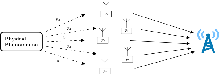
Fig. 1: System model with common alarm and standard messages. pdp_{d} denotes the probability of detecting an alarm, and psp_{s} is the probability of sending a standard message.

In this we build upon the model in [1] with an important extension: we bring in the correlation of activation and message content across different devices. This is different from the mainstream view on massive random access, where the device activation and message content is independent across the devices. An exemplary case is as follows: IoT devices can send standard messages or alarm messages, the latter with critical reliability requirement and triggered by a commonly observed phenomenon. In normal operation, standard uncorrelated messages are sent. Upon the alarm activation, a number of IoT devices will prioritize it and send the same message. This reflects the extreme all-or-nothing correlation where devices are either mutually independent, or they are completely correlated both in source information and in time. Our model intends to capture the following intuitive observation. If the number of devices that transmit the same alarm message increases, then the reliability of the alarm message increases at the expense of the decrease of the total amount of information that comes from the total population of connected IoT devices. The model can be seen as having an (alarm) event that needs to be communicated through a random subset of devices, see Fig. 1. By removing the alarm event the model boils down to the model in [1].

Differently from previous works, the per-device probability of error is not meaningful for devices transmitting the alarm event in our model. Instead, the common alarm itself can be seen as a “ghost” device, which communicates through the actual IoT devices (see Fig. 1) and we calculate the error probability with respect to this ghost device. In addition, the fact that we consider two message types (standard and alarm messages) necessitates the introduction of false positive errors, namely decoding a codeword that was not transmitted. In the system model in Fig. 1, decoding an alarm message when no alarm has occurred is critical. This type of error is, typically, not considered in a common communication-theoretic setting, where an error is defined as the event in which a decoder is not decoding a codeword correctly.

The rest of the paper is organized as follows. Section II introduces the system model including the source information and time correlations. In Section III the entropy and the spectral efficiency of the correlated devices is derived. Section IV defines the alarm random access code based on the novel error model, and the error bound is derived in Section V. Finally, numerical evaluations are presented in Section VI, and concluding remarks are given in Section VII. Table I lists the notation used in this paper.

II Correlation Model

Notation
AA: Alarm event ϵa\epsilon_{\mathrm{a}}: Target probability of error for alarm messages
NN: Total number of devices ϵsa\epsilon_{\mathrm{sa}}: Target probability of error for standard messages in alarm event
KK: Number of active devices ϵfp\epsilon_{\mathrm{fp}}: Target probability of false positive
KaK_{a}: Number of devices sending an alarm message SS: Spectral efficiency
pap_{\mathrm{a}}: Alarm probability HH: Entropy
psp_{\mathrm{s}}: Standard message probability WjW_{j} Message transmitted by the jj-th device
pdp_{\mathrm{d}}: Alarm detection probability aija_{i}^{j} (lower case): (ai,…,aj)(a_{i},\ldots,a_{j}), i≤ji\leq j for scalars/vectors
ℳs\mathcal{M}_{\mathrm{s}}: Set of standard messages XijX_{i}^{j} (upper case): (Xi,…,Xj)(X_{i},\ldots,X_{j}), i≤ji\leq j for random variables/vectors
ℳa\mathcal{M}_{\mathrm{a}}: Set of alarm messages aii−1a_{i}^{i-1}: Empty tuple
nn: Blocklength ∑i=jj−1aj\sum_{i=j}^{j-1}a_{j}: 0
P′P^{\prime}: Average transmission power [𝒮]k[\mathcal{S}]^{k} Set of all kk-subsets of the set 𝒮\mathcal{S}
PP: Maximal transmission power 𝒳\mathcal{X}: ∈ℝn\in\mathbb{R}^{n} Input alphabet
ϵs\epsilon_{\mathrm{s}}: Target probability of error for standard messages without an alarm 𝒴\mathcal{Y}: ∈ℝn\in\mathbb{R}^{n} Output alphabet
TABLE I: Notation used throughout this paper.

We consider the uplink in a random access channel in which each access opportunity is a block of nn channel uses. In each block, KK out of NN devices transmit a message from one of the two disjoint message sets ℳs\mathcal{M}_{\mathrm{s}} and ℳa\mathcal{M}_{\mathrm{a}}, consisting of Ms=|ℳs|M_{\mathrm{s}}=|\mathcal{M}_{\mathrm{s}}| standard messages and Ma=|ℳa|M_{\mathrm{a}}=|\mathcal{M}_{\mathrm{a}}| alarm messages, respectively. A typical case is having a stringent reliability requirement for the alarm messages, and a high throughput and massive access requirement for the rest. As also done in [1], we assume that the number of active devices, KK, is known by the receiver.

Let P𝒀|𝑿1K:[𝒳n]K→𝒴nP_{\bm{Y}|\bm{X}_{1}^{K}}:[\mathcal{X}^{n}]^{K}\to\mathcal{Y}^{n} be a memoryless multiple access channel (MAC) satisfying permutation invariance where 𝒳,𝒴\mathcal{X},\mathcal{Y} are the input and output alphabets. That is, the distribution P𝒀|𝑿1K(⋅|𝒙1K)P_{\bm{Y}|\bm{X}_{1}^{K}}(\cdot|\bm{x}_{1}^{K}) coincides with P𝒀|𝑿1K(⋅|𝒙π⁡(1),…,𝒙π⁡(K))P_{\bm{Y}|\bm{X}_{1}^{K}}(\cdot|\bm{x}_{\pi(1)},\ldots,\bm{x}_{\pi(K)}) for any 𝒙1K∈[𝒳n]K\bm{x}_{1}^{K}\in[\mathcal{X}^{n}]^{K} and any permutation π\pi. This assumption relates to the fact that no user identification is done at the receiver, i.e. unsourced random access [11]. Therefore, all devices use the same encoder f:ℳs∪ℳa→𝒳nf:\mathcal{M}_{\mathrm{s}}\cup\mathcal{M}_{\mathrm{a}}\to\mathcal{X}^{n} and the receiver decodes according to the possibly randomized map g:𝒴n→[ℳs∪ℳa]K−Ka+1g:~\mathcal{Y}^{n}\to[\mathcal{M}_{\mathrm{s}}\cup\mathcal{M}_{\mathrm{a}}]^{K-K_{\mathrm{a}}+1}, where KaK_{\mathrm{a}} is the random number of devices that send alarm messages and [𝒮]k[\mathcal{S}]^{k} denotes the set of all kk-subsets of the set 𝒮\mathcal{S}.

We denote the message transmitted by the jj-th device as WjW_{j}. The transmitted messages are chosen according to the following model: An alarm event, AA, occurs with probability pap_{\mathrm{a}}, and there is no alarm with probability 1−pa1-p_{\mathrm{a}}. If no alarm occurs then the system acts as in [1], i.e. each device transmits a message uniformly chosen from ℳs\mathcal{M}_{\mathrm{s}} with probability psp_{\mathrm{s}}, and it is silent with probability 1−ps1-p_{\mathrm{s}}. If an alarm occurs, with probability pdp_{\mathrm{d}} a device will detect it and transmit an alarm message. Contrary to the standard messages, all devices detecting the alarm send the same message chosen uniformly from ℳa\mathcal{M}_{\mathrm{a}}. With probability 1−pd1-p_{\mathrm{d}} the device will act as if no alarm has occurred. It follows that ℙ[Wj∈ℳa]=papd\mathbb{P}[W_{j}\in\mathcal{M}_{\mathrm{a}}]=p_{\mathrm{a}}p_{\mathrm{d}} and ℙ[Wj∈ℳs]=ps−papspd\mathbb{P}[W_{j}\in\mathcal{M}_{\mathrm{s}}]=p_{\mathrm{s}}-p_{\mathrm{a}}p_{\mathrm{s}}p_{\mathrm{d}}. Notice that the probability pdp_{\mathrm{d}} in our model is the joint event of detecting an alarm and deciding to transmit a corresponding alarm message. The latter can be seen as a system design parameter and its impact to the system performance, particularly in the tradeoff between reliability and spectral efficiency, is discussed in next section.

In contrast to practical random access scenarios, we assume that the number of active devices, KK, is known by the receiver. This assumption can be justified by noting that KK could be estimated using the same procedure as in [12]. Specifically, the base station can decode the received packets under the assumption that K=0,1,…,NK=0,1,\ldots,N, and then re-generate the resulting packets and subtract them from the received signal. KK can then be determined based on the residual, which will equal the noise 𝐙\mathbf{Z}, see (12) if the correct value of KK has been determined. Furthermore, since the number of alarm messages, KaK_{\mathrm{a}}, is assumed unknown in the model, an incorrectly estimated KK will mainly affect the decoding of the non-critical standard messages.

III Spectral efficiency

In this section, we study how the presence of common alarm messages affects the information transmitted in the system. We consider the system spectral efficiency defined as S=H⁡(W1K)nS=\frac{H(W_{1}^{K})}{n}, where KK is the number of devices transmitting messages W1,…​WKW_{1},...W_{K}, HH is the joint entropy function and nn is the blocklength.

The total number of devices, NN, in the network affects the system spectral efficiency. To see this, consider the case with a high alarm detection probability pdp_{\mathrm{d}}, a low psp_{\mathrm{s}}, alarm probability pa=0.5p_{\mathrm{a}}=0.5, and suppose we receive 1010 messages, i.e. K=10K=10. If also N=10N=10, then there is a high probability that an alarm has occurred since we know that all devices transmitted and that pdp_{\mathrm{d}} is high. Moreover, in this case all devices have most likely transmitted the same message, resulting in a low spectral efficiency. On the other hand, with N=10000N=10000 devices in the network the probability that an alarm has occurred is low, being unlikely that 99909990 devices do not detect an alarm when pdp_{\mathrm{d}} is high. In this case, the messages are likely to be distinct, resulting in a high spectral efficiency.

The exact expression for the system spectral efficiency for this model is stated in Theorem 1.

Theorem 1.

For KK out of NN received messages and correlated devices as describe in Section II the system spectral efficiency, SS, is

S=1n​∑k=1KH⁡(Wk|W1k−1),S=\frac{1}{n}\sum_{k=1}^{K}H(W_{k}|W_{1}^{k-1}), (1)

where H⁡(Wk|W1k−1)H(W_{k}|W_{1}^{k-1}) is given by

H⁡(Wk|W1k−1)=(B0+B1)​∑i=1k−1(k−1i)​pa​pdi​((1−pd)​ps)k−1−i​N0−B2​(B3​log2​B3Ma+(1−B3)​log2​1−B3Ms),\displaystyle\begin{split}H(W_{k}|W_{1}^{k-1})=&~(B_{0}+B_{1})~\sum_{i=1}^{k-1}{k-1\choose i}p_{\mathrm{a}}p_{\mathrm{d}}^{i}((1-p_{\mathrm{d}})p_{\mathrm{s}})^{k-1-i}N_{0}\\ &-B_{2}\left(B_{3}\log_{2}\frac{B_{3}}{M_{\mathrm{a}}}+(1-B_{3})\log_{2}\frac{1-B_{3}}{M_{\mathrm{s}}}\right),\end{split} (2)

and

N0\displaystyle N_{0} =(pd+(1−pd)​ps)K−(k−1)​(1−pd)N−Kpa​(pd+(1−pd)​ps)K​(1−pd)N−K+(1−pa)​psK,\displaystyle=\frac{(p_{\mathrm{d}}+(1-p_{\mathrm{d}})p_{\mathrm{s}})^{K-(k-1)}(1-p_{\mathrm{d}})^{N-K}}{p_{\mathrm{a}}(p_{\mathrm{d}}+(1-p_{\mathrm{d}})p_{\mathrm{s}})^{K}(1-p_{\mathrm{d}})^{N-K}+(1-p_{\mathrm{a}})p_{\mathrm{s}}^{K}}, (3)
B0\displaystyle B_{0} =−pdpd+(1−pd)​ps​log2⁡(pdpd+(1−pd)​ps),\displaystyle=-\frac{p_{\mathrm{d}}}{p_{\mathrm{d}}+(1-p_{\mathrm{d}})p_{\mathrm{s}}}\log_{2}\left(\frac{p_{\mathrm{d}}}{p_{\mathrm{d}}+(1-p_{\mathrm{d}})p_{\mathrm{s}}}\right), (4)
B1\displaystyle B_{1} =(1−pd)​pspd+(1−pd)​ps​(log2⁡Ms−log2⁡((1−pd)​pspd+(1−pd)​ps)),\displaystyle=\frac{(1-p_{\mathrm{d}})p_{\mathrm{s}}}{p_{\mathrm{d}}+(1-p_{\mathrm{d}})p_{\mathrm{s}}}\left(\log_{2}M_{\mathrm{s}}-\log_{2}\left(\frac{(1-p_{\mathrm{d}})p_{\mathrm{s}}}{p_{\mathrm{d}}+(1-p_{\mathrm{d}})p_{\mathrm{s}}}\right)\right), (5)
B2\displaystyle B_{2} =pa​(1−pd)N−K+(k−1)​psk−1​(pd+(1−pd)​ps)K−(k−1)+(1−pa)​psKpa​(pd+(1−pd)​ps)K​(1−pd)N−K+(1−pa)​psK,\displaystyle=\frac{p_{\mathrm{a}}(1-p_{\mathrm{d}})^{N-K+(k-1)}p_{\mathrm{s}}^{k-1}(p_{\mathrm{d}}+(1-p_{\mathrm{d}})p_{\mathrm{s}})^{K-(k-1)}+(1-p_{\mathrm{a}})p_{\mathrm{s}}^{K}}{p_{\mathrm{a}}(p_{\mathrm{d}}+(1-p_{\mathrm{d}})p_{\mathrm{s}})^{K}(1-p_{\mathrm{d}})^{N-K}+(1-p_{\mathrm{a}})p_{\mathrm{s}}^{K}}, (6)
B3\displaystyle B_{3} =pa​pd​(pd+(1−pd)​ps)K−k​(1−pd)N−K+k−1​psk−1pa​(pd+(1−pd)​ps)K−k+1​(1−pd)N−K+k−1​psk−1+(1−pa)​psK.\displaystyle=\frac{p_{\mathrm{a}}p_{\mathrm{d}}(p_{\mathrm{d}}+(1-p_{\mathrm{d}})p_{\mathrm{s}})^{K-k}(1-p_{\mathrm{d}})^{N-K+k-1}p_{\mathrm{s}}^{k-1}}{p_{\mathrm{a}}(p_{\mathrm{d}}+(1-p_{\mathrm{d}})p_{\mathrm{s}})^{K-k+1}(1-p_{\mathrm{d}})^{N-K+k-1}p_{\mathrm{s}}^{k-1}+(1-p_{\mathrm{a}})p_{\mathrm{s}}^{K}}. (7)

Proof of Theorem 1 can be found in Appendix A.

For pa=0p_{\mathrm{a}}=0 or pd=0p_{\mathrm{d}}=0 (i.e. no correlation) the system spectral efficiency is the well-known Kn​log2​Ms\frac{K}{n}\log_{2}M_{\mathrm{s}} as in [1].

IV Alarm Random Access Codes

We now define a random access code that allows for reliability diversity for standard and alarm messages. This entails having different error events for the two message types. Specifically, in order to capture the characteristics of alarm messages, we introduce reliability constraints that relates to the certainty of decoding alarm messages in the event of an alarm, but also to the certainty of not decoding alarm messages when no alarms has occurred (false positives). This is different from usual analysis since we need not only consider the event of incorrectly decoding a message, but also the type of message that is decoded instead.

The error events are listed in Table II, where we have included the “No error” column to emphasize the opposite characteristics of alarm messages and standard messages. We define error events for standard messages as in [1], i.e. errors are considered per-device and the event that more than one device sends the same standard message results in an error. In contrast, no error occurs if multiple devices transmit the same alarm message. Similarly, decoding distinct alarm messages also results in an error since only one alarm is assumed to be active at a time, while decoding distinct standard messages is naturally not an error. Formally, we define the following error events: Ej≜{Wj∉g(𝒀)}∪{Wj=Wi for some i≠j}E_{j}\triangleq\{W_{j}\notin g(\bm{Y})\}\cup\{W_{j}=W_{i}\text{ for some }i\neq j\} is the event of not decoding the message from the jj-th device, Ea≜{W0∉g(𝒀)}∪{|g(𝒀)∩ℳa|>1}E_{\mathrm{a}}\triangleq\{W_{0}\notin g(\bm{Y})\}\cup\{|g(\bm{Y})\cap\mathcal{M}_{\mathrm{a}}|>1\} for W0∈ℳaW_{0}\in\mathcal{M}_{\mathrm{a}} is the event of not decoding an alarm message or decoding more than one, and Efp≜{g(𝒀)∩ℳa≠∅}E_{\mathrm{fp}}\triangleq\{g(\bm{Y})\cap\mathcal{M}_{\mathrm{a}}\neq\varnothing\} is the event of decoding any alarm message (which is an error when no alarm has occurred). This leads to the following definition of a KK-user alarm random access (ARA) code.

Classification of events
      Error       No error
No alarm - A standard message is not decoded: - A standard message is decoded:
    {ℳs∋Wj∉g(𝒀)}\{\mathcal{M}_{\mathrm{s}}\ni W_{j}\notin g(\bm{Y})\}     {ℳs∋Wj∈g(𝒀)}\{\mathcal{M}_{\mathrm{s}}\ni W_{j}\in g(\bm{Y})\}
- More than one device sends the same message: - Different messages are sent:
    {Wj=Wi for some i≠j}\{W_{j}=W_{i}\text{ for some }i\neq j\}     {Wj≠Wi∀i≠j}\{W_{j}\neq W_{i}~\forall~i\neq j\}
- At least one alarm message is decoded: - No alarm message is decoded:
    {g(𝒀)∩ℳa≠∅}\{g(\bm{Y})\cap\mathcal{M}_{\mathrm{a}}\neq\varnothing\}  (false positive)     {g(𝒀)∩ℳa=∅}\{g(\bm{Y})\cap\mathcal{M}_{\mathrm{a}}=\varnothing\} (true negative)
Alarm - The alarm message is not decoded: - The alarm message is decoded:
    {W0∉g(𝒀)}\{W_{0}\notin g(\bm{Y})\} (false negative)     {W0∈g(𝒀)}\{W_{0}\in g(\bm{Y})\} (true positive)
- More than one alarm message is decoded: - More than one device sends the same alarm message:
    {|g(𝒀)∩ℳa|>1}\{|g(\bm{Y})\cap\mathcal{M}_{\mathrm{a}}|>1\}     {Wj=Wi=W0∈ℳa for some i≠j}\{W_{j}=W_{i}=W_{0}\in\mathcal{M}_{\mathrm{a}}\text{ for some }i\neq j\}
- A standard message is not decoded:
    {ℳs∋Wj∉g(𝒀)}\{\mathcal{M}_{\mathrm{s}}\ni W_{j}\notin g(\bm{Y})\}
- Two or more device sends the same standard
message:
    {Wi=Wj∈ℳs for some i≠j}\{W_{i}=W_{j}\in\mathcal{M}_{\mathrm{s}}\text{ for some }i\neq j\}
TABLE II: Error events in the considered system. In the alarm event we denote the alarm message by W0W_{0}.
Definition 2.

An (Ms,Ma,n,ϵa,ϵs,ϵsa,ϵfp)(M_{\mathrm{s}},M_{\mathrm{a}},n,\epsilon_{\mathrm{a}},\epsilon_{\mathrm{s}},\epsilon_{\mathrm{sa}},\epsilon_{\mathrm{fp}}) alarm random access (ARA) code for the KK-user channel P𝐘|𝐗1KP_{\bm{Y}|\bm{X}_{1}^{K}} is a pair of (possibly randomized) maps, the encoder f:ℳs∪ℳa→𝒳nf:\mathcal{M}_{\mathrm{s}}\cup\mathcal{M}_{\mathrm{a}}\to\mathcal{X}^{n}, and the decoder g:𝒴n→[ℳs∪ℳa]K−Ka+1g:\mathcal{Y}^{n}\to[\mathcal{M}_{\mathrm{s}}\cup\mathcal{M}_{\mathrm{a}}]^{K-K_{\mathrm{a}}+1} satisfying

ℙ⁡[Ea|A]\displaystyle\mathbb{P}\left[E_{\mathrm{a}}|A\right] ≤ϵa,\displaystyle\leq\epsilon_{\mathrm{a}}, (8)
1K​∑j=1Kℙ⁡[Ej|¬A]\displaystyle\frac{1}{K}\sum_{j=1}^{K}\mathbb{P}\left[E_{j}|\neg A\right] ≤ϵs,\displaystyle\leq\epsilon_{\mathrm{s}}, (9)
𝔼Ka​[1K−Ka​∑j=1K−Kaℙ⁡[Ej|A]]\displaystyle\mathbb{E}_{K_{\mathrm{a}}}\left[\frac{1}{K-K_{\mathrm{a}}}\sum_{j=1}^{K-K_{\mathrm{a}}}\mathbb{P}\left[E_{j}|A\right]\right] ≤ϵsa,\displaystyle\leq\epsilon_{\mathrm{sa}}, (10)
ℙ⁡[Efp|¬A]\displaystyle\mathbb{P}\left[E_{\mathrm{fp}}|\neg A\right] ≤ϵfp,\displaystyle\leq\epsilon_{\mathrm{fp}}, (11)

where 𝐗j=f⁡(Wj)\bm{X}_{j}=f(W_{j}), W1,…,WK∈ℳsW_{1},\ldots,W_{K}\in\mathcal{M}_{\mathrm{s}} when there is no alarm and W1,…,WK−Ka∈ℳsW_{1},\ldots,W_{K-K_{\mathrm{a}}}\in\mathcal{M}_{\mathrm{s}}, WK−Ka+1=…=WK=W0∈ℳaW_{K-K_{\mathrm{a}}+1}=\ldots=W_{K}=W_{0}\in\mathcal{M}_{\mathrm{a}} in the alarm event for a random number, KaK_{\mathrm{a}}, alarm messages.

The left hand side of (8) is the probability of not decoding or resolving the alarm message in the alarm event. The left hand side of (9) is the average per-device error probability when there is no alarm, and (10) refers to the case when there is an alarm. Lastly left hand side of (11) is the probability of false positives. In a practical scenario the entities ϵa\epsilon_{\mathrm{a}}, ϵs\epsilon_{\mathrm{s}}, ϵsa\epsilon_{\mathrm{sa}} and ϵfp\epsilon_{\mathrm{fp}} can be treated as reliability requirements, in which case the achievability of an ARA code is of interest.

In the remainder of the paper we limit the analysis to the Gaussian MAC (GMAC) given by

𝒀=∑m=1K𝑿m+𝒁.\bm{Y}=\sum_{m=1}^{K}\bm{X}_{m}+\bm{Z}. (12)

where 𝒁∈ℝn\bm{Z}\in\mathbb{R}^{n} is a standard Gaussian noise vector. Additionally a maximal average transmission power, PP, is included. That is we require ‖f⁡(Wj)‖22≤n​P\left\|{f(W_{j})}\right\|^{2}_{2}\leq nP. This model is based on the assumption that the blocklength is short enough to be within the coherence time of the channel. This allows for the devices to do channel inversion and precode their signals so that they add up coherently at the receiver. This gives the possibility of a very high reliability for alarm messages.

V Random Coding Error Bound

The achievability conditions for an ARA code are presented in Theorem 3, which provides bounds for the error probabilities ϵa\epsilon_{\mathrm{a}}, ϵs\epsilon_{\mathrm{s}}, ϵsa\epsilon_{\mathrm{sa}} and ϵfp\epsilon_{\mathrm{fp}} for a given blocklenght nn, message set sizes MaM_{\mathrm{a}} and MsM_{\mathrm{s}}, average transmission power P′P^{\prime}, and maximal transmission power PP.

Theorem 3.

Fix P′<PP^{\prime}<P. There exists an (Ma,Ms,n,ϵa,ϵs,ϵsa,ϵfp)(M_{\mathrm{a}},M_{\mathrm{s}},n,\epsilon_{\mathrm{a}},\epsilon_{\mathrm{s}},\epsilon_{\mathrm{sa}},\epsilon_{\mathrm{fp}}) alarm random access code for the KK-user GMAC satisfying power-constraint PP and

ϵa\displaystyle\epsilon_{\mathrm{a}} ≤∑Ka=0KpKa​(Ka)​a​(K,Ka)+p0,\displaystyle\leq\sum_{K_{\mathrm{a}}=0}^{K}p_{K_{\mathrm{a}}}(K_{\mathrm{a}})a(K,K_{\mathrm{a}})+p_{0}, (13)
ϵs\displaystyle\epsilon_{\mathrm{s}} ≤b⁡(K)+c⁡(K)−b⁡(K)​c​(K),\displaystyle\leq b(K)+c(K)-b(K)c(K), (14)
ϵsa\displaystyle\epsilon_{\mathrm{sa}} ≤∑Ka=0KpKa​(Ka)​(1−d⁡(K,Ka)​(1−c⁡(K−Ka)))\displaystyle\leq\sum_{K_{\mathrm{a}}=0}^{K}p_{K_{\mathrm{a}}}(K_{\mathrm{a}})\left(1-d\left(K,K_{\mathrm{a}}\right)\left(1-c\left(K-K_{\mathrm{a}}\right)\right)\right) (15)
ϵfp\displaystyle\epsilon_{\mathrm{fp}} ≤b⁡(K).\displaystyle\leq b(K). (16)

Defining ϕ⁡(k,α)=12​ln⁡(1+2​k​P′​α)\phi(k,\alpha)=\frac{1}{2}\ln(1+2kP^{\prime}\alpha) and Φ⁡(k,α)=α1+2​k​P′​α\Phi(k,\alpha)=\frac{\alpha}{1+2kP^{\prime}\alpha}, then related to (13):

pKa​(k)\displaystyle p_{K_{\mathrm{a}}}(k) =(Kk)​pdk​((1−pd)​ps)K−k(pd+(1−pd)​ps)K,\displaystyle={K\choose k}\frac{p_{\mathrm{d}}^{k}\left(\left(1-p_{\mathrm{d}}\right)p_{\mathrm{s}}\right)^{K-k}}{(p_{\mathrm{d}}+(1-p_{\mathrm{d}})p_{\mathrm{s}})^{K}}, (17)
a⁡(K,Ka)\displaystyle a(K,K_{\mathrm{a}}) =min⁡(∑Ka′=0Ke−n​Ea,1),\displaystyle=\min\left(\sum_{K_{\mathrm{a}}^{\prime}=0}^{K}e^{-nE_{\mathrm{a}}},~1\right), (18)
p0\displaystyle p_{0} =ℙ[1n∑i=1nZi2>PP′],\displaystyle=\mathbb{P}\left[\frac{1}{n}\sum_{i=1}^{n}Z_{i}^{2}>\frac{P}{P^{\prime}}\right], (19)
Ea\displaystyle E_{\mathrm{a}} =max0≤ρ≤1,0<λa−ρn​ln⁡(Ma−1)+ξa,\displaystyle=\max_{0\leq\rho\leq 1,0<\lambda_{\mathrm{a}}}-\frac{\rho}{n}\ln(M_{\mathrm{a}}-1)+\xi_{\mathrm{a}}, (20)
ξa\displaystyle\xi_{\mathrm{a}} =ρ​ϕ​(Ka′2,λa)+ϕ⁡(Ka2,ρ​βa)+ϕ⁡(K−Ka,γa)+ϕ⁡(1/P′,ψa),\displaystyle=\rho\phi(K_{\mathrm{a}}^{\prime 2},\lambda_{\mathrm{a}})+\phi(K_{\mathrm{a}}^{2},\rho\beta_{\mathrm{a}})+\phi(K-K_{\mathrm{a}},\gamma_{\mathrm{a}})+\phi(1/P^{\prime},\psi_{\mathrm{a}}), (21)
ψa\displaystyle\psi_{\mathrm{a}} =Φ⁡(K−Ka,γa),γa=Φ⁡(Ka2,ρ​βa)−ρ​λa,βa=Φ⁡(Ka′2,λa).\displaystyle=\Phi(K-K_{\mathrm{a}},\gamma_{\mathrm{a}}),~~\gamma_{\mathrm{a}}=\Phi(K_{\mathrm{a}}^{2},\rho\beta_{\mathrm{a}})-\rho\lambda_{\mathrm{a}},~~\beta_{\mathrm{a}}=\Phi(K_{\mathrm{a}}^{\prime 2},\lambda_{\mathrm{a}}). (22)

Related to (16):

b⁡(K)\displaystyle b(K) =min⁡(∑Ka′=1Ke−n​Efp,1),\displaystyle=\min\left(\sum_{K_{\mathrm{a}}^{\prime}=1}^{K}e^{-nE_{\mathrm{fp}}},~1\right), (23)
Efp\displaystyle E_{\mathrm{fp}} =max0≤ρ≤1,0<λfp−ρn​ln⁡(Ma)+ξfp,\displaystyle=\max_{0\leq\rho\leq 1,~0<\lambda_{\mathrm{fp}}}-\frac{\rho}{n}\ln(M_{\mathrm{a}})+\xi_{\mathrm{fp}}, (24)
ξfp\displaystyle\xi_{\mathrm{fp}} =ρ​ϕ​(Ka′2,λfp)+ϕ⁡(K,ρ​βfp)+ϕ⁡(1/P′,γfp),\displaystyle=\rho\phi(K_{\mathrm{a}}^{\prime 2},\lambda_{\mathrm{fp}})+\phi(K,\rho\beta_{\mathrm{fp}})+\phi(1/P^{\prime},\gamma_{\mathrm{fp}}), (25)
γfp\displaystyle\gamma_{\mathrm{fp}} =Φ⁡(K,ρ​βfp),βfp=Φ⁡(Ka′2,λfp)−λfp,\displaystyle=\Phi(K,\rho\beta_{\mathrm{fp}}),~~\beta_{\mathrm{fp}}=\Phi(K_{\mathrm{a}}^{\prime 2},\lambda_{\mathrm{fp}})-\lambda_{\mathrm{fp}}, (26)

Related to (14)

c⁡(K)\displaystyle c(K) =∑t=1KtK​min⁡(pt,qt)+(K2)Ms+K​p0,\displaystyle=\sum_{t=1}^{K}\frac{t}{K}\min(p_{t},q_{t})+\frac{{K\choose 2}}{M_{\mathrm{s}}}+Kp_{0}, (27)
pt\displaystyle p_{t} =e−n​Et,\displaystyle=e^{-nE_{t}}, (28)
Et\displaystyle E_{t} =max0≤ρ,ρ1≤1−ρ​ρ1​t​R1−ρ1​R2+E0​(ρ,ρ1),\displaystyle=\max_{0\leq\rho,\rho_{1}\leq 1}-\rho\rho_{1}tR_{1}-\rho_{1}R_{2}+E_{0}(\rho,\rho_{1}), (29)
E0​(ρ,ρ1)\displaystyle E_{0}(\rho,\rho_{1}) =ρ​ρ1​ϕ​(t,λs)+ρ1​ϕ​(t,μ)+12​ln⁡(1−2​b​ρ1),\displaystyle=\rho\rho_{1}\phi(t,\lambda_{\mathrm{s}})+\rho_{1}\phi(t,\mu)+\frac{1}{2}\ln(1-2b\rho_{1}), (30)
b\displaystyle b =ρ​λs−Φ⁡(t,μ),μ=ρ​Φ​(t,λs),λs=P′​t−1+D4​(1+ρ1​ρ)​P′​t,\displaystyle=\rho\lambda_{\mathrm{s}}-\Phi(t,\mu),~~\mu=\rho\Phi(t,\lambda_{\mathrm{s}}),~~\lambda_{\mathrm{s}}=\frac{P^{\prime}t-1+\sqrt{D}}{4(1+\rho_{1}\rho)P^{\prime}t}, (31)
D\displaystyle D =(P′​t−1)2+4​P′​t​1+ρ​ρ11+ρ,\displaystyle=(P^{\prime}t-1)^{2}+4P^{\prime}t\frac{1+\rho\rho_{1}}{1+\rho}, (32)
R1\displaystyle R_{1} =1n​ln⁡(Ms)−1n​t​ln⁡(t!),R2=1n​ln⁡(Kt),\displaystyle=\frac{1}{n}\ln(M_{s})-\frac{1}{nt}\ln(t!),~~R_{2}=\frac{1}{n}\ln{K\choose t}, (33)
qt\displaystyle q_{t} =infγsℙ[It≤γs]+en⁡(t​R1+R2)−γs,\displaystyle=\inf_{\gamma_{\mathrm{s}}}\mathbb{P}\left[I_{t}\leq\gamma_{\mathrm{s}}\right]+e^{n(tR_{1}+R_{2})-\gamma_{\mathrm{s}}}, (34)
It\displaystyle I_{t} OPEN=minS0∈[ℳs]t⁡it​(∑W∈S0𝒄W;𝒀|∑W∈S0c𝒄W)),\displaystyle=\min_{S_{0}\in[\mathcal{M}_{\mathrm{s}}]^{t}}i_{t}\left(\sum_{W\in S_{0}}\bm{c}_{W};\bm{Y}|\sum_{W\in S_{0}^{c}}\bm{c}_{W})\right), (35)
it​(𝒂;𝒚|𝒃)\displaystyle i_{t}(\bm{a};\bm{y}|\bm{b}) =n​Ct+ln⁡e2​(‖𝒚−𝒃‖221+P′​t−‖𝒚−𝒂−𝒃‖22),\displaystyle=nC_{t}+\frac{\ln e}{2}\left(\frac{\left\|{\bm{y}-\bm{b}}\right\|^{2}_{2}}{1+P^{\prime}t}-\left\|{\bm{y}-\bm{a}-\bm{b}}\right\|^{2}_{2}\right), (36)

where Ct=ϕ⁡(1/2,t)C_{t}=\phi(1/2,t), S0∈[ℳs]tS_{0}\in[\mathcal{M}_{\mathrm{s}}]^{t} is a tt-subset of true standard messages and 𝐜W∼𝒩⁡(𝟎,𝐈n​P′)\bm{c}_{W}\sim\mathcal{N}(\bm{0},\bm{I}_{n}P^{\prime}) is codeword corresponding to message WW. Related to (15):

d⁡(K,Ka)\displaystyle d(K,K_{\mathrm{a}}) =(1−(a⁡(K,Ka)+p0))​(1−e⁡(K,Ka)+p0),\displaystyle=(1-(a(K,K_{\mathrm{a}})+p_{0}))(1-e(K,K_{\mathrm{a}})+p_{0}), (37)
e⁡(K,Ka)\displaystyle e(K,K_{\mathrm{a}}) =min⁡(∑Ka′=0Ka′≠KaKe−n​Esa,1),\displaystyle=\min\left(\sum_{\begin{subarray}{c}K_{\mathrm{a}}^{\prime}=0\\ K_{\mathrm{a}}^{\prime}\neq K_{\mathrm{a}}\end{subarray}}^{K}e^{-nE_{\mathrm{sa}}},~1\right), (38)
Esa\displaystyle E_{\mathrm{sa}} =max0<λsa⁡ϕ⁡((Ka−Ka′)2,λsa)+ϕ⁡(K−Ka,βsa)+ϕ⁡(1/P′,γsa),\displaystyle=\max_{0<\lambda_{\mathrm{sa}}}\phi((K_{\mathrm{a}}-K_{\mathrm{a}}^{\prime})^{2},\lambda_{\mathrm{sa}})+\phi(K-K_{\mathrm{a}},\beta_{\mathrm{sa}})+\phi(1/P^{\prime},\gamma_{\mathrm{sa}}), (39)
γsa\displaystyle\gamma_{\mathrm{sa}} =Φ⁡(K−Ka,βsa),βsa=Φ⁡((Ka−Ka′)2,λsa)−λsa.\displaystyle=\Phi\left(K-K_{\mathrm{a}},\beta_{\mathrm{sa}}\right),\quad\beta_{\mathrm{sa}}=\Phi\left((K_{\mathrm{a}}-K_{\mathrm{a}}^{\prime})^{2},\lambda_{\mathrm{sa}}\right)-\lambda_{\mathrm{sa}}. (40)

Proof of Theorem 3 can be found in Appendix B.

VI Numerical evaluation

The bounds in Theorem 3 are given for a fixed number of active devices, KK, but the probability of a given value of KK depends on whether an alarm has happened or not. Therefore, we consider the average bound over the distribution of KK conditioned on the alarm state and the total number of devices, NN. The distribution of KK given an alarm is

pK​(k|A)=(Nk)​(pd+(1−pd)​ps)k​(1−pd)N−k​(1−ps)N−k,p_{K}(k|A)={N\choose k}(p_{\mathrm{d}}+(1-p_{\mathrm{d}})p_{\mathrm{s}})^{k}(1-p_{\mathrm{d}})^{N-k}(1-p_{\mathrm{s}})^{N-k}, (41)

and the distribution of KK given no alarm is

pK​(k|¬A)=(Nk)​psk​(1−ps)N−k.p_{K}(k|\neg A)={N\choose k}p_{\mathrm{s}}^{k}(1-p_{\mathrm{s}})^{N-k}. (42)

We first study the trade-off between the probability of error for alarm messages and the per-device spectral efficiency SS, during the event of an alarm. We consider a setting with N=1000N=$1000$ devices and a blocklength of n=30 000n=$30\,000$. The alarm and standard messages are 33 and 100100 bits, respectively. The probability of activation when there is no alarm is ps=0.01p_{\mathrm{s}}=0.01, and the transmission power is chosen such that the target average error bound for standard messages is ϵs=​10−1\epsilon_{\mathrm{s}}=${10}^{-1}$, and the probability of false positive alarms is below ϵfp=​10−5\epsilon_{\mathrm{fp}}=${10}^{-5}$. Having only a few bits for alarm messages is a realistic setting, e.g. in a sensor network the alarm could be that a sensed value is too high or too low resulting in only one bit needed for the alarm message.

Refer to caption
Fig. 2: Trade-off between probability of error for alarm messages and the spectral efficiency. Blocklength n=30 000n=$30\,000$, N=1000N=$1000$, target error probabilities ϵs=​10−1\epsilon_{\mathrm{s}}=${10}^{-1}$, ϵfp=​10−5\epsilon_{\mathrm{fp}}=${10}^{-5}$, set sizes Ms=2100M_{\mathrm{s}}=2^{100}, Ma=23M_{\mathrm{a}}=2^{3}, ps=0.01p_{\mathrm{s}}=0.01 and pa=1p_{\mathrm{a}}=1.

In Fig. 2 it can be seen that the probability of error increases for increasing spectral efficiency (decreasing pdp_{\mathrm{d}}). Notice that the maximum spectral efficiency is achieved when the error probability is one (or equivalently, pd=0p_{\mathrm{d}}=0), i.e. no alarm messages are detected. This is expected since a higher number of devices transmitting alarm messages reduces the per-device spectral efficiency, but increases the received signal-to-noise ratio of alarm messages. Furthermore, very high reliability is achievable. This trade-off between spectral efficiency and probability of error is not surprising since this is also the case when the blocklength or message set size are changed. The novelty is in the fact that it is the correlation between devices that causes the trade-off.

We now consider the minimal average transmission power, P′P^{\prime}, required to satisfy some target error probabilities. We assume no power restriction. That is p0=0p_{0}=0 in Theorem 3. Let all parameters be fixed except P′P^{\prime} and pdp_{\mathrm{d}}. This is an optimization problem on the form

minimize0≤P′,0≤pd≤1P′s.t.∑K=0NpK​(K|¬A)​(b⁡(K)+c⁡(K)−b⁡(K)​c​(K))≤ϵs∑K=0NpK​(K|¬A)​b​(K)≤ϵfp∑K=0NpK​(K|A)​∑Ka=0KpKa​(Ka)​a​(K,Ka)≤ϵa∑K=0NpK​(K|A)​∑Ka=0KpKa​(Ka)​(1−d⁡(K,Ka)​(1−c⁡(K−Ka)))≤ϵsa\begin{array}[]{lll}\displaystyle\minimize_{0\leq P^{\prime},~0\leq p_{\mathrm{d}}\leq 1}&P^{\prime}&\\ \mbox{s.t.}&\sum_{K=0}^{N}p_{K}(K|\neg A)(b(K)+c(K)-b(K)c(K))&\leq\epsilon_{\mathrm{s}}\\ &\sum_{K=0}^{N}p_{K}(K|\neg A)b(K)&\leq\epsilon_{\mathrm{fp}}\\ &\sum_{K=0}^{N}p_{K}(K|A)\sum_{K_{\mathrm{a}}=0}^{K}p_{K_{\mathrm{a}}}(K_{\mathrm{a}})a(K,K_{\mathrm{a}})&\leq\epsilon_{\mathrm{a}}\\ &\sum_{K=0}^{N}p_{K}(K|A)\sum_{K_{\mathrm{a}}=0}^{K}p_{K_{\mathrm{a}}}(K_{\mathrm{a}})(1-d(K,K_{\mathrm{a}})(1-c(K-K_{\mathrm{a}})))&\leq\epsilon_{\mathrm{sa}}\end{array} (43)

The constraint functions are strictly increasing for decreasing values of P′P^{\prime} and pdp_{\mathrm{d}}, and the first two constraints do not depend on pdp_{\mathrm{d}}. Therefore, the problem can be efficiently solved using bisection by first minimizing P′P^{\prime} subject to the first two constraints, and then determine pdp_{\mathrm{d}} from the last two constraints using the P′P^{\prime} from the previous step. This provides a feasible solution for the values of N,ϵaN,\epsilon_{\mathrm{a}} and ϵsa\epsilon_{\mathrm{sa}} of interest in this paper. However, if no feasible pd∈[0,1]p_{\mathrm{d}}\in[0,1] can be obtained from the second step, then a solution can be found by setting pd=1p_{\mathrm{d}}=1 and minimizing P′P^{\prime} subject to the last two constraints.

We use the same system parameters as in the previous scenario, except that we now fix ϵa=ϵfp=​10−5\epsilon_{\mathrm{a}}=\epsilon_{\mathrm{fp}}=${10}^{-5}$ and ϵs=ϵsa=​10−1\epsilon_{\mathrm{s}}=\epsilon_{\mathrm{sa}}=${10}^{-1}$. Based on the optimal pdp_{\mathrm{d}} and the values of psp_{\mathrm{s}}, pap_{\mathrm{a}}, we evaluate the minimal average energy-per-bit 𝔼pK​[E0N0]=n​P′2​𝔼pK​[H⁡(W1K)/K]\mathbb{E}_{p_{K}}\left[\frac{E_{0}}{N_{0}}\right]=\frac{nP^{\prime}}{2\mathbb{E}_{p_{K}}\left[H(W_{1}^{K})/K\right]}.

In Fig. 3 the solid blue line shows the energy-per-bit as a function of total number devices, NN, for this setup. Notice that optimization is done for each NN. Additionally, the achievable energy-per-bit for the uncorrelated case (pd=0)(p_{\mathrm{d}}=0) is included for reference, and is obtained as described in [1] but without the transmission power restriction. It can be seen that almost the same energy-per-bit is achievable for correlated and uncorrelated devices up to approximately 1300013000 devices, where the energy-per-bit required in the correlated case starts to increase significantly. This is due to the fact that the bound for false positives starts to dominate the choice of P′P^{\prime}. Thus, due to high multi-access interference, the probability of decoding a false positive is higher than the probability of failing to decode a standard message. The increase in power needed to accommodate the false positive target probability ϵfp\epsilon_{\mathrm{fp}} causes the error probability of standard messages to go well below their target error probability ϵs\epsilon_{\mathrm{s}}. In fact, with more than 1750017500 devices the error bound for standard messages is also approximately ​10−5{10}^{-5}. This is similar to the behavior in the uncorrelated case where the finite blocklength penalty is the dominating constraint when NN is small, while multi-access interference dominates for large NN [1]. This is seen in the increase in the slope at around 1500015000 devices in the uncorrelated case.

The effect of increasing alarm probability, pap_{\mathrm{a}}, can be seen as the dashed curves in Fig. 3. The energy-per-bit is higher for larger pap_{\mathrm{a}} due to the increased rate of alarm events where spectral efficiency is lower. The energy-per-bit in alarm events corresponds to the curve for pa=1p_{a}=1. Notice that the energy requirement P′P^{\prime} and the probability pdp_{\mathrm{d}} are not altered by varying pap_{\mathrm{a}} since the error probabilities for ARA codes are conditioned on the occurrence of an alarm. The high energy-per-bit for small NN and high pap_{\mathrm{a}} is due to the large number of devices (relative to NN) that must devote their resources to a single alarm message in order to accommodate the target alarm reliability. In general, the curves corresponding to different values of pap_{\mathrm{a}} are approaching each other for increasing NN. This is caused by the almost constant number of alarm messages required to achieve the alarm target reliability. For increasing NN this ratio of alarm messages to standard messages grows and the traffic will be mostly standard messages.

Refer to caption
Fig. 3: Trade-off between EbN0\frac{E_{b}}{N_{0}} and the number of devices, NN, for different values of alarm probability pap_{\mathrm{a}} and for uncorrelated devices. Blocklength n=30 000n=$30\,000$, target error probabilities ϵa=ϵfp=​10−5\epsilon_{\mathrm{a}}=\epsilon_{\mathrm{fp}}=${10}^{-5}$, ϵs=ϵsa=​10−1\epsilon_{\mathrm{s}}=\epsilon_{\mathrm{sa}}=${10}^{-1}$, set sizes Ms=2100M_{\mathrm{s}}=2^{100}, Ma=23M_{\mathrm{a}}=2^{3} and ps=0.01p_{\mathrm{s}}=0.01.

VII Conclusions

We have studied the trade-off between reliability and spectral efficiency in a massive random access scenario where the devices can send standard messages or alarm messages. The alarm messages are triggered by a common physical phenomenon and introduce correlation in both the transmitted messages and the activation of devices. We derive the system spectral efficiency and propose an achievability bound for alarm random access codes. We show that very reliable transmissions of alarm messages can be achieved, but that the correlation causes a trade-off in spectral efficiency. In particular, when the multi-access interference is moderate, the cost of providing high reliability of alarm messages is small in terms of the average energy-per-bit. However, when multi-access interference is high, the probability of decoding a false positive alarm message dominates the error probabilities, and the cost of providing high reliability is significant.

Appendix A Proof of Theorem 1

To explicitly show the dependency on the number of messages define

TKN={W1∈ℳa∪ℳs}∪⋯∪{WK∈ℳa∪ℳs}∪{WK+1∈∅}∪⋯∪{WN∈∅}T_{K}^{N}=\{W_{1}\in\mathcal{M}_{\mathrm{a}}\cup\mathcal{M}_{\mathrm{s}}\}\cup\cdots\cup\{W_{K}\in\mathcal{M}_{\mathrm{a}}\cup\mathcal{M}_{\mathrm{s}}\}\cup\{W_{K+1}\in\varnothing\}\cup\cdots\cup\{W_{N}\in\varnothing\} (44)

as the event that the first KK out of NN devices transmit and the rest are silent. Due to symmetry in the devices, and without loss of generality, we assume the KK first devices that are transmitting. By the law of total probability this event has probability

p⁡(TKN)=pa​(pd+(1−pd)​ps)K​(1−pd)N−K​(1−ps)N−K+(1−pa)​psK​(1−ps)N−K,p(T_{K}^{N})=p_{\mathrm{a}}(p_{\mathrm{d}}+(1-p_{\mathrm{d}})p_{\mathrm{s}})^{K}(1-p_{\mathrm{d}})^{N-K}(1-p_{\mathrm{s}})^{N-K}+(1-p_{\mathrm{a}})p_{\mathrm{s}}^{K}(1-p_{\mathrm{s}})^{N-K}, (45)

System spectral efficiency, SS, is defined as S=H⁡(W1K)/nS=H(W_{1}^{K})/n where the joint entropy of all KK messages can be expressed using the chain rule for entropy [13, Theo. 2.5.1] as

H⁡(W1K)=∑k=1KH⁡(Wk|W1k−1).H(W_{1}^{K})=\sum_{k=1}^{K}H(W_{k}|W_{1}^{k-1}). (46)

Thus we need to express the conditional entropy H⁡(Wk|W1k−1)H(W_{k}|W_{1}^{k-1}) given by

H(Wk|W1k−1)=∑w1∈ℳa∪ℳs⋯∑wk−1∈ℳa∪ℳsp(w1k−1|TKN)H(Wk|W1k−1=w1k−1),H(W_{k}|W_{1}^{k-1})=\sum_{w_{1}\in\mathcal{M}_{\mathrm{a}}\cup\mathcal{M}_{\mathrm{s}}}\cdots\sum_{w_{k-1}\in\mathcal{M}_{\mathrm{a}}\cup\mathcal{M}_{\mathrm{s}}}\!p(w_{1}^{k-1}|T_{K}^{N})H(W_{k}|W_{1}^{k-1}=w_{1}^{k-1}), (47)

where

H(Wk|W1k−1=w1k−1)=−∑wk∈ℳa∪ℳsp(wk|w1k−1,TKN)log2(p(wk|w1k−1,TKN)),H(W_{k}|W_{1}^{k-1}=w_{1}^{k-1})=-\sum_{w_{k}\in\mathcal{M}_{\mathrm{a}}\cup\mathcal{M}_{\mathrm{s}}}p(w_{k}|w_{1}^{k-1},T_{K}^{N})\log_{2}(p(w_{k}|w_{1}^{k-1},T_{K}^{N})), (48)

for k≤Kk\leq K.

Observe that ℳs\mathcal{M}_{\mathrm{s}} and ℳa\mathcal{M}_{\mathrm{a}} are disjoint so that we can split each sum in (47) into two sums over wi∈ℳaw_{i}\in\mathcal{M}_{\mathrm{a}} and wi∈ℳsw_{i}\in\mathcal{M}_{\mathrm{s}}. For convenience, we define the set Ak={w1k|w1k∈[ℳa∪ℳs]k,∃0≤i≤k:wi∈ℳa}A^{k}=\{w_{1}^{k}~|~w_{1}^{k}\in[\mathcal{M}_{\mathrm{a}}\cup\mathcal{M}_{\mathrm{s}}]^{k},\exists~0\leq i\leq k:w_{i}\in\mathcal{M}_{\mathrm{a}}\} as the set of kk-subsets of ℳa∪ℳs\mathcal{M}_{\mathrm{a}}\cup\mathcal{M}_{\mathrm{s}} that contain at least one alarm message and rewrite (47) as

H⁡(Wk|W1k−1)=∑w1k−1∈Ak−1pA​(w1k−1|TKN)​HA​(Wk|W1k−1=w1k−1)+∑w1k−1∈[ℳs]k−1pS​(w1k−1|TKN)​HS​(Wk|W1k−1=w1k−1).H(W_{k}|W_{1}^{k-1})=\sum_{w_{1}^{k-1}\in A^{k-1}}p_{\mathrm{A}}(w_{1}^{k-1}|T_{K}^{N})H_{\mathrm{A}}(W_{k}|W_{1}^{k-1}=w_{1}^{k-1})+\sum_{w_{1}^{k-1}\in[\mathcal{M}_{\mathrm{s}}]^{k-1}}p_{\mathrm{S}}(w_{1}^{k-1}|T_{K}^{N})H_{\mathrm{S}}(W_{k}|W_{1}^{k-1}=w_{1}^{k-1}). (49)

We first derive an expression for HA​(Wk|W1k−1=w1k−1)H_{\mathrm{A}}(W_{k}|W_{1}^{k-1}=w_{1}^{k-1}) using the fact that at least one of w1,…,wk−1w_{1},\ldots,w_{k-1} belongs to ℳa\mathcal{M}_{\mathrm{a}}. We additionally split the sum in (48) into two sums; one over wk∈ℳaw_{k}\in\mathcal{M}_{\mathrm{a}} and one over wk∈ℳsw_{k}\in\mathcal{M}_{\mathrm{s}}:

HA​(Wk|W1k−1=w1k−1)=−∑wk∈ℳap(wk|w1k−1∈Ak−1,TKN)log2(p(wk|w1k−1∈Ak−1,TKN))−∑wk∈ℳsp(wk|w1k−1∈Ak−1,TKN)log2(p(wk|w1k−1∈Ak−1,TKN)).\displaystyle\begin{split}H_{\mathrm{A}}(W_{k}|W_{1}^{k-1}=w_{1}^{k-1})&=-\sum_{w_{k}\in\mathcal{M}_{\mathrm{a}}}p(w_{k}|w_{1}^{k-1}\in A^{k-1},T_{K}^{N})\log_{2}(p(w_{k}|w_{1}^{k-1}\in A^{k-1},T_{K}^{N}))\\ &\quad-\sum_{w_{k}\in\mathcal{M}_{\mathrm{s}}}p(w_{k}|w_{1}^{k-1}\in A^{k-1},T_{K}^{N})\log_{2}(p(w_{k}|w_{1}^{k-1}\in A^{k-1},T_{K}^{N})).\end{split} (50)

Using Bayes’ theorem we obtain

p⁡(Wk∈ℳa|w1k−1∈Ak−1,TKN)\displaystyle p(W_{k}\in\mathcal{M}_{\mathrm{a}}|w_{1}^{k-1}\in A^{k-1},T_{K}^{N}) =p⁡(TKN|Wk∈ℳa,w1k−1∈Ak−1)​p​(Wk∈ℳa|w1k−1∈Ak−1)p⁡(TKN|w1k−1∈Ak−1)\displaystyle=\frac{p(T_{K}^{N}|W_{k}\in\mathcal{M}_{\mathrm{a}},w_{1}^{k-1}\in A^{k-1})p(W_{k}\in\mathcal{M}_{\mathrm{a}}|w_{1}^{k-1}\in A^{k-1})}{p(T_{K}^{N}|w_{1}^{k-1}\in A^{k-1})}
=(pd+(1−pd)​ps)K−k​(1−pd)N−k​(1−ps)N−k​pd(pd+(1−pd)​ps)K−(k−1)​(1−ps)N−k​(1−ps)N−k\displaystyle=\frac{(p_{\mathrm{d}}+(1-p_{\mathrm{d}})p_{\mathrm{s}})^{K-k}(1-p_{\mathrm{d}})^{N-k}(1-p_{\mathrm{s}})^{N-k}p_{\mathrm{d}}}{(p_{\mathrm{d}}+(1-p_{\mathrm{d}})p_{\mathrm{s}})^{K-(k-1)}(1-p_{\mathrm{s}})^{N-k}(1-p_{\mathrm{s}})^{N-k}}
=pdpd+(1−pd)​ps.\displaystyle=\frac{p_{\mathrm{d}}}{p_{\mathrm{d}}+(1-p_{\mathrm{d}})p_{\mathrm{s}}}. (51)

Since all devices that detect the alarm transmit the same message, the first term in (50) is

−∑wk∈ℳap(wk|w1k−1∈Ak−1,TKN)log2(p(wk|w1k−1∈Ak−1,TKN))\displaystyle-\sum_{w_{k}\in\mathcal{M}_{\mathrm{a}}}p(w_{k}|w_{1}^{k-1}\in A^{k-1},T_{K}^{N})\log_{2}(p(w_{k}|w_{1}^{k-1}\in A^{k-1},T_{K}^{N})) =−pdpd+(1−pd)​ps​log2⁡(pdpd+(1−pd)​ps)\displaystyle=-\frac{p_{\mathrm{d}}}{p_{\mathrm{d}}+(1-p_{\mathrm{d}})p_{\mathrm{s}}}\log_{2}\left(\frac{p_{\mathrm{d}}}{p_{\mathrm{d}}+(1-p_{\mathrm{d}})p_{\mathrm{s}}}\right)
≜B0.\displaystyle\triangleq B_{0}. (52)

Similarly, for the summation over wk∈ℳsw_{k}\in\mathcal{M}_{\mathrm{s}} in (50) we obtain

p⁡(Wk∈ℳs|w1k−1∈Ak−1,TKN)=(1−pd)​pspd+(1−pd)​ps=1−p⁡(Wk∈ℳa|w1k−1∈Ak−1,TKN).p(W_{k}\in\mathcal{M}_{\mathrm{s}}|w_{1}^{k-1}\in A^{k-1},T_{K}^{N})=\frac{(1-p_{\mathrm{d}})p_{\mathrm{s}}}{p_{\mathrm{d}}+(1-p_{\mathrm{d}})p_{\mathrm{s}}}=1-p(W_{k}\in\mathcal{M}_{\mathrm{a}}|w_{1}^{k-1}\in A^{k-1},T_{K}^{N}). (53)

Since the standard messages are not mutually exclusive, and equally likely, it follows that the second term in (50) becomes

−∑wk∈ℳsp(wk|w1k−1,TKN)log2(p(wk|w1k−1,TKN))=−∑wk∈ℳs1Ms(1−pd)​pspd+(1−pd)​pslog2(1Ms(1−pd)​pspd+(1−pd)​ps)=(1−pd)​pspd+(1−pd)​ps​(log2⁡Ms−log2⁡((1−pd)​pspd+(1−pd)​ps))≜B1,\displaystyle\begin{split}-\sum_{w_{k}\in\mathcal{M}_{\mathrm{s}}}p(w_{k}|w_{1}^{k-1},T_{K}^{N})\log_{2}(p(w_{k}|w_{1}^{k-1},T_{K}^{N}))&=-\sum_{w_{k}\in\mathcal{M}_{\mathrm{s}}}\frac{1}{M_{\mathrm{s}}}\frac{(1-p_{\mathrm{d}})p_{\mathrm{s}}}{p_{\mathrm{d}}+(1-p_{\mathrm{d}})p_{\mathrm{s}}}\log_{2}\left(\frac{1}{M_{\mathrm{s}}}\frac{(1-p_{\mathrm{d}})p_{\mathrm{s}}}{p_{\mathrm{d}}+(1-p_{\mathrm{d}})p_{\mathrm{s}}}\right)\\ &=\frac{(1-p_{\mathrm{d}})p_{\mathrm{s}}}{p_{\mathrm{d}}+(1-p_{\mathrm{d}})p_{\mathrm{s}}}\left(\log_{2}M_{\mathrm{s}}-\log_{2}\left(\frac{(1-p_{\mathrm{d}})p_{\mathrm{s}}}{p_{\mathrm{d}}+(1-p_{\mathrm{d}})p_{\mathrm{s}}}\right)\right)\\ &\triangleq B_{1},\end{split} (54)

Substituting (52) and (54) into (50) yields HA​(Wk|W1k−1=w1k−1)=B0+B1H_{\mathrm{A}}(W_{k}|W_{1}^{k-1}=w_{1}^{k-1})=B_{0}+B_{1}.

We now derive an expression for pA​(w1k−1|TKN)p_{\mathrm{A}}(w_{1}^{k-1}|T_{K}^{N}) in (49). Let 1≤i≤k−11\leq i\leq k-1 denote the (random) number of alarm messages in w1k−1w_{1}^{k-1} and, without loss of generality, assume that the alarm messages occupy the first ii positions of W1k−1W_{1}^{k-1}, i.e. w1,…,wi∈[ℳa]iw_{1},\ldots,w_{i}\in[\mathcal{M}_{\mathrm{a}}]^{i} and wi+1,…,wk−1∈[ℳs]k−i+1w_{i+1},\ldots,w_{k-1}\in[\mathcal{M}_{\mathrm{s}}]^{k-i+1}. For a fixed ii, the probability pA​(w1k−1|TKN)p_{\mathrm{A}}(w_{1}^{k-1}|T_{K}^{N}) is obtained using Bayes’ theorem as

pA(W1i=w1i∈[ℳa]i,Wi+1k−1=wi+1k−1∈[ℳs]k−(i+1)|TKN)\displaystyle p_{\mathrm{A}}(W_{1}^{i}=w_{1}^{i}\in[\mathcal{M}_{\mathrm{a}}]^{i},W_{i+1}^{k-1}=w_{i+1}^{k-1}\in[\mathcal{M}_{\mathrm{s}}]^{k-(i+1)}|T_{K}^{N})
=1Ma​Msk−(i+1)​(pd+(1−pd)​ps)K−(k−1)​(1−pd)N−K​pa​pdi​(1−pd)k−(i+1)​psk−(i+1)pa​(pd+(1−pd)​ps)K​(1−pd)N−K+(1−pa)​psK\displaystyle=\frac{1}{M_{\mathrm{a}}M_{\mathrm{s}}^{k-(i+1)}}\frac{(p_{\mathrm{d}}+(1-p_{\mathrm{d}})p_{\mathrm{s}})^{K-(k-1)}(1-p_{\mathrm{d}})^{N-K}p_{\mathrm{a}}p_{\mathrm{d}}^{i}(1-p_{\mathrm{d}})^{k-(i+1)}p_{\mathrm{s}}^{k-(i+1)}}{p_{\mathrm{a}}(p_{\mathrm{d}}+(1-p_{\mathrm{d}})p_{\mathrm{s}})^{K}(1-p_{\mathrm{d}})^{N-K}+(1-p_{\mathrm{a}})p_{\mathrm{s}}^{K}}
=pa​pdi​((1−pd)​ps)k−1−iMa​Msk−1−i​N0\displaystyle=\frac{p_{\mathrm{a}}p_{\mathrm{d}}^{i}((1-p_{\mathrm{d}})p_{\mathrm{s}})^{k-1-i}}{M_{\mathrm{a}}M_{\mathrm{s}}^{k-1-i}}N_{0} (55)

where N0N_{0} is given as in (3). Notice that as before only one alarm message is used at a given time so MaM_{\mathrm{a}} is not raised to the power of ii. Since there are exactly (k−1i)​Ma​Msk−1−i{k-1\choose i}M_{\mathrm{a}}M_{\mathrm{s}}^{k-1-i} equiprobable and disjoint message sets w1k−1w_{1}^{k-1} consisting of ii alarm messages and k−1−ik-1-i standard messages, the first term of (49) can be expressed as

∑w1k−1∈Ak−1pA​(w1k−1|TKN)​HA​(Wk|W1k−1=w1k−1)\displaystyle\sum_{w_{1}^{k-1}\in A^{k-1}}p_{\mathrm{A}}(w_{1}^{k-1}|T_{K}^{N})H_{\mathrm{A}}(W_{k}|W_{1}^{k-1}=w_{1}^{k-1}) =∑i=1k−1(k−1i)​∑w1i∈[ℳa]iwi+1k−1∈[ℳs]k−1−ipa​pdi​((1−pd)​ps)k−1−iMa​Msk−1−i​N0​(B0+B1)\displaystyle=\sum_{i=1}^{k-1}{k-1\choose i}\sum_{\begin{subarray}{c}w_{1}^{i}\in[\mathcal{M}_{\mathrm{a}}]^{i}\\ w_{i+1}^{k-1}\in[\mathcal{M}_{\mathrm{s}}]^{k-1-i}\end{subarray}}\frac{p_{\mathrm{a}}p_{\mathrm{d}}^{i}((1-p_{\mathrm{d}})p_{\mathrm{s}})^{k-1-i}}{M_{\mathrm{a}}M_{\mathrm{s}}^{k-1-i}}N_{0}(B_{0}+B_{1}) (56)
=(B0+B1)​∑i=1k−1(k−1i)​pa​pdi​((1−pd)​ps)k−1−i​N0.\displaystyle=(B_{0}+B_{1})\sum_{i=1}^{k-1}{k-1\choose i}p_{\mathrm{a}}p_{\mathrm{d}}^{i}((1-p_{\mathrm{d}})p_{\mathrm{s}})^{k-1-i}N_{0}. (57)

We now consider the second term in (49). Here the conditional messages in HSH_{\mathrm{S}} and messages in pSp_{\mathrm{S}} are all standard messages. In contrast to the previous case, this can happen both when there is no alarm, and when there is alarm but none of the devices detect it. As before, we rewrite (48) as

HS​(Wk|W1k−1=w1k−1)=−∑wk∈ℳap(wk|w1k−1∈[ℳs]k−1,TKN)log2(p(wk|w1k−1∈[ℳs]k−1,TKN))−∑wk∈ℳsp(wk|w1k−1∈[ℳs]k−1,TKN)log2(p(wk|w1k−1∈[ℳs]k−1,TKN)).\displaystyle\begin{split}H_{\mathrm{S}}(W_{k}|W_{1}^{k-1}=w_{1}^{k-1})&=-\sum_{w_{k}\in\mathcal{M}_{\mathrm{a}}}p(w_{k}|w_{1}^{k-1}\in[\mathcal{M}_{\mathrm{s}}]^{k-1},T_{K}^{N})\log_{2}(p(w_{k}|w_{1}^{k-1}\in[\mathcal{M}_{\mathrm{s}}]^{k-1},T_{K}^{N}))\\ &\quad-\sum_{w_{k}\in\mathcal{M}_{\mathrm{s}}}p(w_{k}|w_{1}^{k-1}\in[\mathcal{M}_{\mathrm{s}}]^{k-1},T_{K}^{N})\log_{2}(p(w_{k}|w_{1}^{k-1}\in[\mathcal{M}_{\mathrm{s}}]^{k-1},T_{K}^{N})).\end{split} (58)

Since each alarm message is equally likely, applying Bayes’ theorem and the law of total probability repeatedly yields

p⁡(wk∈ℳa|w1k−1∈[ℳs]k−1,TKN)\displaystyle p(w_{k}\in\mathcal{M}_{\mathrm{a}}|w_{1}^{k-1}\in[\mathcal{M}_{\mathrm{s}}]^{k-1},T_{K}^{N}) =1Ma​pa​pd​(pd+(1−pd)​ps)K−k​(1−pd)N−K+k−1​psk−1pa​(pd+(1−pd)​ps)K−k+1​(1−pd)N−K+k−1​psk−1+(1−pa)​psK\displaystyle=\frac{1}{M_{\mathrm{a}}}\frac{p_{\mathrm{a}}p_{\mathrm{d}}(p_{\mathrm{d}}+(1-p_{\mathrm{d}})p_{\mathrm{s}})^{K-k}(1-p_{\mathrm{d}})^{N-K+k-1}p_{\mathrm{s}}^{k-1}}{p_{\mathrm{a}}(p_{\mathrm{d}}+(1-p_{\mathrm{d}})p_{\mathrm{s}})^{K-k+1}(1-p_{\mathrm{d}})^{N-K+k-1}p_{\mathrm{s}}^{k-1}+(1-p_{\mathrm{a}})p_{\mathrm{s}}^{K}} (59)
≜1Ma​B3.\displaystyle\triangleq\frac{1}{M_{\mathrm{a}}}B_{3}. (60)

Similarly, for p⁡(wk∈ℳs|w1k−1∈[ℳs]k−1,TKN)p(w_{k}\in\mathcal{M}_{\mathrm{s}}|w_{1}^{k-1}\in[\mathcal{M}_{\mathrm{s}}]^{k-1},T_{K}^{N}) we obtain

p⁡(wk∈ℳs|w1k−1∈[ℳs]k−1,TKN)=1Ms​(1−B3).p(w_{k}\in\mathcal{M}_{\mathrm{s}}|w_{1}^{k-1}\in[\mathcal{M}_{\mathrm{s}}]^{k-1},T_{K}^{N})=\frac{1}{M_{\mathrm{s}}}(1-B_{3}). (61)

Therefore we get

HS​(Wk|W1k−1=w1k−1)\displaystyle H_{\mathrm{S}}(W_{k}|W_{1}^{k-1}=w_{1}^{k-1}) =−∑wk∈ℳaB3Malog2B3Ma−∑wk∈ℳs1−B3Mslog21−B3Ms\displaystyle=-\sum_{w_{k}\in\mathcal{M}_{\mathrm{a}}}\frac{B_{3}}{M_{\mathrm{a}}}\log_{2}\frac{B_{3}}{M_{\mathrm{a}}}-\sum_{w_{k}\in\mathcal{M}_{\mathrm{s}}}\frac{1-B_{3}}{M_{\mathrm{s}}}\log_{2}\frac{1-B_{3}}{M_{\mathrm{s}}} (62)
=−B3​log2​B3Ma−(1−B3)​log2​1−B3Ms.\displaystyle=-B_{3}\log_{2}\frac{B_{3}}{M_{\mathrm{a}}}-(1-B_{3})\log_{2}\frac{1-B_{3}}{M_{\mathrm{s}}}. (63)

Finally, pS​(w1k−1|TKN)p_{\mathrm{S}}(w_{1}^{k-1}|T_{K}^{N}) is given by

p⁡(w1k−1∈[ℳs]k−1|TKN)=1Msk−1​pa​(1−pd)N−K+(k−1)​psk−1​(pd+(1−pd)​ps)K−(k−1)+(1−pa)​psKpa​(pd+(1−pd)​ps)K​(1−pd)N−K+(1−pa)​psK≜1Msk−1​B2.\displaystyle\begin{split}p(w_{1}^{k-1}\in[\mathcal{M}_{\mathrm{s}}]^{k-1}|T_{K}^{N})&=\frac{1}{M_{\mathrm{s}}^{k-1}}\frac{p_{\mathrm{a}}(1-p_{\mathrm{d}})^{N-K+(k-1)}p_{\mathrm{s}}^{k-1}(p_{\mathrm{d}}+(1-p_{\mathrm{d}})p_{\mathrm{s}})^{K-(k-1)}+(1-p_{\mathrm{a}})p_{\mathrm{s}}^{K}}{p_{\mathrm{a}}(p_{\mathrm{d}}+(1-p_{\mathrm{d}})p_{\mathrm{s}})^{K}(1-p_{\mathrm{d}})^{N-K}+(1-p_{\mathrm{a}})p_{\mathrm{s}}^{K}}\\ &\triangleq\frac{1}{M_{\mathrm{s}}^{k-1}}B_{2}.\end{split} (64)

Using (63) and (64), the last term in (49) can be expressed as

∑w1k−1∈[ℳs]k−1pS​(w1k−1|TKN)​HS​(Wk|W1k−1=w1k−1)\displaystyle\sum_{w_{1}^{k-1}\in[\mathcal{M}_{\mathrm{s}}]^{k-1}}p_{\mathrm{S}}(w_{1}^{k-1}|T_{K}^{N})H_{\mathrm{S}}(W_{k}|W_{1}^{k-1}=w_{1}^{k-1}) =∑w1k−1∈[ℳs]k−1B2Msk−1​(−B3​log2​B3Ma−(1−B3)​log2​1−B3Ms)\displaystyle=\sum_{w_{1}^{k-1}\in[\mathcal{M}_{\mathrm{s}}]^{k-1}}\frac{B_{2}}{M_{\mathrm{s}}^{k-1}}\left(-B_{3}\log_{2}\frac{B_{3}}{M_{\mathrm{a}}}-(1-B_{3})\log_{2}\frac{1-B_{3}}{M_{\mathrm{s}}}\right) (65)
=−B2​(B3​log2​B3Ma+(1−B3)​log2​1−B3Ms)\displaystyle=-B_{2}\left(B_{3}\log_{2}\frac{B_{3}}{M_{\mathrm{a}}}+(1-B_{3})\log_{2}\frac{1-B_{3}}{M_{\mathrm{s}}}\right) (66)

Inserting (57) and (66) into (47) yields the final expression:

H⁡(Wk|W1k−1)=(B0+B1)​∑i=1k−1(k−1i)​pa​pdi​((1−pd)​ps)k−1−i​N0−B2​(B3​log2​B3Ma+(1−B3)​log2​1−B3Ms)H(W_{k}|W_{1}^{k-1})=(B_{0}+B_{1})\sum_{i=1}^{k-1}{k-1\choose i}p_{\mathrm{a}}p_{\mathrm{d}}^{i}((1-p_{\mathrm{d}})p_{\mathrm{s}})^{k-1-i}N_{0}-B_{2}\left(B_{3}\log_{2}\frac{B_{3}}{M_{\mathrm{a}}}+(1-B_{3})\log_{2}\frac{1-B_{3}}{M_{\mathrm{s}}}\right) (67)

∎

Appendix B Proof of Theorem 3

Generate the Ma+Ms=MM_{\mathrm{a}}+M_{\mathrm{s}}=M codewords 𝒄1,…,𝒄M∼i.i.d.𝒩⁡(𝟎,P′​𝑰n)\bm{c}_{1},\ldots,\bm{c}_{M}\stackrel{{\scriptstyle i.i.d.}}{{\sim}}\mathcal{N}(\bm{0},P^{\prime}\bm{I}_{n}). We assume that the first MaM_{\mathrm{a}} codewords are alarm messages and the last MsM_{\mathrm{s}} codewords are standards messages. Recall that WjW_{j} is the codeword selected by the jj-th device. If ‖𝒄Wj‖22>n​P\|\bm{c}_{W_{j}}\|_{2}^{2}>nP then device jj transmits 𝟎\bm{0} instead, i.e. 𝑿j=𝟎\bm{X}_{j}=\bm{0}, otherwise 𝑿j=𝒄Wj\bm{X}_{j}=\bm{c}_{W_{j}}, 1≤j≤K1\leq j\leq K. Decoding is done in two steps. The transmitted alarm message (if any) is decoded first and canceled from the received signal, and then the decoder proceeds to decoding the standard messages. Notice that the order of decoding reflects the fact that alarm messages are expected to have a higher reliability requirement than standard messages.

In the first step, the decoder estimates the transmitted alarm message W^\widehat{W} and the number of devices transmitting the alarm message K^a\widehat{K}_{\mathrm{a}}:

W^,K^a=arg​minW∈ℳa0≤Ka≤K⁡‖Ka​𝐜W−𝐘‖22.\displaystyle\widehat{W},\widehat{K}_{\mathrm{a}}=\argmin_{\begin{subarray}{c}W\in\mathcal{M}_{\mathrm{a}}\\ 0\leq K_{\mathrm{a}}\leq K\end{subarray}}\|K_{\mathrm{a}}\bm{c}_{W}-\bm{Y}\|_{2}^{2}. (68)

If K^a≥1\widehat{K}_{\mathrm{a}}\geq 1 the decoder outputs W^\widehat{W} as the alarm message and zero otherwise. The estimated interference from the alarm messages is subtracted from the received signal in a successive interference cancellation fashion as 𝒀SIC=𝒀−K^a​𝒄W^\bm{Y}_{\text{SIC}}=\bm{Y}-\widehat{K}_{\mathrm{a}}\bm{c}_{\widehat{W}}. Next the decoder outputs the set of standard messages 𝒮^∈[ℳs]K−K^a\hat{\mathcal{S}}\in[\mathcal{M}_{\mathrm{s}}]^{K-\hat{K}_{\mathrm{a}}}

𝒮^=arg​min𝒮∈[ℳs]K−K^a⁡‖∑W∈𝒮𝐜W−𝐘SIC‖22.\displaystyle\hat{\mathcal{S}}=\argmin_{\mathcal{S}\in[\mathcal{M}_{\mathrm{s}}]^{K-\hat{K}_{\mathrm{a}}}}\left\|{\sum_{W\in\mathcal{S}}\bm{c}_{W}-\bm{Y}_{\text{SIC}}}\right\|^{2}_{2}. (69)

We consider Gallager type bounds [14]. Initially we ignore the power constraint and assume that the transmitted codewords are 𝑿j=𝒄Wj\bm{X}_{j}=\bm{c}_{W_{j}} instead of 𝑿j=𝒄Wj𝟙{‖𝒄Wj‖22<nP}\bm{X}_{j}=\bm{c}_{W_{j}}\mathds{1}\{\left\|{\bm{c}_{W_{j}}}\right\|^{2}_{2}<nP\}. Furthermore, we assume that WjW_{j} are drawn without replacement from ℳs\mathcal{M}_{\mathrm{s}}. The contributions from these assumptions will be taken into account later. We consider each of the four bounds in the theorem separately.

B-A Alarm decoding error

We start with the bound in (13), i.e. the probability of not decoding an alarm message in the alarm event, denoted by ℙ⁡[Ea|A]\mathbb{P}\left[E_{\mathrm{a}}|A\right]. From symmetry we assume that devices 1,…,Ka1,\ldots,K_{\mathrm{a}} are transmitting alarm message 1=W1=W2=⋯=WKa1=W_{1}=W_{2}=\cdots=W_{K_{\mathrm{a}}}. We want to bound ℙ[W^≠1]\mathbb{P}\left[\widehat{W}\neq 1\right]. Define the interference as 𝑺=∑m=Ka+1K𝑿m\bm{S}=\sum_{m=K_{\mathrm{a}}+1}^{K}\bm{X}_{m}, where we note the dependency on KaK_{\mathrm{a}}. We then have 𝒀=Ka​𝑿1+𝑺+𝒁\bm{Y}=K_{\mathrm{a}}\bm{X}_{1}+\bm{S}+\bm{Z}. Let W′W^{\prime} be a random index in ℳa∖1\mathcal{M}_{\mathrm{a}}\setminus 1 and let 0≤Ka′≤K0\leq K_{\mathrm{a}}^{\prime}\leq K be some integer. Then by definition of the decoder (68) an error occurs if

‖Ka′​𝒄W′−(Ka​𝑿1+𝑺+𝒁)‖22<‖Ka​𝑿1−(Ka​𝑿1+𝑺+𝒁)‖22,\|K_{\mathrm{a}}^{\prime}\bm{c}_{W^{\prime}}-(K_{\mathrm{a}}\bm{X}_{1}+\bm{S}+\bm{Z})\|_{2}^{2}<\|K_{\mathrm{a}}\bm{X}_{1}-(K_{\mathrm{a}}\bm{X}_{1}+\bm{S}+\bm{Z})\|_{2}^{2}, (70)

i.e. if the distance, in L2L_{2}-norm, from a multiple of a wrong codeword 𝒄W′\bm{c}_{W^{\prime}} to the received signal 𝒀\bm{Y} is smaller than from the KaK_{\mathrm{a}} true alarm transmissions 𝑿1\bm{X}_{1}. We therefore define the error event

Fa(W′,Ka′)={∥Ka𝑿1−Ka′𝒄W′+𝑺+𝒁∥22<∥𝑺+𝒁∥22}F_{\mathrm{a}}(W^{\prime},K_{\mathrm{a}}^{\prime})=\{\|K_{\mathrm{a}}\bm{X}_{1}-K_{\mathrm{a}}^{\prime}\bm{c}_{W^{\prime}}+\bm{S}+\bm{Z}\|_{2}^{2}<\|\bm{S}+\bm{Z}\|_{2}^{2}\} (71)

We want to bound the probability of this event for all possible combinations of W′W^{\prime} and Ka′K_{\mathrm{a}}^{\prime}, thus we define the collection of events

Fa​(Ka′)=⋃W′∈ℳa∖1Fa​(W′,Ka′)F_{\mathrm{a}}(K_{\mathrm{a}}^{\prime})=\bigcup_{W^{\prime}\in{\mathcal{M}_{\mathrm{a}}\setminus 1}}F_{\mathrm{a}}(W^{\prime},K_{\mathrm{a}}^{\prime}) (72)

and

Fa=⋃0≤Ka′≤KFa​(Ka′).F_{\mathrm{a}}=\bigcup_{0\leq K_{\mathrm{a}}^{\prime}\leq K}F_{\mathrm{a}}(K_{\mathrm{a}}^{\prime}). (73)

Clearly, ℙ[Fa]=ℙ[W^≠1]=ℙ[Ea|A]\mathbb{P}\left[F_{\mathrm{a}}\right]=\mathbb{P}\left[\widehat{W}\neq 1\right]=\mathbb{P}\left[E_{\mathrm{a}}|A\right] since the decoder is designed to only output one alarm message, thereby eliminating the possibility of collision of alarm messages at the decoder.

We first use the fact that 𝑺\bm{S} is a sum of Gaussian random vectors and hence is also Gaussian, and obtain the bound

ℙ[Fa(W′,Ka′)|𝑿1,Ka,𝑺,𝒁]\displaystyle\mathbb{P}\left[F_{\mathrm{a}}(W^{\prime},K_{\mathrm{a}}^{\prime})|\bm{X}_{1},K_{\mathrm{a}},\bm{S},\bm{Z}\right] ≤eλa​‖𝑺+𝒁‖22​𝔼𝒄W′​[e−λa​‖Ka​𝑿1−Ka′​𝒄W′+𝑺+𝒁‖22]\displaystyle\leq e^{\lambda_{\mathrm{a}}\|\bm{S}+\bm{Z}\|_{2}^{2}}\mathbb{E}_{\bm{c}_{W^{\prime}}}\left[e^{-\lambda_{\mathrm{a}}\|K_{\mathrm{a}}\bm{X}_{1}-K_{\mathrm{a}}^{\prime}\bm{c}_{W^{\prime}}+\bm{S}+\bm{Z}\|_{2}^{2}}\right] (74)
=eλa​‖𝑺+𝒁‖22​e−λa​‖Ka​𝑿1+𝑺+𝒁‖221+2​Ka′2​P′​λa(1+2​Ka′2​P′​λa)n/2\displaystyle=e^{\lambda_{\mathrm{a}}\|\bm{S}+\bm{Z}\|_{2}^{2}}\frac{e^{-\frac{\lambda_{\mathrm{a}}\|K_{\mathrm{a}}\bm{X}_{1}+\bm{S}+\bm{Z}\|_{2}^{2}}{1+2K_{\mathrm{a}}^{\prime 2}P^{\prime}\lambda_{\mathrm{a}}}}}{(1+2K_{\mathrm{a}}^{\prime 2}P^{\prime}\lambda_{\mathrm{a}})^{n/2}} (75)
=eλa​‖𝑺+𝒁‖22​e−λa​‖Ka​𝑿1+𝑺+𝒁‖221+2​Ka′2​P′​λa​e−n2​ln⁡(1+2​Ka′2​P′​λa)\displaystyle=e^{\lambda_{\mathrm{a}}\|\bm{S}+\bm{Z}\|_{2}^{2}}e^{-\frac{\lambda_{\mathrm{a}}\|K_{\mathrm{a}}\bm{X}_{1}+\bm{S}+\bm{Z}\|_{2}^{2}}{1+2K_{\mathrm{a}}^{\prime 2}P^{\prime}\lambda_{\mathrm{a}}}}e^{-\frac{n}{2}\ln(1+2K_{a}^{\prime 2}P^{\prime}\lambda_{\mathrm{a}})} (76)
=eλa​‖𝑺+𝒁‖22−βa​‖Ka​𝑿1+𝑺+𝒁‖22−n​ϕ​(Ka′2,λa),\displaystyle=e^{\lambda_{\mathrm{a}}\left\|{\bm{S}+\bm{Z}}\right\|^{2}_{2}-\beta_{\mathrm{a}}\left\|{K_{a}\bm{X}_{1}+\bm{S}+\bm{Z}}\right\|^{2}_{2}-n\phi(K_{a}^{\prime 2},\lambda_{\mathrm{a}})}, (77)

where λa∈ℝ+\lambda_{\mathrm{a}}\in\mathbb{R}_{+}, ϕ⁡(k,α)=12​ln⁡(1+2​k​P′​α)\phi(k,\alpha)=\frac{1}{2}\ln(1+2kP^{\prime}\alpha) and βa=Φ⁡(Ka′2,λa)\beta_{\mathrm{a}}=\Phi(K_{a}^{\prime 2},\lambda_{\mathrm{a}}) where Φ⁡(k,α)≜α1+2​k​P′​α\Phi(k,\alpha)\triangleq\frac{\alpha}{1+2kP^{\prime}\alpha}. The bound in (74) follows from the Chernoff bound [15] and (75) uses the identity [1]

𝔼⁡[e−γ​‖α​𝑸+𝒖‖22]=e−γ​‖𝒖‖221+2​α​γ(1+2​α​γ)n/2,\mathbb{E}\left[e^{-\gamma\|\sqrt{\alpha}\bm{Q}+\bm{u}\|_{2}^{2}}\right]=\frac{e^{-\frac{\gamma\|\bm{u}\|_{2}^{2}}{1+2\alpha\gamma}}}{(1+2\alpha\gamma)^{n/2}}, (78)

where 𝒖∈ℝn\bm{u}\in\mathbb{R}^{n}, α∈ℝ+\alpha\in\mathbb{R}_{+}, γ≥−12​α\gamma\geq-\frac{1}{2\alpha} and 𝑸∼𝒩⁡(𝟎,𝑰nCLOSE\bm{Q}\sim\mathcal{N}(\bm{0},\bm{I}_{n}).

Next we use Gallager’s ρ\rho-trick [14] to bound ℙ⁡[Fa​(Ka′)]\mathbb{P}\left[F_{\mathrm{a}}(K_{\mathrm{a}}^{\prime})\right]. For events A1,A2,…A_{1},A_{2},\ldots and ρ∈[0,1]\rho\in[0,1] we have ℙ[∪jAj]≤(∑jℙ[Aj])ρ\mathbb{P}\left[\cup_{j}A_{j}\right]\leq\left(\sum_{j}\mathbb{P}\left[A_{j}\right]\right)^{\rho}. We get

ℙ[Fa(Ka′)|𝑿1,Ka,𝑺,𝒁]≤(Ma−1)ρeρ​λa​‖𝑺+𝒁‖22−ρ​βa​‖Ka​𝑿1+𝑺+𝒁‖22−ρ​n​ϕ​(Ka′2,λa).\mathbb{P}\left[F_{\mathrm{a}}(K_{\mathrm{a}}^{\prime})|\bm{X}_{1},K_{\mathrm{a}},\bm{S},\bm{Z}\right]\leq\left(M_{\mathrm{a}}-1\right)^{\rho}e^{\rho\lambda_{\mathrm{a}}\|\bm{S}+\bm{Z}\|_{2}^{2}-\rho\beta_{\mathrm{a}}\|K_{\mathrm{a}}\bm{X}_{1}+\bm{S}+\bm{Z}\|_{2}^{2}-\rho n\phi(K_{\mathrm{a}}^{\prime 2},\lambda_{\mathrm{a}})}. (79)

Taking expectation over 𝑿1\bm{X}_{1} and using (78) yields

ℙ[Fa(Ka′)|Ka,𝑺,𝒁]\displaystyle\mathbb{P}\left[F_{\mathrm{a}}(K_{\mathrm{a}}^{\prime})|K_{\mathrm{a}},\bm{S},\bm{Z}\right] ≤(Ma−1)ρ​eρ​λa​‖𝑺+𝒁‖22​𝔼𝑿1​[e−ρ​βa​‖Ka​𝑿1+𝑺+𝒁‖22]​e−ρ​n​ϕ​(Ka′2,λa)\displaystyle\leq(M_{\mathrm{a}}-1)^{\rho}e^{\rho\lambda_{\mathrm{a}}\left\|{\bm{S}+\bm{Z}}\right\|^{2}_{2}}\mathbb{E}_{\bm{X}_{1}}\left[e^{-\rho\beta_{\mathrm{a}}\left\|{K_{\mathrm{a}}\bm{X}_{1}+\bm{S}+\bm{Z}}\right\|^{2}_{2}}\right]e^{-\rho n\phi(K_{\mathrm{a}}^{\prime 2},\lambda_{\mathrm{a}})} (80)
=(Ma−1)ρ​eρ​λa​‖𝑺+𝒁‖22​e−ρ​βa​‖𝑺+𝒁‖221+2​Ka2​P′​ρ​βa(1+2​Ka2​P′​ρ​βa)n/2​e−ρ​n​ϕ​(Ka′2,λa)\displaystyle=(M_{\mathrm{a}}-1)^{\rho}e^{\rho\lambda_{\mathrm{a}}\left\|{\bm{S}+\bm{Z}}\right\|^{2}_{2}}\frac{e^{-\frac{\rho\beta_{\mathrm{a}}\left\|{\bm{S}+\bm{Z}}\right\|^{2}_{2}}{1+2K_{a}^{2}P^{\prime}\rho\beta_{\mathrm{a}}}}}{(1+2K_{a}^{2}P^{\prime}\rho\beta_{\mathrm{a}})^{n/2}}e^{-\rho n\phi(K_{a}^{\prime 2},\lambda_{\mathrm{a}})} (81)
=(Ma−1)ρ​e−γa​‖𝑺+𝒁‖22−n​τ,\displaystyle=(M_{\mathrm{a}}-1)^{\rho}e^{-\gamma_{\mathrm{a}}\|\bm{S}+\bm{Z}\|_{2}^{2}-n\tau}, (82)

where τ=ρ​ϕ​(Ka′2,λa)+ϕ⁡(Ka2,ρ​βa)\tau=\rho\phi(K_{\mathrm{a}}^{\prime 2},\lambda_{\mathrm{a}})+\phi(K_{\mathrm{a}}^{2},\rho\beta_{\mathrm{a}}) and γa=Φ⁡(Ka2,ρ​βa)−ρ​λa\gamma_{\mathrm{a}}=\Phi(K_{\mathrm{a}}^{2},\rho\beta_{\mathrm{a}})-\rho\lambda_{\mathrm{a}}. Now in the same manner as in (80)-(82) expectation is taken over 𝑺\bm{S} and 𝒁\bm{Z} where (78) is used for both. We get

ℙ⁡[Fa​(Ka′)|Ka]≤eρ​ln⁡(Ma−1)−n​ξa,\mathbb{P}\left[F_{\mathrm{a}}(K_{\mathrm{a}}^{\prime})|K_{\mathrm{a}}\right]\leq e^{\rho\ln(M_{\mathrm{a}}-1)-n\xi_{\mathrm{a}}}, (83)

where ξa=τ+ϕ⁡(K−Ka,γa)+ϕ⁡(1/P′,ψa)\xi_{\mathrm{a}}=\tau+\phi(K-K_{\mathrm{a}},\gamma_{\mathrm{a}})+\phi(1/P^{\prime},\psi_{\mathrm{a}}) and ψa=Φ⁡(K−Ka,γa)\psi_{\mathrm{a}}=\Phi(K-K_{\mathrm{a}},\gamma_{\mathrm{a}}). Introducing Ea=max0≤ρ≤1,0<λa−ρn​ln⁡(Ma−1)+ξaE_{\mathrm{a}}=\max_{0\leq\rho\leq 1,0<\lambda_{\mathrm{a}}}-\frac{\rho}{n}\ln(M_{\mathrm{a}}-1)+\xi_{\mathrm{a}} and applying the union bound gives

ℙ⁡[Fa|Ka]\displaystyle\mathbb{P}\left[F_{\mathrm{a}}|K_{\mathrm{a}}\right] =min⁡(∑Ka′=0Ke−n​Ea,1)\displaystyle=\min\left(\sum_{K_{\mathrm{a}}^{\prime}=0}^{K}e^{-nE_{\mathrm{a}}},~1\right) (84)
≜a⁡(K,Ka).\displaystyle\triangleq a(K,K_{\mathrm{a}}). (85)

Finally, we take the expectation over KaK_{\mathrm{a}}. The distribution of KaK_{\mathrm{a}} is a binomial distribution given by

pKa​(k)=(Kk)​pdk​((1−pd)​ps)K−k(pd+(1−pd)​ps)K,p_{K_{\mathrm{a}}}(k)={K\choose k}\frac{p_{\mathrm{d}}^{k}\left(\left(1-p_{\mathrm{d}}\right)p_{\mathrm{s}}\right)^{K-k}}{(p_{\mathrm{d}}+(1-p_{\mathrm{d}})p_{\mathrm{s}})^{K}}, (86)

where the normalization coefficient arises because of the certainty that KK devices were active. It follows that

ℙ⁡[Fa]≤∑Ka=0KpKa​(Ka)​a​(K,Ka).\mathbb{P}\left[F_{\mathrm{a}}\right]\leq\sum_{K_{\mathrm{a}}=0}^{K}p_{K_{\mathrm{a}}}(K_{\mathrm{a}})a(K,K_{\mathrm{a}}). (87)

We now consider the impact of the power constraint. Since the standard messages are treated as interference in this bound, we ignore the power constraint for the standard messages as the bound is still valid. For the alarm messages only one is active at a given time, so we add the following term to the error probability:

ℙ[∥𝒄j∥22>nP]\displaystyle\mathbb{P}\left[\|\bm{c}_{j}\|_{2}^{2}>nP\right] =ℙ[1n∑i=1nZi2>PP′]\displaystyle=\mathbb{P}\left[\frac{1}{n}\sum_{i=1}^{n}Z_{i}^{2}>\frac{P}{P^{\prime}}\right] (88)
≜p0,\displaystyle\triangleq p_{0}, (89)

where 𝒁=[Z1,…,Zn]T∼𝒩⁡(𝟎,𝑰n)\bm{Z}=[Z_{1},\ldots,Z_{n}]^{T}\sim\mathcal{N}(\bm{0},\bm{I}_{n}). This gives the bound in (13).

B-B False positive alarms

We now turn to the bound in (16), i.e. the bound for the probability of false positive alarms, ℙ⁡[Efp|¬A]\mathbb{P}\left[E_{\mathrm{fp}}|\neg A\right]. In this case the true Ka=0K_{\mathrm{a}}=0, and a false positive occurs if the decoder outputs K^a>0\widehat{K}_{\mathrm{a}}>0. Let W′∈ℳaW^{\prime}\in\mathcal{M}_{\mathrm{a}} and 0<Ka′≤K0<K_{\mathrm{a}}^{\prime}\leq K. We define the error event

Ffp(W′,Ka′)={‖𝑺−Ka′𝒄W′+𝒁‖22<‖𝑺+𝒁‖22}.F_{\mathrm{fp}}(W^{\prime},K_{\mathrm{a}}^{\prime})=\{\left\|{\bm{S}-K_{\mathrm{a}}^{\prime}\bm{c}_{W^{\prime}}+\bm{Z}}\right\|^{2}_{2}<\left\|{\bm{S}+\bm{Z}}\right\|^{2}_{2}\}. (90)

The only difference between the error event Ffp​(W′,Ka′)F_{\mathrm{fp}}(W^{\prime},K_{\mathrm{a}}^{\prime}) and Fa​(W′,Ka′)F_{\mathrm{a}}(W^{\prime},K_{\mathrm{a}}^{\prime}) is the absence of the true alarm messages. Therefore we define

Ffp​(Ka′)=⋃W′∈ℳaFfp​(W′,Ka′)F_{\mathrm{fp}}(K_{\mathrm{a}}^{\prime})=\bigcup_{W^{\prime}\in\mathcal{M}_{\mathrm{a}}}F_{\mathrm{fp}}(W^{\prime},K_{\mathrm{a}}^{\prime}) (91)

and

Ffp=⋃0<Ka′≤KFfp​(Ka′).F_{\mathrm{fp}}=\bigcup_{0<K_{\mathrm{a}}^{\prime}\leq K}F_{\mathrm{fp}}(K_{\mathrm{a}}^{\prime}). (92)

We have that ℙ⁡[Ffp]=ℙ⁡[Efp|¬A]\mathbb{P}\left[F_{\mathrm{fp}}\right]=\mathbb{P}\left[E_{\mathrm{fp}}|\neg A\right]. As in Section B-A we use the Chernoff bound and the identity (78), and take the expectation over 𝒄W′\bm{c}_{W^{\prime}} to get the bound

ℙ[Ffp(W′,Ka′)|𝑺,𝒁]\displaystyle\mathbb{P}\left[F_{\mathrm{fp}}(W^{\prime},K_{\mathrm{a}}^{\prime})|\bm{S},\bm{Z}\right] ≤eλfp​‖𝑺+𝒁‖22​e−λfp​‖𝑺+𝒁‖221+2​Ka′2​P′​λfp−n​ϕ​(Ka′2,λfp)\displaystyle\leq e^{\lambda_{\mathrm{fp}}\left\|{\bm{S}+\bm{Z}}\right\|^{2}_{2}}e^{\frac{-\lambda_{\mathrm{fp}}\left\|{\bm{S}+\bm{Z}}\right\|^{2}_{2}}{1+2K_{\mathrm{a}}^{\prime 2}P^{\prime}\lambda_{\mathrm{fp}}}-n\phi(K_{\mathrm{a}}^{\prime 2},\lambda_{\mathrm{fp}})} (93)
=e−βfp​‖𝑺+𝒁‖22−n​ϕ​(Ka′2,λfp),\displaystyle=e^{-\beta_{\mathrm{fp}}\left\|{\bm{S}+\bm{Z}}\right\|^{2}_{2}-n\phi(K_{\mathrm{a}}^{\prime 2},\lambda_{\mathrm{fp}})}, (94)

where λfp∈ℝ+\lambda_{\mathrm{fp}}\in\mathbb{R}_{+} and βfp=Φ⁡(Ka′2,λfp)−λfp\beta_{\mathrm{fp}}=\Phi(K_{\mathrm{a}}^{\prime 2},\lambda_{\mathrm{fp}})-\lambda_{\mathrm{fp}}. Using Gallager’s ρ\rho-trick we obtain

ℙ[Ffp(Ka′)|𝑺,𝒁]≤eρ​ln⁡(Ma)−ρ​βfp​‖𝑺+𝒁‖22−ρ​n​ϕ​(Ka′2,λfp).\mathbb{P}\left[F_{\mathrm{fp}}(K_{\mathrm{a}}^{\prime})|\bm{S},\bm{Z}\right]\leq e^{\rho\ln(M_{\mathrm{a}})-\rho\beta_{\mathrm{fp}}\left\|{\bm{S}+\bm{Z}}\right\|^{2}_{2}-\rho n\phi(K_{\mathrm{a}}^{\prime 2},\lambda_{\mathrm{fp}})}. (95)

Taking the expectation over 𝑺\bm{S} and 𝒁\bm{Z}, and applying the union bound over Ka′K_{\mathrm{a}}^{\prime}, we get the bound

ℙ⁡[Ffp]\displaystyle\mathbb{P}\left[F_{\mathrm{fp}}\right] ≤min⁡(∑Ka′=1Ke−n​Efp,1)\displaystyle\leq\min\left(\sum_{K_{\mathrm{a}}^{\prime}=1}^{K}e^{-nE_{\mathrm{fp}}},~1\right) (96)
≜\displaystyle\triangleq b⁡(K),\displaystyle b(K), (97)

where Efp=max0≤ρ≤t,0<λfp−ρn​ln⁡Ma+ξfpE_{\mathrm{fp}}=\max_{0\leq\rho\leq t,0<\lambda_{\mathrm{fp}}}-\frac{\rho}{n}\ln M_{\mathrm{a}}+\xi_{\mathrm{fp}} for ξfp=ρ​ϕ​(Ka′2,λfp)+ϕ⁡(K,ρ​βfp)+ϕ⁡(1/P′,γfp)\xi_{\mathrm{fp}}=\rho\phi(K_{\mathrm{a}}^{\prime 2},\lambda_{\mathrm{fp}})+\phi(K,\rho\beta_{\mathrm{fp}})+\phi(1/P^{\prime},\gamma_{\mathrm{fp}}) and γfp=Φ⁡(K,ρ​βfp)\gamma_{\mathrm{fp}}=\Phi(K,\rho\beta_{\mathrm{fp}}).

Similar to the previous case, constraining the transmission power results in less interference and hence lower error probability. Therefore, the bound given by (97) is still an upper bound on the error probability in the power constrained case, and no additional term is needed.

B-C Standard message error with no alarm

We now consider the bound in (14), i.e. the bound for the per-device probability of error for standard messages when no alarm has occurred, 1K​∑j=1Kℙ⁡[Ej|¬A]\frac{1}{K}\sum_{j=1}^{K}\mathbb{P}\left[E_{j}|\neg A\right]. Since the standard message decoder relies on canceling the interference caused by the alarm messages, we assume that correct decoding of standard messages can only occur if the decoder does not output a false positive alarm. If there is no false positive, the scenario coincides with the one derived in [1] given by c⁡(K)c(K) in (27). Since the probability of a false positive alarm is bounded by b⁡(K)b(K), the probability of error is bounded as

1K​∑j=1Kℙ⁡[Ej|¬A]\displaystyle\frac{1}{K}\sum_{j=1}^{K}\mathbb{P}\left[E_{j}|\neg A\right] ≤1−(1−b⁡(K))​(1−c⁡(K))\displaystyle\leq 1-(1-b(K))(1-c(K)) (98)
OPEN=b⁡(K)+c⁡(K)−b⁡(K)​c​(K))\displaystyle=b(K)+c(K)-b(K)c(K)) (99)

The bound above ignores the impact of power constraint for the interfering standard messages. However, as in the previous section, the bound is still valid in the case of a false positive alarm. When no false positive alarm is decoded, the power constraint and collision error of standard messages are accounted for in c⁡(K)c(K) through the last two terms in (27) as derived in [1].

B-D Standard message error with alarm

Finally, we turn to the bound in (15), i.e. the average per-device probability of error for the standard messages in the alarm event, 𝔼Ka​[1K−Ka​∑j=1K−Kaℙ⁡[Ej|A]]\mathbb{E}_{K_{\mathrm{a}}}\left[\frac{1}{K-K_{\mathrm{a}}}\sum_{j=1}^{K-K_{\mathrm{a}}}\mathbb{P}\left[E_{j}|A\right]\right]. As in Section B-C, we assume that there is automatically an error if the alarm is incorrectly decoded. Assume that the first KaK_{\mathrm{a}} devices are transmitting the alarm message 1=W1=⋯=WKa1=W_{1}=\cdots=W_{K_{\mathrm{a}}}. The probability of error for standard messages is bounded by the probability that the alarm is incorrectly decoded or the standard messages are incorrectly decoded after correctly canceling the interference from alarm messages. Since the probability for the latter event is bounded by c⁡(K−Ka)c(K-K_{\mathrm{a}}) we obtain

1K−Ka​∑j=1K−Kaℙ⁡[Ej|A]\displaystyle\frac{1}{K-K_{\mathrm{a}}}\sum_{j=1}^{K-K_{\mathrm{a}}}\mathbb{P}\left[E_{j}|A\right] ≤1−ℙ⁡[W^=1,K^a=Ka]​(1−c⁡(K−Ka))\displaystyle\leq 1-\mathbb{P}\left[\widehat{W}=1,\widehat{K}_{\mathrm{a}}=K_{\mathrm{a}}\right](1-c(K-K_{\mathrm{a}})) (100)
=1−ℙ[K^a=Ka|W^=1]ℙ[W^=1](1−c(K−Ka))\displaystyle=1-\mathbb{P}\left[\widehat{K}_{\mathrm{a}}=K_{\mathrm{a}}|\widehat{W}=1\right]\mathbb{P}\left[\widehat{W}=1\right](1-c(K-K_{\mathrm{a}})) (101)
≤1−ℙ⁡[K^a=Ka|W^=1]​(1−a⁡(K,Ka))​(1−c⁡(K−Ka)),\displaystyle\leq 1-\mathbb{P}\left[\widehat{K}_{\mathrm{a}}=K_{\mathrm{a}}|\widehat{W}=1\right](1-a(K,K_{\mathrm{a}}))(1-c(K-K_{\mathrm{a}})), (102)

where a⁡(K,Ka)a(K,K_{\mathrm{a}}) is given by (85).

To derive a bound on ℙ⁡[K^a=Ka|W^=1]\mathbb{P}\left[\widehat{K}_{\mathrm{a}}=K_{\mathrm{a}}|\widehat{W}=1\right] we consider the complementary event ℙ⁡[K^a≠Ka|W^=1]\mathbb{P}\left[\widehat{K}_{\mathrm{a}}\neq K_{\mathrm{a}}|\widehat{W}=1\right]. Let 0≤Ka′≤K0\leq K_{\mathrm{a}}^{\prime}\leq K and Ka′≠KaK_{\mathrm{a}}^{\prime}\neq K_{\mathrm{a}}, and define error event

Fsa(Ka′)={‖(Ka−Ka′)𝑿1+𝑺+𝒁‖22<‖𝑺+𝒁‖22}.F_{\mathrm{sa}}(K_{\mathrm{a}}^{\prime})=\{\left\|{(K_{\mathrm{a}}-K_{\mathrm{a}}^{\prime})\bm{X}_{1}+\bm{S}+\bm{Z}}\right\|^{2}_{2}<\left\|{\bm{S}+\bm{Z}}\right\|^{2}_{2}\}. (103)

This event is similar to the error event Fa​(W′,Ka′)F_{\mathrm{a}}(W^{\prime},K_{\mathrm{a}}^{\prime}) with the exception that here the alarm message is known. We define

Fsa=⋃0≤Ka′≤KKa′≠KaFsa​(Ka′),F_{\mathrm{sa}}=\bigcup_{\begin{subarray}{c}0\leq K_{\mathrm{a}}^{\prime}\leq K\\ K_{a}^{\prime}\neq K_{\mathrm{a}}\end{subarray}}F_{\mathrm{sa}}(K_{\mathrm{a}}^{\prime}), (104)

and, as in Section B-A, use the Chernoff bound and the identity (78) with the expectation over 𝑿1\bm{X}_{1} to get the bound

ℙ[Fsa(Ka′)|𝑺,𝒁,Ka]\displaystyle\mathbb{P}\left[F_{\mathrm{sa}}(K_{\mathrm{a}}^{\prime})|\bm{S},\bm{Z},K_{\mathrm{a}}\right] ≤eλsa​‖𝑺+𝒁‖22​e−λsa​‖𝑺+𝒁‖221+2​(Ka−Ka′)2​P′​λsa−e−n2​ln⁡(1+2​(Ka−Ka′)2​P′​λsaCLOSE\displaystyle\leq e^{\lambda_{\mathrm{sa}}\left\|{\bm{S}+\bm{Z}}\right\|^{2}_{2}}e^{\frac{-\lambda_{\mathrm{sa}}\left\|{\bm{S}+\bm{Z}}\right\|^{2}_{2}}{1+2(K_{\mathrm{a}}-K_{\mathrm{a}}^{\prime})^{2}P^{\prime}\lambda_{\mathrm{sa}}}}-e^{-\frac{n}{2}\ln(1+2(K_{\mathrm{a}}-K_{\mathrm{a}}^{\prime})^{2}P^{\prime}\lambda_{\mathrm{sa}}} (105)
=−e−βsa​‖𝑺+𝒁‖22−n​ϕ​((Ka−Ka′)2,λsa),\displaystyle=-e^{-\beta_{\mathrm{sa}}\left\|{\bm{S}+\bm{Z}}\right\|^{2}_{2}-n\phi((K_{\mathrm{a}}-K_{\mathrm{a}}^{\prime})^{2},\lambda_{\mathrm{sa}})}, (106)

where βsa=Φ⁡((Ka−Ka′)2,λsa)−λsa\beta_{\mathrm{sa}}=\Phi\left((K_{\mathrm{a}}-K_{\mathrm{a}}^{\prime})^{2},\lambda_{\mathrm{sa}}\right)-\lambda_{\mathrm{sa}}. Taking the expectation over 𝑺\bm{S} and 𝒁\bm{Z} using (78) we have

ℙ⁡[Fsa​(Ka′)|Ka]≤e−n​Esa,\mathbb{P}\left[F_{\mathrm{sa}}(K_{\mathrm{a}}^{\prime})|K_{\mathrm{a}}\right]\leq e^{-nE_{\mathrm{sa}}}, (107)

where Esa=max0<λsa⁡ϕ⁡((Ka−Ka′)2,λsa)+ϕ⁡(K−Ka,βsa)+ϕ⁡(1/P′,γsa)E_{\mathrm{sa}}=\max_{0<\lambda_{\mathrm{sa}}}\phi\left((K_{\mathrm{a}}-K_{\mathrm{a}}^{\prime})^{2},\lambda_{\mathrm{sa}}\right)+\phi(K-K_{\mathrm{a}},\beta_{\mathrm{sa}})+\phi(1/P^{\prime},\gamma_{\mathrm{sa}}) and γsa=Φ⁡(K−Ka,βsa)\gamma_{\mathrm{sa}}=\Phi(K-K_{\mathrm{a}},\beta_{\mathrm{sa}}). Finally, the union bound over Ka′K_{\mathrm{a}}^{\prime} is used to get

ℙ⁡[Fsa|Ka]\displaystyle\mathbb{P}\left[F_{\mathrm{sa}}|K_{\mathrm{a}}\right] ≤min⁡(∑Ka′=0Ka′≠KaKe−n​Esa,1)\displaystyle\leq\min\left(\sum_{\begin{subarray}{c}K_{\mathrm{a}}^{\prime}=0\\ K_{\mathrm{a}}^{\prime}\neq K_{\mathrm{a}}\end{subarray}}^{K}e^{-nE_{\mathrm{sa}}},~1\right) (108)
≜e⁡(K,Ka).\displaystyle\triangleq e(K,K_{\mathrm{a}}). (109)

It follows that ℙ⁡[K^a=Ka|W^=1]≥1−e⁡(K,Ka)\mathbb{P}\left[\widehat{K}_{\mathrm{a}}=K_{\mathrm{a}}|\widehat{W}=1\right]\geq 1-e(K,K_{\mathrm{a}}). Substituting this into (102) and taking expectation over KaK_{\mathrm{a}} as in Section B-A gives

𝔼Ka​[1K−Ka​∑j=1K−Kaℙ⁡[Ej|A]]≤∑Ka=0KpKa​(Ka)​(1−(1−a⁡(K,Ka))​(1−e⁡(K,Ka))​(1−c⁡(K−Ka))).\mathbb{E}_{K_{\mathrm{a}}}\left[\frac{1}{K-K_{\mathrm{a}}}\sum_{j=1}^{K-K_{\mathrm{a}}}\mathbb{P}\left[E_{j}|A\right]\right]\leq\sum_{K_{\mathrm{a}}=0}^{K}p_{K_{\mathrm{a}}}\left(K_{\mathrm{a}}\right)\left(1-(1-a(K,K_{\mathrm{a}}))(1-e(K,K_{\mathrm{a}}))\left(1-c\left(K-K_{\mathrm{a}}\right)\right)\right). (110)

The bound above already includes collisions and the power constraint in the decoding of standard messages through c⁡(K−Ka)c\left(K-K_{\mathrm{a}}\right). However, we still need to include the power constraint of the alarm messages. As in Section B-A, this is done by adding p0p_{0} to each of the two error event bounds e⁡(K,Ka)e(K,K_{\mathrm{a}}) and a⁡(K,Ka)a(K,K_{\mathrm{a}}). By defining d⁡(K,Ka)≜(1−(a⁡(K,Ka)+p0))​(1−(e⁡(K,Ka)+p0))d(K,K_{\mathrm{a}})\triangleq(1-(a(K,K_{\mathrm{a}})+p_{0}))(1-(e(K,K_{\mathrm{a}})+p_{0})) the final bound becomes

𝔼Ka​[1K−Ka​∑j=1K−Kaℙ⁡[Ej|A]]≤∑Ka=0KpKa​(Ka)​(1−d⁡(K,Ka)​(1−c⁡(K−Ka))).\mathbb{E}_{K_{\mathrm{a}}}\left[\frac{1}{K-K_{\mathrm{a}}}\sum_{j=1}^{K-K_{\mathrm{a}}}\mathbb{P}\left[E_{j}|A\right]\right]\leq\sum_{K_{\mathrm{a}}=0}^{K}p_{K_{\mathrm{a}}}\left(K_{\mathrm{a}}\right)\left(1-d\left(K,K_{\mathrm{a}}\right)\left(1-c\left(K-K_{\mathrm{a}}\right)\right)\right). (111)

∎

Acknowledgment

This work has been in part supported the European Research Council (ERC) under the European Union Horizon 2020 research and innovation program (ERC Consolidator Grant Nr. 648382 WILLOW) and Danish Council for Independent Research (Grant Nr. 8022-00284B SEMIOTIC).

References

  • [1] Y. Polyanskiy, “A perspective on massive random-access,” in 2017 IEEE International Symposium on Information Theory (ISIT), June 2017, pp. 2523–2527.
  • [2] 3GPP, “Service requirements for machine-type communications,” TS 22.368 V14.0.1, June 2017.
  • [3] IEC, “White paper: Internet of things: Wireless sensor networks,” Inernational Electrotechnical Commission, Tech. Rep., November 2014.
  • [4] N. Nikaein, M. Laner, K. Zhou, P. Svoboda, D. Drajic, M. Popovic, and S. Krco, “Simple traffic modeling framework for machine type communication,” in ISWCS 2013; The Tenth International Symposium on Wireless Communication Systems, Aug 2013.
  • [5] E. Plotnik and A. Satt, “Decoding rule and error exponent for the random multiple-access channel,” in Proceedings. 1991 IEEE International Symposium on Information Theory, June 1991, pp. 216–216.
  • [6] R. Ahlswede, “Multi-way communication channels,” in Second International Symposium on Information Theory: Tsahkadsor, Armenia, USSR, Sept. 2-8, 1971, 1973.
  • [7] R. Gallager, “A perspective on multiaccess channels,” IEEE Transactions on Information Theory, vol. 31, no. 2, pp. 124–142, March 1985.
  • [8] C. Bockelmann, N. Pratas, H. Nikopour, K. Au, T. Svensson, C. Stefanovic, P. Popovski, and A. Dekorsy, “Massive machine-type communications in 5g: physical and mac-layer solutions,” IEEE Communications Magazine, vol. 54, no. 9, pp. 59–65, September 2016.
  • [9] Y. Huang and P. Moulin, “Finite blocklength coding for multiple access channels,” in 2012 IEEE International Symposium on Information Theory Proceedings, July 2012, pp. 831–835.
  • [10] X. Chen, T. Chen, and D. Guo, “Capacity of gaussian many-access channels,” IEEE Transactions on Information Theory, vol. 63, no. 6, pp. 3516–3539, June 2017.
  • [11] A. Vem, K. R. Narayanan, J. Cheng, and J. Chamberland, “A user-independent serial interference cancellation based coding scheme for the unsourced random access gaussian channel,” in 2017 IEEE Information Theory Workshop (ITW), Nov 2017, pp. 121–125.
  • [12] O. Ordentlich and Y. Polyanskiy, “Low complexity schemes for the random access gaussian channel (extended version).” [Online]. Available: http://people.lids.mit.edu/yp/homepage/data/isit17_maclattice_full.pdf
  • [13] T. M. Cover and J. A. Thomas, Elements of Information Theory. Wiley-Interscience, 2006.
  • [14] R. Gallager, “A simple derivation of the coding theorem and some applications,” IEEE Transactions on Information Theory, vol. 11, no. 1, pp. 3–18, January 1965.
  • [15] M. Goemans, “Lecture notes: Chernoff bounds, and some applications,” MIT Mathematics, February 2015. [Online]. Available: http://math.mit.edu/ goemans/18310S15/chernoff-notes.pdf