Infeasibility and structural bias in Differential EvolutionJournal: Information Sciences
Abstract
This paper thoroughly investigates a range of popular DE configurations to identify components responsible for the emergence of structural bias – recently identified tendency of the algorithm to prefer some regions of the search space for reasons directly unrelated to the objective function values. Such tendency was already studied in GA and PSO where a connection was established between the strength of structural bias and population sizes and potential weaknesses of these algorithms was highlighted. For DE, this study goes further and extends the range of aspects that can contribute to presence of structural bias by including algorithmic component which is usually overlooked – constraint handling technique. A wide range of DE configurations were subjected to the protocol for testing for bias. Results suggest that triggering mechanism for the bias in DE differs to the one previously found for GA and PSO – no clear dependency on population size exists. Setting of DE parameters is based on a separate study which on its own leads to interesting directions of new research. Overall, DE turned out to be robust against structural bias – only DE/current-to-best/1/bin is clearly biased but this effect is mitigated by the use of penalty constraint handling technique.
Keywords:
structural bias , algorithmic design , differential evolution , population-based algorithms , optimisation1 Introduction
Modern world is overwhelmingly confronted with optimisation problems of varying difficulty. The task of solving the majority of them exactly is unattainable due to particular features of an optimisation problem, such as extremely high dimensionality, absence of the analytical objective function, presence of constraints, computationally expensive evaluation of the objective function, etc. Thus, it is stochastic approaches for general purpose optimisation that come into play to find the "next best thing" – the near-optimal solutions. Amongst the available options, a common and logical choice of tools for such problems is from the field of Evolutionary Computation (EC) and Swarm Intelligence (SI). Most successful EC and SI algorithms happen to be population-based metaheuristics where the principle of natural evolution is taken as a source of inspiration to design the operators that select, mix and manipulate individuals that make up the population. The whole fields of EC and SI operate under the assumption that by representing candidate solutions of an optimisation problem in the form of these individuals, it is possible to progressively improve their quality through a simulated “evolutionary” process which eventually leads to identifying the near-optimal solutions. The most used frameworks that found their place in several engineering applications [24, 34, 50, 51], in system control and other industrial processes [12, 19], in Robotics [20, 27], and in many other subjects and real world scenarios, are the Genetic Algorithm (GA), the Evolution Strategy (ES), the Particle Swarm Optimisation (PSO)and the Differential Evolution (DE) .
However, since metaheuristics are not flawless, undesired algorithmic behaviours common for the majority of population-based algorithms can surface during the optimisation process. To illustrate this statement, premature convergence can prevent most evolutionary algorithms to explore the search space to an adequate extent. Such behaviour is quite common in GAs [1, 29] as a consequence of employing too exploitative adaptive operators [52] or due to the selection mechanism not being able to keep an adequate level of diversity in the evolving population. Similarly, stagnation can interrupt the exploratory process even in the presence of high diversity, as frequently occurs in DEs [26]. In fact, convergence is not generally guaranteed for the majority of the aforementioned stochastic algorithms: only a few have a general proof of convergence, see e.g. [47, 53, 56], meanwhile in the vast majority of other cases proofs exist only under rather restrictive hypotheses [6, 18].
Researchers are yet to find good explanations for these undesired behaviours, thus being unable to help general practitioners choose the most appropriate optimisation method. In other words, “off-the-shelf” solvers for specific classes of real-world problem do not currently exist. Therefore, challenges a practitioner encounters when faced with a real-world optimisation problem are not necessarily limited to those related to the nature or complexity of the optimisation problem itself. Often, lack of the theoretical knowledge on the dynamics inside general purpose algorithms, together with the absence of empirical indications on how to select and tune the most appropriate algorithms available in the literature, make it very difficult for the practitioners to be effective at solving general optimisation problems and for the computer scientists to be efficient in designing novel methods.
Currently, a list of factors preventing the design of the “ready-to-use” algorithms varies a lot. From a technical point of view, it is worth making the following considerations:
- 1.
the No Free Lunch Theorem (NFLT) by Wolpert and Macready [57] states that a universal algorithms for the black-box optimisation cannot exist, and that problem specific information needs to be available to tailor algorithms to the problem;
- 2.
even though the algorithmic design can be taken to a higher level by means of the hyperheursitc [5] and memetic computing (MC) [38] (paradigms, for which NFLT seems not to hold [46]), it is still a partially blind process due to the lack of theoretical knowledge regarding the internal dynamics of the nature inspired algorithms;
- 3.
the exploration/exploitation conundrum is still unsolved due to the necessity of performing the optimisation process under a limited computational budget in the real-world applications.
Moreover, from a practical point of view it must be mentioned that:
- 1.
the current tendency to iteratively improve upon previous algorithms, e.g. by employing multiple search strategies and self-adaptive operators as in [3, 13], has led to the emergence of over-complicated optimisation frameworks carrying a high algorithmic overhead and thus, being less suitable for implementation in devices with limited memory or less inadequate for real-time problems and large-scale tasks [19]; meanwhile also being more difficult to tune;
- 2.
hybrid approaches, from the field of Memetic Computing or hyperheuristics in particular, are full of examples of heavy algorithmic skeletons as in [15, 35, 41], where multiple algorithms are misguidedly merged and therefore requiring “meta-optimisation” over a high number of artificial parameters [37, 32].
To overcome these issues, researchers have recently started investigating possible ways for tuning parameters, either off-line [16] or on-the-fly [3], to save the computational budget and processing time. This is usually done via optimising surrogates of the actual objective functions [60], or more recently, by designing fitness landscape analysis methods to be executed prior to starting the optimisation process [11, 31, 45]. Nonetheless, a deep understanding of the dynamic inside the populations of the EC algorithms has not matured yet, and the need to understand how individuals process and propagate information inside the population of a nature inspired algorithms is still unsatisfied. Thus, notwithstanding the fact that a lot of research has gone into EC methods, the causes of the aforementioned undesired algorithmic behaviours are still unclear and need to be clarified based on further studies of the interactions amongst candidate solutions inside the evolving population and the corresponding search in the decision space.
To shed light on these open research questions, recent studies have focused their attention on the variability of individuals inside the populations and have found biases in popular metaheuristics such as GA and PSO [25]. The presence of such bias in the search process has been established to be intrinsic to the algorithmic structure and the search logic, as well as correlated with the common parameters, first and foremost – the population size. Implications of such discovery are multiple and positively impact the algorithmic design process. Lately, a preliminary study has extended what has previously been done in [25] to some DEs [7]. This study has unveiled interesting links between the structural bias and particular combinations of the DE operators that are worth further investigation and extension to all popular DE variants. The latter is therefore done in this paper.
The remainder of the paper is structured as follows:
- 1.
Section 2 summarises the literature on algorithmic bias, presents previous results and test-beds to look for biases inside the population-based algorithm as well as discusses how correction strategies, to handle solution generated of the search space, could contribute to this phenomenon by adding their own bias when embedded in some algorithmic contexts;
- 2.
Section 3 briefly presents the Differential Evolution framework and of its most popular scheme used in this piece of research;
- 3.
Section 4 clarifies the objectives of this study and gives details on the methodology and experimental setup required to address them and reproduce the presented results;
- 4.
Section 5 comments on the results;
- 5.
Section 6 concludes the study outlining its general message and highlighting strengths and weaknesses of the proposed approach.
2 Background
An algorithm is said to possess structural bias when its individual parts put altogether are unable to explore all areas of the search space to the equal extent, irrespectively of the fitness function [25]. When faced with the task of optimising a given function, a general-purpose optimisation algorithm is expected to be able to locate the optima regardless of where they are located in the search space. Following the general idea of iterative optimisation algorithms, values of the objective function in the points that are the current candidate solutions pull the search in the direction of improvement as prescribed by the algorithm at hand. However, as has been established in [25], combination of individual operators of the algorithm also pulls the search in the direction of their individual biases. Thus, optimisation process ends up being a complex superposition of two not-necessarily-agreeing pulls: the unknown "evolutionary" pull originating from the incremental re-sampling of candidate solutions and their "fitnesses" and the unknown pull stemming from the ”sum” of individual biases of algorithm’s operators when applied to the current candidate solutions. Theoretically, in this superposition of pulls, the first one is dominated by the objective function, meanwhile the second is predominantly defined by the algorithm’s structural bias.
For an algorithm not to exhibit structural bias, its generating operators should be able to reach every part of the search space without imposing any preferences on some regions of the domain over others. If this behaviour is not sustained, the search process becomes biased and a thorough analysis should be carried out to identify the triggering mechanisms for the manifested structural bias. Clearly, different combinations of functions, domains, constraints and corresponding constraint handling strategies impact the strength of the bias differently and, thus, greatly complicate its study by introducing multiple highly interlaced aspects to be considered simultaneously. Therefore, an adequate protocol must be defined to be able to search for algorithmic biases. After commenting previous results on bias in Section 2.1, the methodology previously established to produce the results presented in this article is described in Section 2.2.
2.1 Existing results on bias
A first attempt at pointing out the presence of structural biases has been made by the PSO community. The empirical observation that some PSO algorithms were incapable of exploring too far from the origin of the search space, i.e. so called “centre-seeking bias” (CSB), and also too far from the initial swarm of candidate solutions, i.e. “initialisation-region bias” (IRB), have attracted attention of researchers and paved the way for more thorough analyses. Initially, a great deal of attention has been paid to finding the mechanism to avoid such limitations of the algorithms. The study in [2] has introduced selection operators to relax the rigid “one-to-one-spawning” logic that at the time has been thought to be the source of such undesired phenomena. However, little effort has been made to understand and define its actual nature – a proper formalisation for CSB and IRS has been finalised later on in [14]. In the meantime, controversial studies, as e.g. [36], speculating the existence of CSB in all population based algorithm have started looking at different optimisation paradigms. The latter, confuted in [23], has been followed by further investigations on PSO as e.g. [22] where it has been showen that, unlike DE [9, 10], PSO seems to be sensitive to rotations of the objective functions. In this light, it is worth mentioning that an “angular” bias can also be defined for PSO [54].
Not long after the latest results in [14], a generalised definition of “structural bias”, applicable to all population-based metaheuristics, has been given in [25] where the PSO paradigm has been proven to be plagued by an intrinsic structural bias, with both theoretical and empirical evidence on such phenomenon. Furthermore, the study has also considered a simple GA thus adjusting the erroneous assumption made in [36] (i.e. all population-based algorithms have centre-seeking bias) and showing how also optimisation algorithms equipped with selection and genetic operators can display a biased search logic (in contrast with the method proposed in [2] where selection was employed to ease the strength of biases, with no justification of such choice). Most importantly, this piece of research has shown, under some hypotheses, that such structural bias in GAs correlates with the population size and since the latter being the common denominator for most population-based algorithms for real-valued global optimisation, structural bias is amplified proportionally to the population size. Such conclusion was empirically validated, thus confronting the common belief that a large population size is beneficial for a number of reasons, e.g. a summary is given in [49], and is a key to tackling large-scale problems efficiently [30]. Finally, a graphical approach to visualising structural bias, as a non-uniform clustering of the population over time, was developed.
The visual approach for representing the structural bias in [25] has turned out to be extremely practical and largely used by researchers in the field who have recently adopted this methodology e.g. to individualise and then remove structural biases from the so called JADE and SHADE-based algorithms, see [44], and to show that the current state-of-the-art is mainly represented by the overcomplicated algorithms which should be simplified by removing their bias via a second, more informed, algorithmic design process [42, 43].
It must be pointed out that the latter articles focus on removing or studying some particular DE variants, but a comprehensive analysis on the structural bias in DE has only been started later in the preliminary study described in [7], which is extended here.
2.2 Testing for bias
The most suitable choice of testbed for the identification of the structural bias, in terms of its effects on the distribution of the final best solutions over multiple runs, is a series of experiments, for chosen fixed dimensionality, on the function
| (1) |
for which, as rigorously explained in [25], an ideal unbiased algorithm should return a uniform distribution of the best final solutions, over a series of independent runs. In this sense, serves as a reference problem which by design allows a decoupling between artefacts of the objective function and artefacts arising from iterative application of algorithmic operators as value of in any point does depends neither on the values within its neighbourhood, nor on the past evaluations of this point. This is achieved by effectively eliminating the influence of the local positions of the candidate points but retaining the underlying algorithmic artefacts.
It must be remarked that the discussion above holds for all population-based algorithms, regardless of the differences in their algorithmic components. This includes Differential Evolution where a parent selection is missing (it employs the “one-to-one-spawning” mechanism as does PSO, which seems to be biased), but individuals are necessarily selected at the mutation level either at random, or according to a stochastic rank-ordering over a specific set of values of the objective function in the current population.
Procedure for testing an optimiser on consists in repeating optimisation over a pre-established fixed number of independent runs and studying the resulting distribution of the final best solutions per run. A value of runs has been used in our earlier studies to guarantee statistically significant results. A practical visual approach, originally proposed in [25] and successfully re-employed in [7], consists in displaying the obtained final distribution of solutions in “parallel coordinates” [21, 25]: coordinates of a vector in an -dimensional space are marked correspondingly on equally spaced parallel lines. Thus, an unbiased algorithm would yield a figure with points homogeneously filling the entire interval in each dimension. Conversely, in the presence of a strong structural bias, clusters will appear as best solutions would tend to accumulate in one or more segments of each parallel line.
2.2.1 Random generator effects
It is worth mentioning that an extensive study has been carried out in [25] to demonstrate that structural bias cannot be attributed to the artefacts of the random generator used. The essence of this study consist in assuming, by contradiction, that there exists a correlation between random numbers used to generate coordinates of the two subsequent points examined by the algorithm, and that correlation is significant enough to measure. To find such correlations between elements of the pseudorandom sequences, thus proving the impact of the random number generator on the structural bias, three tests were designed and executed. The first test was run to examine the correlation between consecutive pairs of random values used to generate some specific dimension values of points in the search space. Similarly, the second test was run to examine the correlation between all dimensions simultaneously. Finally, the third test was run to track the correlation between consecutive values (as in the first test) in the whole pseudorandom string. Full details are available in [25].
No evidence of such correlation was found by neither of the tests and conclusions of the study unequivocally suggested that observations of structural bias by means of evaluation on do not originate from the random generator but rather represent artefacts from the iterative application of the algorithmic operators.
To conclude, it has to be remarked that all algorithms discussed in the current publication employ the same Java bit pseudorandom generator as in [25], which is based on the linear congruential generator (LCG) [28] with a period of and the seed automatically generated by means of the system time routine System.currentTimeMillis(). Thus, the authors find unnecessary to redo such analysis for the current paper – this question is considered settled unless a different random generator is used.
2.3 Constrained problems
To complicate things further, a great deal of optimisation problem is explicitly or implicitly constrained: ranging from simple inequalities that produce a hypercube domain through to the complex disconnected sets defined through simulations or as solutions of large systems of complex equations. Most constraint optimisation problems can be considered as ambiguously defined since function values outside the domain usually tend not to be specified. Unfortunately, constraint handling is not straight-forward in EAs as traditional variation operators are blind to constraints [17]. This means that feasibility of parents does not guarantee feasibility of solutions they generate – numerical variation operators are generally completely unaware of the boundaries of the search domain. Therefore, unless a very specific restrictive operator or encoder which somehow exploits regularities of the feasible search space [33] is used inside the algorithm to ensure the feasibility of the solutions inside the population, a strategy must be chosen on how to deal with solutions generated outside the domain at any stage of the algorithm. Thus, reduction of the amount of time spent generating infeasible solutions becomes an additional (possibly, implicit) objective for the algorithmic design.
Over the years, a variety of strategies has been developed – a summary of general state-of-the-art constraint handling techniques is reported below [33]:
- 1.
Penalise: fitness value of a newly generated solution outside of domain is substituted by a predefined penalty value (binary, distance-based, time-dependent or some other adaptively calculated value);
- 2.
Dismiss (death penalty): if a newly generated solution is outside the domain, it is dismissed and either re-generated or replaced by one of the parent solutions;
- 3.
Correct (repair): based on a solution outside the domain, generate a new feasible solution according to the chosen method (saturation, toroidal, local search, etc.);
Probabilistic formulations where constraint handling techniques are used over a proportion of solutions or modified solutions enter the population with some probability have also been investigated but have largely fallen out of fashion [33, 39]. Advantages and disadvantages of general use of the aforementioned techniques are summarised in Table 1. It must be remarked that constraint handling operators, undeniably being part of the algorithmic design, can contribute towards the algorithmic bias. However, current level of understanding of formation of bias is not sufficient enough to pinpoint their impact.
| Dismiss | • Unaltered objective function | ✓ |
| • Wasteful of computational resources | ✗ | |
| • Can easily lead to no result | ||
| Penalise | • Traditional and ”cleanest” way to deal with constraints | ✓ |
| • Allows unfeasible individuals (problematic in applications) | ✗ | |
| • Can result in an infeasible result | ||
| • Can be viewed as a distortion of the original objective function | ||
| • Introduces extra design choices requiring investigation and justification11 1 Choice of penalty function depends on (1) the ration between sizes of the feasible and the whole search space, (2) the topological properties of the feasible search space, (3) the type of objective function, (4) the number of variables, (5) the number of constraints, (6) types of constraints, (7) number of active constraints at the optimum [33]. | ||
| • Requires knowing the range of values of the objective function | ||
| Correct | • Very straightforward | ✓ |
| • Provides additional moves to the algorithm facilitating diversity | ||
| • Distorts objective function if the correction operator is biased | ✗ | |
| • Introduces extra decisions that need to be taken by algorithm designer, e.g.: which particular correction method to choose; whether or not to inherit the corrected genotype; in case of using the local search, whether or not to use the greedy algorithm and in what order to examine the variables. |
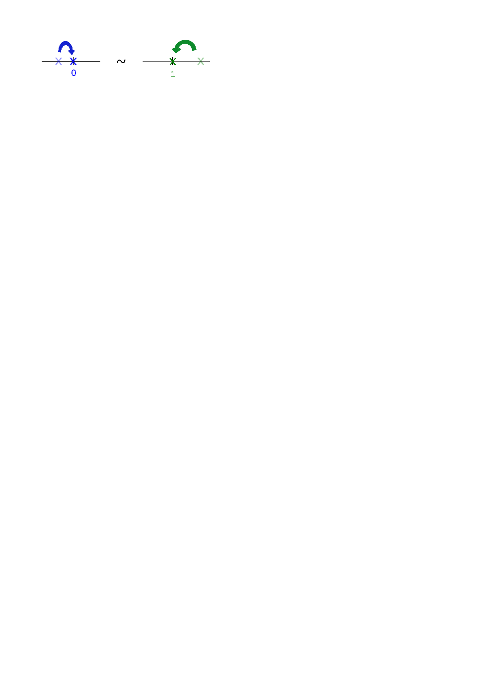
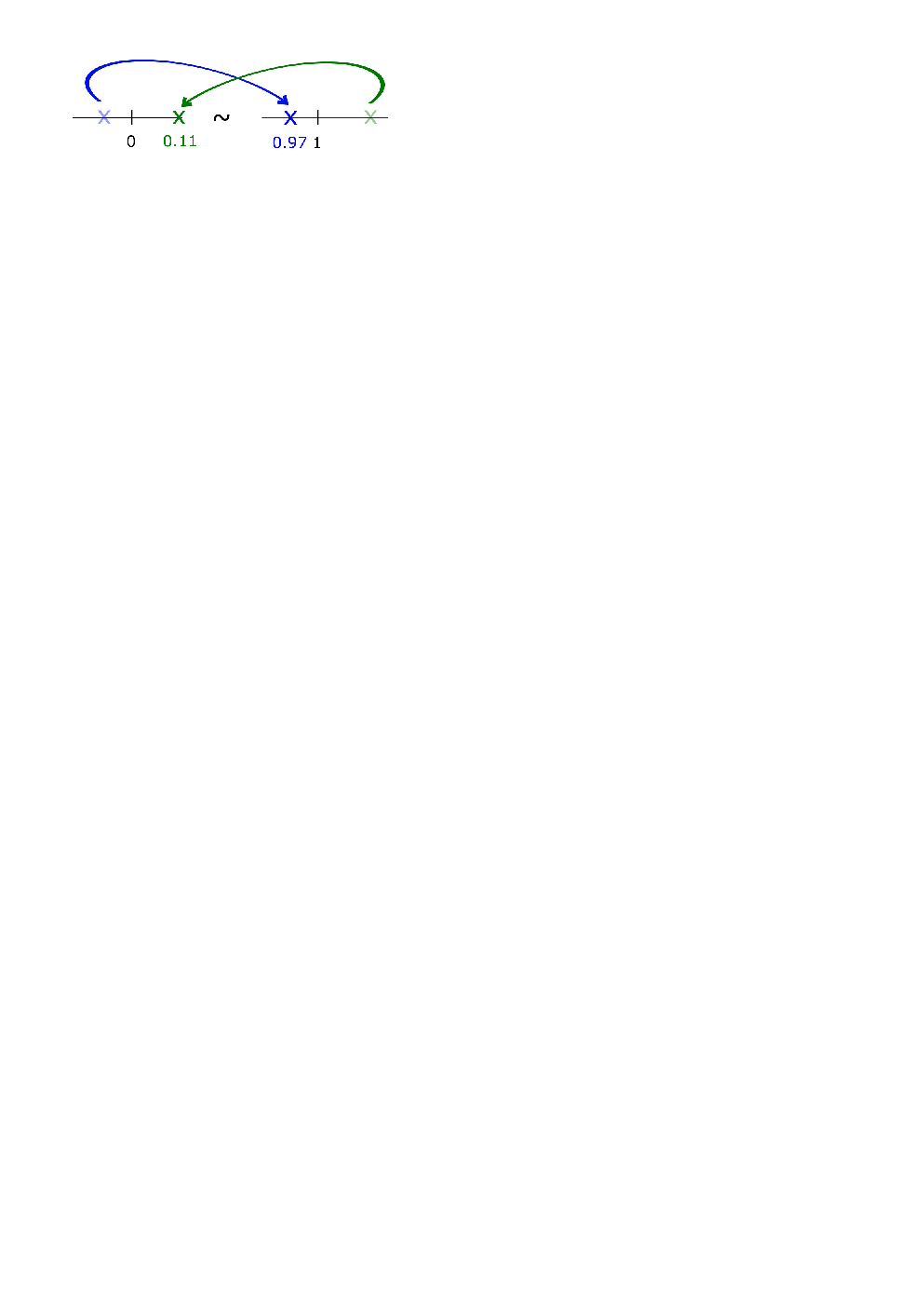
Furthermore, rather generally, all correction strategies can be further classified as either superficial or complete ones. Superficial correction strategies limit their impact to only reassigning coordinates of the out-of-domain points to be back within the domain without re-evaluating the resulting corrected point. Solutions corrected with such become in some sense “alien” to the original objective function – they are the artefacts of the design choice (a choice of correction strategy) rather then the objective function itself – and comparison of two algorithms employing drastically different correction strategies is akin comparing apples and the so-called “Chinese apples”.
Schematic explanation of examples of superficial correction strategies popular in the field of EA are shown in Figure 1.

Meanwhile, the complete correction strategies actively search for other feasible inside-the-domain points in the (relative) vicinity of the currently unfeasible point. This search is typically performed via some local search routine with prescribed complexity and budget of function evaluations. Thus, complete strategies ensure that corrected solutions fully represent the original objective function unlike the superficial strategies that only assign artificially fitness values to moved-previously-unfeasible points. However, complete correction strategies create “holes” in the domains that are filled with unfeasible points for which no quality information is provided to the optimisation method. This directly contradicts a long-standing idea of the EAs operating via combining partial information from all the population [33]. Use of complete correction strategies introduces further problems such as being extremely time-consuming or a possibility of transferring limitations of the chosen local search algorithm into a failure to find suitable solutions by the overall method. Moreover, there is a risk that domain boundaries end up being over-explored due to the locality of the search concentrated around the boundary region22 2 This highlights a subtle connection between the choice of correction strategy and structural bias. Results presented in this paper lead one to believe that, potentially, correction strategy plays an important role in the formation of structural bias of the method. In practice, mostly due to time limitations and unwillingness to introduce additional design choices, complete correction strategies are rarely used. Instead, under a widely spread assumption of the non-importance of the correction strategy, simple superficial corrections are typically preferred with no justification. We argue that such assumption is, in fact, erroneous.
We argue that in practice significantly more solutions end up requiring correction than what is usually assumed by an algorithm designer. The overall number of corrections required during the optimisation provides a (rough) estimate for a degree to which the actual function being optimised corresponds to the original function, thus, projecting the justification to use local information. In other words, an overly high number of corrections deprives the algorithm from using information about the local structure of the landscape under investigation in most critical boundary regions.
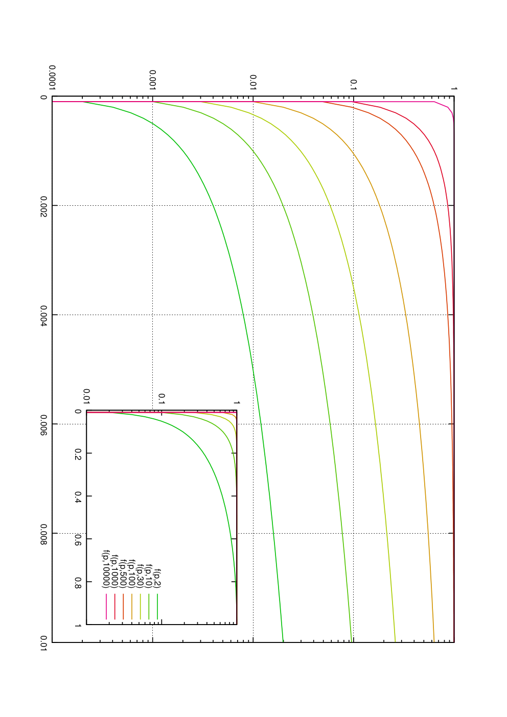
Clearly, a number of corrected solutions in the population grows with dimensionality of the problem since a solution with only one coordinate outside the domain already requires a correction. For a simplified experiment, suppose jumps outside the domain in different dimensions occur independently and with a constant rate 33 3 Obviously, this is a simplification of the real situation as this rate is not constant and there might be dependencies between dimensions.. Then probability of a solutions to require corrections in at least one dimension is then trivially expressed as , where is problem’s dimensionality. To help with visualisations, Figure 2 shows tabulations of this formula for various values of dimensionality (values of are shown in horizontal axis and – in vertical). It is easy to see that attains high values for relatively low values of and this effect is drastically increased as dimensionality increases. For a rather modest (by modern standards) value of dimensionality of , the probability that at some iteration a correction is required in at least one dimension exceeds for . As dimensionality increases further, virtually all solutions end up requiring corrections for majority of reasonable values of . This clearly demonstrates the importance of the correction strategy choice for high dimensional problems – thoughtlessly chosen correction strategy can transform the original optimisation problem into a trivial one which structurally has little to do with the original function.
Depending on the nature of the problem, some constraint handling technique choices might even become prohibitive: e.g. impossibility of keeping unfeasible solutions in the population in case of domain boundaries from physical limitations of some equipment used to compute objective function values. Thanks to design, some strategies may lead to identical behaviour for some algorithms (e.g. penalty and dismiss in DE, as explained in Section 4). For other strategies, performance of an algorithm can turn out to be drastically different with different constraint handling strategies as clearly demonstrated by results presented later in this paper. However, despite trivially achievable conclusions above, usually, the choice of constraint handling technique is not investigated thoroughly during the design of an optimisation algorithm. We aim to draw the attention of algorithm designers and practitioners to the importance of this choice. It turns out that as usual, it matters what happens on domain boundaries.
3 Differential Evolution
Differential Evolution is a powerful yet simple metaheuristic for global real-valued optimisation which only requires three parameters to function efficiently [55]: the scale factor , the crossover ratio and the population size . The DE framework consists of the iteration of only three steps, as shown in Algorithms 1. In the sense of “one-to-one-spawning” selection mechanism, it resembles the Swarm Intelligence methods such as PSO but, at the same time it is similar to the Evolutionary Algorithms such as the GA, as it requires a “mutation” operator, followed by a “croosover” strategy to produce a new solution.
Despite the lack of proper fitness-informed selection and a fixed order for the operator, a number of different algorithmic behaviours can be obtained from DE by changing and combining mutation and crossover operators. The most commonly used mutation operators are:
- 1.
rand/1:
(2) - 2.
rand/2:
(3) - 3.
best/1:
(4) - 4.
current-to-best/1:
(5)
Other configurations of DE exist and are described in the literature [48]. With reference to equations (2) to (3), indices are randomly sampled in order to pick the random individual from the populations.
In modern terminology, the initial version of DE proposed in 1995 is DE/rand/1/bin; it includes a “binomial” crossover where each variable has a prefixed probability to be exchanged. In subsequent implementations, a new crossover strategy has been proposed which exchanges bursts of consecutive components whose length depends on the value and the dimensionality of the problem. As the probability of exchanging one more coordinate in the burst follows the geometric progression, and thus it decays exponentially, this variant is commonly referred to as DE/rand/1/exp. Implementation details of bin and exp crossover strategies are given in Algorithm 2 and 3 respectively.
In modern terminology, any particular scheme can be obtained by combining the chosen mutation and crossover strategies which is reflected in the “DE/a/b/c” notation. The first member, “a”, refers to the vector being mutated (namely the one to which difference vectors are added), “b” is the number of difference vectors used and “c” indicates the crossover. For example, “a” could be “rand” (Formulas 2 and 3), “best” (Formulas 4) or even a combination of two vectors as in “current-to-best” (Formula 5).
Listed mutations provide a set of different moves across the search domain for handling different landscape scenarios. The current-to-best/1 strategy, for instance, can be of help in speeding up the convergence when dealing with less complex fitness functions (functions with plateau-like regions as opposed to highly multimodal or ill-conditioned functions) [9, 10]. However, it could be inadequate for highly multimodal functions, since it gives privilege to the direction towards the current best solution – a basic rand/1 would be preferred in this case.
Despite the low number of parameters in DE, their tuning plays a major role as performances can heavily depend on the parameter setting. A skilled algorithm designer may exploit these while designing hybrid structures, as the adequate combination of the scale factor and crossover rate can theoretically be used to control the kind of desired search, hence the “control parameters” name, so to reproduce either the more exploitative behaviours or the more local-search-like routine, simply by fine picking and . Unfortunately, this is not always achievable due to the lack of precise indications. The scale factor , which is used to control the exploitative lengths of mutations operators, has been initially thought to have a large range, i.e. , where the the value is usually not considered as it will nullify the effect of the difference vector of the mutation operator (see Formulas 2 to 5). On the contrary, the crossover rate has been expected to lie in the range , probabilistically, where extreme values are typically avoided to prevent the crossover operator to either replace only component(see Algorithm 2 and 3) or to return an exact copy of one of the parents. However, later on it has become more clear that only values of in were used in practical applications. Moreover, the subsequent study in [30] recommended and . In practice, users of DEs tend to settle on values close to for the scale factor and several DE algorithms have been proposed in which such parameters are self-adapted to the problem during the optimisation process [3], or picked up from a pool of promising values [13]. A key study in [59] has instead dug into the interrelation among parameters and and discovered an optimal tuning of the crossover rate in function of the scale factor.
Therefore, while research literature is rich of studies on setting and , significantly less information is available on setting the value of and some studies are also arguable. For example, [30] recommended to use a population made up of times the value of dimensionality of the problem. Such recommendation appears to be unfeasible in many real-world and large-scale scenarios [40], and, more importantly, it directly contradicts the observation that shrinking the population size can be beneficial to avoid stagnation [4].
Furthermore, large population size is known to promote diversity, thus reducing the risk of premature convergence [58]. However, a too large population size could potentially unnecessarily strengthen the deleterious effect of the structural bias. As demonstrated theoretically in [25] in case of GAs, the spread of the population across the domain is directly effected by the number of points in the population: unfortunately enough, as population size grows, so does the strength of structural bias. However, the situation is less clear for other optimisation frameworks and, in particular, for DE. According to the preliminary study in [7] such correlation is only partially confirmed. Surprisingly, it turned out that while the “current-to-best/1” mutation operator seems to carry a visible structural bias, a simpler “rand/1” is to some extent capable of mitigating the bias regardless of the chosen crossover strategy. Thus, [7] is extended here for a wider range of of aspects such as different parameter settings, corrections strategies and DE schemes.
4 Objectives, methods and experimental setup
The main objective of this publication is to analyses a wide range of popular DE configurations and identify a combination of mutation and crossover operators responsible for the rise of the structural bias in DE algorithms, as well as to observe to which extent the choice for the control parameters , , correction strategy and population size , can mitigate such bias. This knowledge can be exploited in the long term perspective to achieve a more informed algorithmic design process and to give practitioners guidance in tuning DE’s control parameters for real-world optimisation problems.
4.1 Choice of DE configurations
As explained in Section 2.2, identification of structural bias is based on the minimisation of function (1) 44 4 without loss of generality, conclusions here also hold true for the maximisation case. For historical reasons, dimensionality is kept at . To leave nothing to chance, the effect of different correction strategies is also taken into consideration in this study. Experiments in this article have been carried out with the following implementations of popular correction methods introduced in Section 2.3:
- 1.
penalise: is extended via a surjective penalty function mapping solutions outside the domain with a pre-fixed real valued constant :
(6) - 2.
- 3.
It must be pointed out that a popular “dismiss” correction strategy is indirectly omitted from this study as it would be equivalent to using a penalty function, due to the one-to-one spawning logic in DE. Indeed, in the most general case this is implemented as in Algorithm 6, in which the unfeasible solution is simply discarded and replaced with a parent chosen according to any convenient logic. However, the same replacement necessarily occurs in DE for penalised solutions as they are discarded based on a direct comparison on their fitness function value. Differently, it makes sense to differentiate between “penalise” and “dismiss” methods in EA paradigms such as e.g. some GAs for which selection takes place stochastic.
The mutation strategies presented in Section 3, Formulas 2 to 5, were combined with both bin and exp crossovers, i.e. Algorithms 2 and 3 respectively, thus, forming DE schemes. Each one was equipped with the aforementioned correction schemes (i.e. Formula 6, Algorithm 4 and 5) thus generating different DE configuration variants.
4.2 Choice of DE parameters
To decide on the most appropriate parameters settings for DE variants selected in the previous section, an extensive preliminary experimentation has been carried out. Keeping the number of runs and population sizes consistent with [25, 7], DE control parameters were investigated in the light of the percentage of points corrected throughout the whole optimisation process. The logic behind such investigation is to focus on the algorithmic behaviour and stick as much as possible to optimising the true thus minimising potential side effects introduced by the correction strategy. In this sense, percentage of corrections during the run is a metric of how aggressive, or badly-suited, the correction strategy is. On the other hand, the choice of control parameters of DE is balanced empirically by the fact that too few corrections potentially mean underexploitation of the domain boundaries as generating operators have relatively local nature. Thus, the most reliable - pair was determined by looking into pre-selected combinations of control parameters and , i.e. those generated with and . Such tabulation of the intervals of control parameters is empirically motivated by regions of particular interest.
This means that configurations of DE have been considered with population sizes each producing histograms (one per each couple) – resulting in full optimisation runs being performed each times to keep track of the percentage of occurred corrections. From distributions of these percentages of corrections, average and standard deviation surface plots have been produced to visually handle such amount of data and values of - of the control parameter couple have been chosen to force the algorithms under study to operate, as much as possible, within the problem’s boundaries. To avoid an unnecessarily long list of graphs here, all these results are made available online [8].
For demonstration purposes only, one example for the DE/rand/1/bin with penalty correction case and different population sizes is shown here in Figure 3. Detailed analysis of the percentage of corrections in different configurations of DE has proved to be very interesting and will be published shortly as a separate publication. To clarify, Figure 3 depicts distributions of the percentage of occurred corrections, while optimising , for each combination and (i.e. sub-diagrams per subfigure). Each sub-diagram carries two layers of information. The first layer, shown in red, represents the distribution of correction percentages in a series of runs. Percentages can be read on the y-axis (which points upwards and whose range is always ), while the number of runs is reported on x-axis (which points to the right). The second layer, shown in blue, indicates the employed values of and . Also for this layer, the y-axis points upwards and the x-xis to the right, but they report values for and respectively. For both layers, origin is in the lower left corner. This Figure attempts to draw a three-dimensional figure in projections in two dimensions: distributions shown in red in each small subfigure should be placed on the page in a perpendicular fashion towards the reader, in points marked in blue circles. Choice of number of bins in histograms is based on the investigation explained in the next section.


To summarise, having chosen appropriate values of DE control parameters, for the purpose of studying structural bias in DE configurations, all aforementioned DE configuration variants were each run times on for the dimensional case with a standard computational budget of fitness functional calls with , and population size of . Thus, in total, optimisation processes were repeated for runs to generate the results shown in Section 5.
4.3 Choice of granularity
To generate meaningful distribution figures such as Figure 3, it has become clear that bin size had to be tuned. Choosing a number of bins for a histogram is a balancing act which depends on the number of points in a histogram and features of the underlying true distribution of data (symmetry, skewness, etc.). Choosing a too small number of bins oversmooths the resulting histogram and potentially looses the distribution features. Meanwhile, a too high number of bins results in a too noisy picture which is difficult to interpret and generalise. Clearly, the number of bins should not exceed the number of data points. As no educated a priori assumptions could be made regarding properties of the distribution of the percentage of corrections, an initial study has been made to decide on the appropriate number of bins in distribution plots. DE/best/1/bin configuration with saturation correction has been chosen as representative and distributions of the percentage of corrections have been visualised for three population sizes for three different numbers of bins (, , ), see Fig. 4.


Clearly, histograms with bins (last row in Fig. 4) are too noisy. Histograms with bins (middle row in Fig. 4) barely show any qualitative differences with bins, thus they are too noisy as well. Histograms with bins (top row in Fig. 4) are too crude. Thus, it has been decided to use bins for all histograms of the percentage of corrections as is done in Figure 3.
4.4 Further results on distributions of the number of corrections
To help with visualising multidimensional data, Figures 5 depicts the average percentage of corrections for DE/rand/1/bin configuration, over runs, for three population sizes, occurring for each one of the combination. More specifically, in each subfigure, axes pointing upwards shows values of , meanwhile axis pointing to the right shows values of . Colour encodes the value of the a posteriori computed average percentage of corrections for experiments with given and values – experimentally obtained values of averages are marked with small dots, meanwhile averages for the rest of couples are interpolated and smoothed. Black curves are interpolated contour curves for the average percentage of corrections. Colour axis is the same for all subfigures – it runs from values in blue to values in green. Chosen paid is marked with a small circle.


Similarly, Figure 6 shows standard deviation of the percentage of corrections if DE/rand/1/bin configuration, over runs, for three population sizes, occurring for each one of the combination. More specifically, in each subfigure, axes pointing upwards shows values of , mean while axis pointing to the right shows values of . Colour encodes the value of the a posteriori computed standard deviation of percentage of corrections for experiments with given and values – experimentally obtained values of standard deviation are marked with small dots, meanwhile standard deviations for the rest of couples are interpolated and smoothed. Black curves are interpolated contour curves for the standard deviation of the percentage of corrections. Colour axis is the same for all subfigures – it runs from values in yellow to values in violet. Chosen paid is marked with a small circle.


As mentioned previously, detailed analysis of the distributions, averages and standard deviations in the percentage of corrections for different configurations of DE will be published shortly as a separate publication. However, it is worth mentioning now that, unexpectedly, at least from the point of view of the analysis of the percentages of corrections, control parameters of DE seem to have different and, moreover, usually opposite effect in different configurations of DE. In other words, what our results show is that, from the point of view of dynamics, DE, in effect, is transformed into a different algorithm with the change of it’s configuration – dynamics inside DE drastically depends on the inner structure of the operators.
Apart from other conclusions, this also means that it is hardly ever sensible to talk about ”tuning control parameters for DE” in general. For example, high values of do not necessarily always mean large steps of the algorithm as popular research suggests [26] – if it was so, the number of corrections would consistently be high for all DE configurations, regardless the chosen value of as higher number of larger steps correlates with the higher numbers of corrections. Our results suggest that it is not the case – higher number of corrections is indeed attained for higher values of but for some configurations this consistently happens for higher values of and for some – for low values of . Clearly, more research is required in this direction.
5 Results on structural bias
Graphical results have been generated as explained in Section 2.2 and grouped according to the specific DE scheme in the file [8] for visual inspection. To facilitate their analysis, the possible configurations of correction strategies and population size are positioned in the same page, thus giving a general view of each one of the DE configurations considered in this study.
A glance at these results immediately brings out clear differences between DE/current-to-best/1/bin and the other schemes under examination, as it is the only configuration to display a clear structural bias. All biased patterns have been grouped Figure 7 in contrast to Figure 8 where some of the remaining unbiased patterns are showed.


Thus, after the first observation, one must conclude that Differential Evolution is a robust and less biased optimisation paradigm with respect to others, such as e.g. GA and PSO examined in [25]. Furthermore, it appears that classic DE schemes present weaker biases than some modern self-adaptive approaches as the JADE algorithm [44]. Most importantly, it is interesting to note that simpler mutation schemes, as DE/rand/1, DE/rand/2 and DE/best/1, do not seem to carry significant structural biases neither when the binomial crossover is employed, nor when it is replaced with the exponential one (see top row of Figure 8). Moreover, they are not sensitive to the choice for the correction strategy and despite what observed in [25] – where the strength of the structural bias increases with increasing population sizes in GA and PSO based optimisation – the number of individuals seems not to have a direct impact on the biases of these algorithmic structures (see bottom layer of Figure 8).


Conversely, it is evident that DE/current-to-best/1/bin tends to privilege specific regions as the best individuals accumulate towards the centre of the search space at the end of the optimisation process. Once again, in contrast to what was previously observed in [25], the displayed bias seems to only marginally depend on the population size, as can be seen from Figure 7. It must be pointed out that even though this knowledge was already available from the preliminary study in [7], in which saturation and toroidal corrections were employed, a peculiar behaviour arose in this examination while trying the penalty approach of Formula 6, so eliminating its structural bias (see Figure 9). It must be remarked that a similar result cannot be easily obtained with different optimisation paradigms. This is graphically shown in Figures 9(d) which displays a visible, albeit not strong, structural bias for a GA equipped with penalty correction.


Interestingly enough, results obtained with different population sizes and different correction strategies further confirmed the “mitigating” effect of the crossover operator for the structural bias of DE/current-to-best/1 [7]. Indeed, see the bottom row of Figure 8, DE/current-to-best/1/exp unexpectedly appears not to be biased at all by visual inspection. A motivation for this discrepancy can be attributed to the fact that, for a given value, the average number of exchanged design variables is higher if the binomial crossover is used, whereas it is lower in presence of the exponential crossover. The latter logic is indeed based on a different working principle according to which the probability of exchanged components decays exponentially and depends on the dimension of the problem – a fair comparison between two DE algorithms employing bin and exp crossovers should consider the ad-hoc crossover rates and respectively [10]. This means that, for the considered dimension value , only a few components are in fact exchanged. One can therefore speculate that such a low value is simply not enough to manifest a visible structural bias. However, this should not be the case as it would implies that only the crossover operator, and in particular the binomial one, introduces biases into the DE framework while all considered mutation strategies are unbiased. At the current state of this investigation, this does not seem to be reasonable considering that both the bin and exp options have been used with other mutation schemes in this study but clear biases, visible by the naked eye, were not individuated.
The latter considerations suggest that the structural bias of an optimisation algorithm is not simply the result of the sum of biases of its operators and can also arise under particular mutation-crossover combinations, or in general, under specific combination of both biased and unbiased operators. In this light, the structural bias can also be seen as a non-linear phenomenon where the biases of two biased operators does not necessarily add up if they are combined within an algorithm, but rather generate spurious contributions biasing the search further and differently.
6 Conclusions
This paper systematically analyses a wide range of popular DE configurations in the light of structural bias that manifest itself during optimisation process as the algorithm “preferring” some regions of the search space to the others. Such behaviours has been clearly demonstrated in other EA algorithms and shown to stem from iterative application of algorithmic operators, each potentially plagued with their own shortcomings. These shortcomings are thus superimposed by the algorithm’s structure and could thus limit the overall performance of the algorithm due to an uneven exploration of the search space.
Compared to previous studies, a new aspect usually overlooked during algorithmic design stage is considered as potential contributor to the formation of structural bias – choice of constraint handling technique – which has eventually turned out to be crucial in mitigating the effects of structural bias on an otherwise highly biased DE configuration. This is evident in DE/current-to-best/1/bin whose bias can be eliminated by simply employing the penalty constraint handling strategy. In this light, practitioners are recommended to use DE/current-to-best/1/bin in combinations with such constraint handling method, and also algorithm designers to pay more attention to the often underestimated details which could, surprisingly, make the big difference.
Triggering mechanisms of structural bias in DE has also turned out to be different from that of GA and PSO – population size has no clear effect on the strength of structural bias. Main results suggest that the structural bias of an optimisation algorithm is really a superposition and not a sum of effects of individual operators as in general it can arise from a specific combination of both biased and unbiased operators generating spurious contributions and biasing the search further and in a different manner.
In the future, promising areas of investigations are then two-folded: first, to examine the contribute of algorithmic operators (in support of our observation that the system as a whole can be biased regardless of the single component), their structural bias has to be searched and quantified; second, alternative ways to visualise/quantify bias, e.g. clustering, can be designed to flag critical cases and confirm the absence/presence of structural bias. These would clarify unsolved matters and helps understand the triggering mechanism for the bias, not only in DE.
Results presented in this paper have also suggested an interesting direction for future research – interpretation of dynamics inside the DE population based on proxy estimates and subsequent interpretation of the control parameters pair. To the best of our knowledge, to date, such interpretation valid for all DE configurations is still missing.
References
- Andre et al. [2001] Andre, J., Siarry, P., Dognon, T., 2001. An improvement of the standard genetic algorithm fighting premature convergence in continuous optimization. Advances in engineering software 32 (1), 49–60.
- Angeline [1998] Angeline, P. J., May 1998. Using selection to improve particle swarm optimization. In: 1998 IEEE International Conference on Evolutionary Computation Proceedings. IEEE World Congress on Computational Intelligence (Cat. No.98TH8360). pp. 84–89.
- Brest et al. [2006] Brest, J., Greiner, S., Bošković, B., Mernik, M., Žumer, V., Dec 2006. Self-adapting control parameters in differential evolution: A comparative study on numerical benchmark problems. IEEE Transactions on Evolutionary Computation 10 (6), 646–657.
- Brest and Maučec [2008] Brest, J., Maučec, M. S., 2008. Population size reduction for the differential evolution algorithm. Applied Intelligence 29 (3), 228–247.
- Burke et al. [2019] Burke, E. K., Hyde, M. R., Kendall, G., Ochoa, G., Özcan, E., Woodward, J. R., 2019. A classification of hyper-heuristic approaches: Revisited. In: Handbook of Metaheuristics. Springer, pp. 453–477.
- Caraffini [2016]
Caraffini, F., 5 2016. Algorithmic issues in computational intelligence
optimization: from design to implementation, from implementation to design.
No. 243 in Jyväskylä studies in computing. University of
Jyväskylä.
URL http://urn.fi/URN:ISBN:978-951-39-6742-0 - Caraffini and Kononova [2018] Caraffini, F., Kononova, A., 18-21 September 2018. Structural bias in differential evolution: a preliminary study. In: LeGO 2018 - 14th International Workshop on Global Optimization, Leiden, The Netherlands. AIP.
- Caraffini et al. [2019] Caraffini, F., Kononova, A. V., Corne, D., 2019. Infeasibility and structural bias in differential evolution. www.cse.dmu.ac.uk/˜fcaraf00/BIAS/BIAS_DE_EXTENDED_RESULTS.pdf.
- Caraffini and Neri [2018a] Caraffini, F., Neri, F., 2018a. Rotation invariance and rotated problems: An experimental study on differential evolution. In: Sim, K., Kaufmann, P. (Eds.), Applications of Evolutionary Computation. Springer International Publishing, Cham, pp. 597–614.
- Caraffini and Neri [2018b] Caraffini, F., Neri, F., 2018b. A study on rotation invariance in differential evolution. Swarm and Evolutionary Computation.
- Caraffini et al. [2014] Caraffini, F., Neri, F., Picinali, L., 2014. An analysis on separability for memetic computing automatic design. Information Sciences 265 (0), 1 – 22.
- Chen, Ti-Hung et al. [2017] Chen, Ti-Hung, Yeh, Ming-Feng, Lee, Wen-Yo, 2017. Particle swarm optimization based networked control system design with uncertainty. MATEC Web Conf. 119, 01051.
- Cheng et al. [2015] Cheng, J., Zhang, G., Caraffini, F., Neri, F., 2015. Multicriteria adaptive differential evolution for global numerical optimization. Integrated Computer-Aided Engineering 22 (2), 103–107.
- Davarynejad et al. [2014] Davarynejad, M., van den Berg, J., Rezaei, J., 2014. Evaluating center-seeking and initialization bias: The case of particle swarm and gravitational search algorithms. Information Sciences 278, 802 – 821.
- de Oca et al. [2009] de Oca, M. A. M., Stützle, T., Birattari, M., Dorigo, M., 2009. Frankenstein’s PSO: A composite particle swarm optimization algorithm. IEEE Transactionon on Evolutionary Computation 13 (5), 1120–1132.
- Eiben and Smit [2011] Eiben, A., Smit, S., 2011. Parameter tuning for configuring and analyzing evolutionary algorithms. Swarm and Evolutionary Computation 1 (1), 19 – 31.
- Eiben and Smith [2003] Eiben, A. E., Smith, J. E., 2003. Introduction to Evolutionary Computation. Springer-Verlag, Berlin, Germany.
- Grippo and Rinaldi [2015] Grippo, L., Rinaldi, F., 2015. A class of derivative-free nonmonotone optimization algorithms employing coordinate rotations and gradient approximations. Comp. Opt. and Appl. 60, 1–33.
- Iacca et al. [2013] Iacca, G., Caraffini, F., Neri, F., 2013. Memory-saving memetic computing for path-following mobile robots. Applied Soft Computing 13 (4), 2003 – 2016.
- Iacca et al. [2012] Iacca, G., Caraffini, F., Neri, F., Mininno, E., April 2012. Robot base disturbance optimization with compact differential evolution light. In: et al., D. C. C. (Ed.), Applications of Evolutionary Computation. EvoApplications 2012. Lecture Notes in Computer Science, vol 7248. Springer, Berlin, Heidelberg, pp. 285–294.
- Inselberg [1985] Inselberg, A., Aug 1985. The plane with parallel coordinates. The Visual Computer 1 (2), 69–91.
- Janson and Middendorf [2007] Janson, S., Middendorf, M., April 2007. On trajectories of particles in pso. In: 2007 IEEE Swarm Intelligence Symposium. pp. 150–155.
- Kennedy [2007] Kennedy, J., April 2007. Some issues and practices for particle swarms. In: IEEE Swarm Intelligence Symposium SIS 2007. pp. 162–169.
- Kim et al. [2007] Kim, H., Chong, J., Park, K., Lowther, D. A., April 2007. Differential evolution strategy for constrained global optimization and application to practical engineering problems. IEEE Transactions on Magnetics 43 (4), 1565–1568.
- Kononova et al. [2015] Kononova, A. V., Corne, D. W., Wilde, P. D., Shneer, V., Caraffini, F., 2015. Structural bias in population-based algorithms. Information Sciences 298, 468–490.
- Lampinen and Zelinka [2000] Lampinen, J., Zelinka, I., 2000. On stagnation of the differential evolution algorithm. In: Oŝmera, P. (Ed.), Proceedings of International Mendel Conference on Soft Computing. pp. 76–83.
- Larik and Haider [2016] Larik, A. S., Haider, S., Nov 2016. On using evolutionary computation approach for strategy optimization in robot soccer. In: 2016 2nd International Conference on Robotics and Artificial Intelligence (ICRAI). pp. 11–16.
- L’Ecuyer [1999] L’Ecuyer, P., 1999. Tables of linear congruential generators of different sizes and good lattice structure. Mathematcs of computation 68 (225), 249–260.
- Leung et al. [1997] Leung, Y., Gao, Y., Xu, Z.-B., 1997. Degree of population diversity- a perspective on premature convergence in genetic algorithms and its markov chain analysis. IEEE Transactions on Neural Networks 8 (5), 1165–1176.
- Liu and Lampinen [2005] Liu, J., Lampinen, J., Jun 2005. A fuzzy adaptive differential evolution algorithm. Soft Computing 9 (6), 448–462.
- Malan and Engelbrecht [2013] Malan, K. M., Engelbrecht, A. P., 2013. A survey of techniques for characterising fitness landscapes and some possible ways forward. Information Sciences 241, 148–163.
- Mason et al. [2018] Mason, K., Duggan, J., Howley, E., 2018. A meta optimisation analysis of particle swarm optimisation velocity update equations for watershed management learning. Applied Soft Computing 62, 148 – 161.
- Michalewicz [1995] Michalewicz, Z., 1995. A survey of constraint handling techniques in evolutionary computation methods. Evolutionary programming 4, 135–155.
- Miettinen [1999] Miettinen, K. (Ed.), 1999. Evolutionary Algorithms in Engineering and Computer Science: Recent Advances in Genetic Algorithms, Evolution Strategies, Evolutionary Programming, GE. John Wiley & Sons, Inc., New York, NY, USA.
- Molina et al. [2010] Molina, D., Lozano, M., García-Martínez, C., Herrera, F., mar 2010. Memetic algorithms for continuous optimisation based on local search chains. Evolutionary Computing 18 (1), 27–63.
- Monson and Seppi [2005] Monson, C. K., Seppi, K. D., 2005. Exposing origin-seeking bias in PSO. In: GECCO’05. pp. 241–248.
- Nannen and Eiben [2006] Nannen, V., Eiben, A., 2006. A method for parameter calibration and relevance estimation in evolutionary algorithms. In: Proceedings of the 8th Annual Conference on Genetic and Evolutionary Computation. GECCO ’06. ACM, New York, NY, USA, pp. 183–190.
- Ong et al. [2010] Ong, Y., Lim, M. H., Chen, X., May 2010. Memetic computation—past, present amp; future [research frontier]. IEEE Computational Intelligence Magazine 5 (2), 24–31.
- Orvosh and Davis [1993] Orvosh, D., Davis, L., 1993. Shall we repair? genetic algorithmscombinatorial optimizationand feasibility constraints. In: Proceedings of the 5th International Conference on Genetic Algorithms. Morgan Kaufmann Publishers Inc., San Francisco, CA, USA, pp. 650–.
- Parsopoulos [2009] Parsopoulos, K. E., 2009. Cooperative micro-differential evolution for high-dimensional problems. In: Proceedings of the conference on Genetic and evolutionary computation. pp. 531–538.
- Peng et al. [2010] Peng, F., Tang, K., Chen, G., Yao, X., 2010. Population-based algorithm portfolios for numerical optimization. IEEE Transactionon on Evolutionary Computation 14 (5), 782–800.
- Piotrowski and Napiorkowski [2016] Piotrowski, A. P., Napiorkowski, J. J., Dec 2016. Searching for structural bias in particle swarm optimization and differential evolution algorithms. Swarm Intelligence 10 (4), 307–353.
- Piotrowski and Napiorkowski [2018a] Piotrowski, A. P., Napiorkowski, J. J., 2018a. Some metaheuristics should be simplified. Information Sciences 427, 32 – 62.
- Piotrowski and Napiorkowski [2018b] Piotrowski, A. P., Napiorkowski, J. J., 2018b. Step-by-step improvement of jade and shade-based algorithms: Success or failure? Swarm and Evolutionary Computation.
- Poikolainen et al. [2015] Poikolainen, I., Neri, F., Caraffini, F., 2015. Cluster-based population initialization for differential evolution frameworks. Information Sciences 297, 216–235.
- Poli and Graff [2009] Poli, R., Graff, M., 2009. There is a free lunch for hyper-heuristics, genetic programming and computer scientists. In: Vanneschi, L., Gustafson, S., Moraglio, A., De Falco, I., Ebner, M. (Eds.), Genetic Programming. Vol. 5481 of Lecture Notes in Computer Science. Springer Berlin Heidelberg, pp. 195–207.
- Powell [1964] Powell, M. J. D., Jan. 1964. An efficient method for finding the minimum of a function of several variables without calculating derivatives. The Computer Journal 7 (2), 155–162.
- Price et al. [2005] Price, K. V., Storn, R., Lampinen, J., 2005. Differential Evolution: A Practical Approach to Global Optimization. Springer.
- Prügel-Bennett [2010] Prügel-Bennett, A., 2010. Benefits of a population: Five mechanisms that advantage population-based algorithms. IEEE Transactions on Evolutionary Computation 14 (4), 500–517.
- Quagliarella et al. [1997] Quagliarella, D., Périaux, J., Poloni, C., Winter, G., 1997. Genetic algorithms and evolution strategies in engineering and computer science. Jhon Wiley & Sons.
- Rahmat-Sami and Jin [2007] Rahmat-Sami, Y., Jin, N., Sept 2007. Particle swarm optimization (pso) in engineering electromagnetics: A nature-inspired evolutionary algorithm. In: 2007 International Conference on Electromagnetics in Advanced Applications. pp. 177–182.
- Rudolph [2001] Rudolph, G., 2001. Self-adaptive mutations may lead to premature convergence. IEEE Transactions on Evolutionary Computation 5 (4), 410–414.
- Spall [1992] Spall, J. C., 1992. Multivariate stochastic approximation using a simultaneous perturbation gradient approximation. IEEE Transactions on Automatic Control 372, 332–341.
- Spears et al. [2010] Spears, W., Green, D., Diana F., S., 11 2010. Biases in particle swarm optimization. International Journal of Swarm Intelligence Research (IJSIR) 1, 34–57.
- Storn and Price [1995] Storn, R., Price, K., 1995. Differential evolution - a simple and efficient adaptive scheme for global optimization over continuous spaces. Tech. Rep. TR-95-012, ICSI.
- Stutzle and Dorigo [2002] Stutzle, T., Dorigo, M., Aug 2002. A short convergence proof for a class of ant colony optimization algorithms. IEEE Transactions on Evolutionary Computation 6 (4), 358–365.
- Wolpert and Macready [1997] Wolpert, D., Macready, W., 1997. No free lunch theorems for optimization. IEEE Transactions on Evolutionary Computation 1, 67–82.
- Yaman et al. [2018] Yaman, A., Iacca, G., Caraffini, F., 18-21 September 2018. A comparison of three differential evolution strategies in terms of early convergence with different population sizes. In: LeGO 2018 - 14th International Workshop on Global Optimization, Leiden, The Netherlands. AIP.
- Zaharie [2002] Zaharie, D., 2002. Critical values for control parameters of differential evolution algorithm. In: Matuŝek, R., Oŝmera, P. (Eds.), Proceedings of 8th International Mendel Conference on Soft Computing. pp. 62–67.
- Zhou et al. [2007] Zhou, Z., Ong, Y. S., , Lim, M. H., 2007. Memetic algorithm using multi-surrogates for computationally expensive optimization problems. Soft Computing 11, 957–971.