跳到论文正文
W Papers独立论文阅读器 arXiv:1901.06124 论文正文 计算阅读时间 · 0%
引用这篇论文根据当前论文元数据生成,正式投稿前建议核对。


License: arXiv.org perpetual non-exclusive license
arXiv:1901.06124v1 [quant-ph] 18 Jan 2019

Continuum Limits of Quantum Lattice Systems

Tobias J. Osborne Affiliation: Institut für Theoretische Physik, Leibniz Universität Hannover, Appelstr. 2, 30167 Hannover, Germany
Abstract

We describe a general procedure to give effective continuous descriptions of quantum lattice systems in terms of quantum fields. There are two key novelties of our method: firstly, it is framed in the hamiltonian setting and applies equally to distinguishable quantum spins, bosons, and fermions and, secondly, it works for arbitrary variational tensor network states and can easily produce computable non-gaussian quantum field states. Our construction extends the mean-field fluctuation formalism of Hepp and Lieb (developed later by Verbeure and coworkers) to identify emergent continuous large-scale degrees of freedom — the continuous degrees of freedom are not identified beforehand. We apply the construction to to tensor network states, including, matrix product states and projected entangled-pair states, where we recover their recently introduced continuous counterparts, and also for tree tensor networks and the multi-scale entanglement renormalisation ansatz. Finally, extending the continuum limit to include dynamics we obtain a strict light cone for the propagation of information.

The modern understanding of quantum field theory (QFT), emphasised by Wilson Wilson 1975, is as an effective theory describing large lengthscale physics. Thus it has become a powerful tool for the description of the behaviour of complex quantum systems, including, critical phenomena Sachdev 2011 and topological order Wen 2007. Quantum-field reasoning is especially powerful when the system is effectively modelled by a weakly interacting QFT, enabling the full power of perturbative methods to be unleashed. Unfortunately, however, the QFT approach is not a universal panacea: when one obtains a strongly coupled effective QFT description, e.g., a nonabelian gauge theory, then perturbative methods are not so easily applied and one must resort to numerical methods, largely obviating the simplifications afforded by the effective continuous description 11 1 Note that there are very powerful general methods based on the supersymmetric method Efetov 1997, and yet others on the AdS/CFT correspondence Sachdev 2010, that can be exploited in the nonperturbative regime.. In such cases a tensor network Orús 2014; Bridgeman and Chubb 2017 may afford a more parsimonious representation for the physics of the system.

Tensor network states (TNS) have enjoyed, thanks to insights from quantum information theory in the study of entanglement, a recent renaissance allowing the analytic and numerical investigation of many intriguing strongly correlated phenomena, including, dynamics Vidal 2003; Haegeman et al. 2011; Osborne 2006, fermions Corboz and Vidal 2009; Corboz et al. 2010a; Corboz et al. 2010b; Kraus et al. 2010 without sign problems, the determination of spectral information Haegeman et al. 2012, topological order Aguado and Vidal 2008; Buerschaper et al. 2009; König et al. 2009, and dissipative quantum phenomena Verstraete et al. 2004; Zwolak and Vidal 2003; Kraus and Osborne 2012. There are, however, many remaining challenges. One outstanding problem is that it is difficult to identify the correct effective continuous degrees of freedom describing the experimentally relevant long-range behaviour of a TNS Verstraete and Cirac 2010; Haegeman et al. 2013; Jennings et al. 2015. Thus it is desirable to develop a more systematic and operationally well-motivated procedure to obtain an effective continuous description. Such a method, if developed, would also potentially contribute to the study of nonperturbative QFT because the TNS ansatz could then be systematically lifted to the continuous setting potentially giving new computable nongaussian vacua.

One standard way to obtain an effective QFT description of a system is based on the use of the path-integral representation (see, e.g., Wilson 1975; Auerbach 1994): one first represents the partition function using the path integral. Effective large-lengthscale continuous degrees of freedom are then identified and the path integral approximated by a continuum field path integral. This procedure has been applied with considerable success to a tremendous variety of lattice systems (see, e.g., Sachdev 2011; Fradkin 2013). However, this approach does not apply so readily to systems efficiently described in terms of tensor network states. Although there are now path-integral representations for several TNS classes Brockt et al. 2012; Jennings et al. 2015, it is not clear how to use this representation to identify the relevant degrees of freedom for such a network. It is almost certainly a red herring to exploit a stationary phase argument for the path integral representation here as this could easily identify auxiliary degrees of freedom which lead to trivial changes in the physical state. Indeed, the question of identifying the operationally relevant degrees of freedom for the description of the large-scale features of a complex quantum system has only recently been initiated Bény and Osborne 2013; Bény 2017.

In this Letter we describe a construction which produces an effective continuous description of a quantum lattice system whether it be in a TNS or a gaussian state. The first step is to identify a classical mean-field like continuous description, which we do by exploiting a generalised mean-field approach along the lines of Verbeure 2011 and Raggio and Werner 1989; Raggio and Werner 1991. The operationally significant quantum fluctuations around this classical state are then identified and represented in terms of a family quantum fields in a systematic way. We achieve this by generalising the quantum fluctuation algebra construction originated by Hepp and Lieb Hepp and Lieb 1973 (later generalised by Verbeure and coworkers Goderis et al. 1989a; Goderis and Vets 1989; Goderis et al. 1990a; Goderis et al. 1989b; Goderis et al. 1990b; Goderis et al. 1988; Goderis et al. 1989c; Michoel et al. 1998; Requardt 2002; Verbeure 2011) to produce a quantum field fluctuation algebra. The result of this construction is a list of quantum-field data for the system: (i) a quantum field “ground state” |Ω⟩|\Omega\rangle; and (ii) a list of quantum fields for the fluctuations with a precise map to the corresponding lattice quantities. This construction may be applied to matrix product states, projected entangled-pair states, and tree-type tensor networks such as the multiscale entanglement renormalization ansatz. (When applied to quasi-free lattice systems such as the lattice Klein-Gordon equation, one recovers the usual QFT continuum limit.) Extending the continuum limit to apply to dynamics we obtain strict causality: information may not propagate outside of a light-cone.

Preliminaries

.—Our construction applies to systems arranged on a lattice a​ℤDa\mathbb{Z}^{D} embedded in ℝD\mathbb{R}^{D}, where a>0a>0 is the lattice spacing. For simplicity we mostly restrict to one-dimensional quantum spin systems with a single distinguishable quantum spin ℂd\mathbb{C}^{d} attached to each site. (These assumptions entail no essential restrictions: all our subsequent constructions apply immediately to higher-dimensional systems and even to irregular lattices embedded in ℝD\mathbb{R}^{D}.) Thus the Hilbert space for our system is morally associated with the infinite tensor product ⨂j∈ℤℂd\bigotimes_{j\in\mathbb{Z}}\mathbb{C}^{d}. Considerable care should be exercised when working with such tensor products; the safest course of action, and the one adopted here, is to work with the space 𝒜⁡(ℤ)\mathcal{A}(\mathbb{Z}) of observables of the spin system instead 22 2 Let d∈ℕd\in\mathbb{N} and x∈ℤDx\in\mathbb{Z}^{D} and write 𝒜x≅Md​(ℂ)\mathcal{A}_{x}\cong M_{d}(\mathbb{C}), where Md​(ℂ)M_{d}(\mathbb{C}) is the algebra of d×dd\times d complex matrices. Then for any finite subset Λ⊂ℤD\Lambda\subset\mathbb{Z}^{D} let 𝒜⁡(Λ)\mathcal{A}(\Lambda) be the tensor product of 𝒜x\mathcal{A}_{x} over all x∈Λx\in\Lambda. For Λ1⊂Λ2\Lambda_{1}\subset\Lambda_{2} identify 𝒜⁡(Λ1)\mathcal{A}(\Lambda_{1}) with the subalgebra 𝒜⁡(Λ1)⊗𝕀Λ2∖Λ1⊂𝒜⁡(Λ2)\mathcal{A}(\Lambda_{1})\otimes\mathbb{I}_{\Lambda_{2}\setminus\Lambda_{1}}\subset\mathcal{A}(\Lambda_{2}). For infinite Λ⊂ℤD\Lambda\subset\mathbb{Z}^{D} denote by 𝒜⁡(Λ)\mathcal{A}(\Lambda) the C∗C^{*}-closure of the increasing family of finite-dimensional algebras 𝒜⁡(Λf)\mathcal{A}(\Lambda_{f}) with Λf⊂Λ\Lambda_{f}\subset\Lambda. The quasi-local algebra is then 𝒜⁡(ℤD)\mathcal{A}(\mathbb{Z}^{D})..

Let j∈ℤj\in\mathbb{Z} and A∈𝒜≡Md​(ℂ)A\in\mathcal{A}\equiv M_{d}(\mathbb{C}). Then we usually write AjA_{j} for the observable AA localised at spin jj: Aj≡𝕀⋯j−2,j−1⊗Aj⊗𝕀j+1,j+2,⋯A_{j}\equiv\mathbb{I}_{\cdots j-2,j-1}\otimes A_{j}\otimes\mathbb{I}_{j+1,j+2,\cdots}. We often require a basis for 𝒜\mathcal{A}: to this end let λα\lambda^{\alpha} be an orthonormal hermitian operator basis for the single-site observables 𝒜\mathcal{A} (according to the Hilbert-Schmidt inner product).
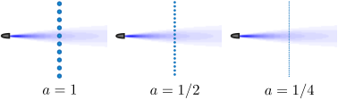
Refer to caption
Figure 1: An illustration of the continuum limit: measuring the observable ϕ(a)​(fx)\phi^{(a)}(f_{x}). Here the quantum lattice is illustrated for several different values of the lattice spacing aa. As aa gets smaller any fixed measurement of the quantum spin centred on xx will necessarily address more and more spins. The continuum limit is given by a limiting value ϕ⁡(fx)\phi(f_{x})
The classical continuum limit

.—The key to understanding how to take a continuum limit is to work out an operationally meaningful way to compare states ρa\rho_{a} and ρa′\rho_{a^{\prime}} associated with different lattice spacings a≠a′a\not=a^{\prime}. Naively this is impossible unless a=a′a=a^{\prime} because the quantum spins typically live at different locations. The crucial idea here is to compare states not directly by the fidelity but by instead agreeing on a family of observables {Oa}a∈ℝ+\{O_{a}\}_{a\in\mathbb{R}^{+}}, indexed by aa, which are understood to refer to the same experiment, only discretised on a lattice with spacing aa. If ρa​(Oa)≈ρa′​(Oa′)\rho_{a}(O_{a})\approx\rho_{a^{\prime}}(O_{a^{\prime}}) for all observables OaO_{a} then we declare the two states to be close. A physical justification for this notion is as follows. Imagine we have a quantum spin chain and we perform a neutron-type scattering experiment (see Fig. 1 for an illustration) to measure, for example, the zz-component of a spin at physical position xx. The impinging beam of neutrons, even if well collimated, will inevitably spread as it travels toward the spin chain. Thus the observable measured by this scattering experiment is, instead of σ⌊x/a⌋z\sigma^{z}_{\lfloor x/a\rfloor}, rather something like ϕ(a)​(fx)≡a​∑j∈ℤfx​(a​j)​σjz\phi^{(a)}(f_{x})\equiv a\sum_{j\in\mathbb{Z}}f_{x}(aj)\sigma_{j}^{z}, where fxf_{x} is the beam shape (for example, a gaussian centred at xx: fx​(y)≈e−(y−x)2f_{x}(y)\approx e^{-(y-x)^{2}}). Thus the beam addresses approximately 1/a1/a spins. Even though the lattice spacing aa of the quantum lattice system isn’t precisely known, we declare that ϕ(a)​(fx)\phi^{(a)}(f_{x}) corresponds the same experimental setup, i.e., the “measurement of the spin at location xx”.

Motivated by this example we declare the family of observables given by

ϕ(a)​(f)≡a​∑j∈ℤ∑α=0d2−1[f]α​(a​j)​λjα,\phi^{(a)}(f)\equiv a\sum_{j\in\mathbb{Z}}\sum_{\alpha=0}^{d^{2}-1}[f]_{\alpha}(aj)\lambda_{j}^{\alpha}, (1)

where ff is a d2d^{2}-dimensional vector-valued function 33 3 Suppose that vv is a dd dimensional vector. We exploit the notation [v]α[v]_{\alpha}, α=0,1,…,d−1\alpha=0,1,\ldots,d-1 for the components of the vector., and all products and linear combinations thereof, to be the correct method to compare states on quantum lattices with different lattice spacings. That is, we say ρa\rho_{a} and ρa′\rho_{a^{\prime}} are close if tr(ρaϕ(a)(f1)⋯ϕ(a)(fm))≈tr(ρa′ϕ(a′)(f1)⋯ϕ(a′)(fm))\operatorname{tr}(\rho_{a}\phi^{(a)}(f_{1})\cdots\phi^{(a)}(f_{m}))\approx\operatorname{tr}(\rho_{a^{\prime}}\phi^{(a^{\prime})}(f_{1})\cdots\phi^{(a^{\prime})}(f_{m})) for all possible choices of local rapidly decaying continuous vector-valued functions flf_{l}, l=1,2,…,ml=1,2,\ldots,m, with components [fl]α​(x)[f_{l}]_{\alpha}(x), for α=0,1,…​d2−1\alpha=0,1,\ldots d^{2}-1.

The terminology “classical continuum limit” is justified upon noting the important fact that the operators ϕ(a)​(f)\phi^{(a)}(f) commute with each other in the limit a→0a\rightarrow 0: lima→0‖[ϕ(a)​(f),ϕ(a)​(g)]‖=0\lim_{a\rightarrow 0}\|[\phi^{(a)}(f),\phi^{(a)}(g)]\|=0. Thus, in the limit a→0a\rightarrow 0, the observables ϕ(a)​(f)\phi^{(a)}(f) may be jointly measured; the set of limiting observables forms a commutative algebra and therefore models an effective classical system 44 4 If, instead, we worked with a lattice of fermions instead of quantum spins we would see that the operators ϕA(a)​(f)\phi_{A}^{(a)}(f) anticommute with each other in the limit a→0a\rightarrow 0, i.e., they give a representation of the grassmann numbers..

The classical continuum limit is then defined by the expectation values of ϕ(a)​(f)\phi^{(a)}(f) for a→0a\rightarrow 0, as ff runs over all possible “beam shapes”:

⟨∏l=1mϕ⁡(fl)⟩≡lima→0tr⁡(ρa​∏l=1mϕ(a)​(fl)),\left\langle\prod_{l=1}^{m}\phi(f_{l})\right\rangle\equiv\lim_{a\rightarrow 0}\operatorname{tr}\left(\rho_{a}\prod_{l=1}^{m}\phi^{(a)}(f_{l})\right), (2)

provided this limit exists. We say that {ρa}a∈ℝ+\{\rho_{a}\}_{a\in\mathbb{R}^{+}} admits a classical continuum limit if these expectation values are finite for all rapidly decaying vector-valued functions flf_{l} 55 5 By “rapidly decaying function” we mean tempered distribution.. Note the relation ϕ⁡(f+g)=ϕ⁡(f)+ϕ⁡(g)\phi(f+g)=\phi(f)+\phi(g).

It is worth pausing to explore a couple of simple examples to get a feeling for the classical continuum limit construction. Consider the case where 𝒜=M2​(ℂ)\mathcal{A}=M_{2}(\mathbb{C}), i.e., our system is a chain of qubits, and ρa=⨂j∈ℤϱ\rho_{a}=\bigotimes_{j\in\mathbb{Z}}\varrho, where ϱ\varrho is some single-qubit state. That is, ρa\rho_{a} is a translation-invariant mean-field ansatz independent of lattice spacing. In this case it is relatively easy to show that ⟨∏l=1mϕ⁡(fl)⟩=∏l=1m⟨ϕ⁡(fl)⟩\left\langle\prod_{l=1}^{m}\phi(f_{l})\right\rangle=\prod_{l=1}^{m}\left\langle\phi(f_{l})\right\rangle and ⟨ϕ⁡(f)⟩=∑α=03tr⁡(λα​ϱ)​∫[f]α​(x)​𝑑x\left\langle\phi(f)\right\rangle=\sum_{\alpha=0}^{3}\operatorname{tr}(\lambda^{\alpha}\varrho)\int[f]_{\alpha}(x)\,dx.

The second example is hardly different from the first, except that we now we relax translation invariance and set ρa=⨂j∈ℤϱ⁡(j​a)\rho_{a}=\bigotimes_{j\in\mathbb{Z}}\varrho(ja), with ϱ⁡(x)≡12​∑α=03rα​(x)​σα\varrho(x)\equiv\frac{1}{2}\sum_{\alpha=0}^{3}r_{\alpha}(x)\sigma^{\alpha}, where rα​(x)=(1,r1​(x),r2​(x),r3​(x))r_{\alpha}(x)=(1,r_{1}(x),r_{2}(x),r_{3}(x)) is some continuous vector-valued function of x∈ℝx\in\mathbb{R} and σ0≡𝕀\sigma^{0}\equiv\mathbb{I}, σ1≡(0110)\sigma^{1}\equiv\left(\begin{smallmatrix}0&1\\ 1&0\end{smallmatrix}\right), σ2≡(0−ii0)\sigma^{2}\equiv\left(\begin{smallmatrix}0&-i\\ i&0\end{smallmatrix}\right), and σ3≡(100−1)\sigma^{3}\equiv\left(\begin{smallmatrix}1&0\\ 0&-1\end{smallmatrix}\right). In this case we again find that ⟨∏l=1mϕ⁡(fl)⟩=∏l=1m⟨ϕ⁡(fl)⟩\left\langle\prod_{l=1}^{m}\phi(f_{l})\right\rangle=\prod_{l=1}^{m}\left\langle\phi(f_{l})\right\rangle. However, we now have that ⟨ϕ⁡(f)⟩=∑α=03∫[f]α​(x)​rα​(x)​𝑑x\left\langle\phi(f)\right\rangle=\sum_{\alpha=0}^{3}\int[f]_{\alpha}(x)r_{\alpha}(x)\,dx.

We now implicitly define the (vector) field operator ϕ⁡(x)\phi(x) to be that object which gives ϕ⁡(f)\phi(f) according to the relation

ϕ⁡(f)=∑α=0d2−1∫fα​(x)​[ϕ]α​(x)​𝑑x,\phi(f)=\sum_{\alpha=0}^{d^{2}-1}\int f_{\alpha}(x)[\phi]_{\alpha}(x)\,dx, (3)

for all smearing funcitons ff. For the first example above we find that ϕ⁡(x)\phi(x) takes a constant definite value: [ϕ]α​(x)=tr⁡(σα​ϱ)[\phi]_{\alpha}(x)=\operatorname{tr}(\sigma^{\alpha}\varrho). In the second example the field takes a nonconstant definite value: [ϕ]α​(x)=rα​(x)[\phi]_{\alpha}(x)=r_{\alpha}(x), with r0​(x)=1r_{0}(x)=1. In both cases the observable ϕ⁡(x)\phi(x) takes some definite value.

However, the field operator ϕ⁡(x)\phi(x) is not a simple function. We emphasise that ϕ⁡(x)\phi(x) is a classical observable, i.e. a random variable, so that in the case where ρa\rho_{a} yields a statistical ensemble in the classical continuum limit — an example is ρa=12​ρa′+12​ρa′′\rho_{a}=\frac{1}{2}\rho_{a}^{\prime}+\frac{1}{2}\rho_{a}^{\prime\prime}, with ρa′\rho_{a}^{\prime} and ρa′′\rho_{a}^{\prime\prime} taking different classical continuum limits — we see that ϕ⁡(x)\phi(x) doesn’t always take a definite value.

Fluctuations: the quantum continuum limit

.—The classical continuum limit construction is essentially a law of large numbers result: the operators ϕ(a)\phi^{(a)} are the (weighted) arithmetic mean of roughly 1/a1/a independent observables so that if the sequence {ρa}a∈ℝ+\{\rho_{a}\}_{a\in\mathbb{R}^{+}} is sufficiently well behaved we are guaranteed the existence of the limit. To see any quantum structure in the continuum we need to analyse and model the fluctuations around the mean value of the observables ϕ(a)​(f)\phi^{(a)}(f) as the lattice spacing is decreased. Such fluctuations are detected by observables of the form

ϕ~(a)​(f)≡Zf​(a)​(a​∑α=0d2−1∑j∈ℤ[f]α​(a​j)​λjα−⟨ϕ⁡(f)⟩​𝕀),\widetilde{\phi}^{(a)}(f)\equiv Z_{f}(a)\left(a\sum_{\alpha=0}^{d^{2}-1}\sum_{j\in\mathbb{Z}}[f]_{\alpha}(aj)\lambda^{\alpha}_{j}-\langle\phi(f)\rangle\mathbb{I}\right), (4)

where Zf​(a)Z_{f}(a) is a field-strength renormalization chosen to amplify the fluctuations. Central limit theorem considerations strongly suggests that these fluctuations will typically be on the order of a\sqrt{a}; so we tentatively choose Zf​(a)=1/aZ_{f}(a)=1/\sqrt{a} in order to ensure the fluctuations remain present in the limit a→0a\rightarrow 0. From the perspective of a scattering experiment interpretation what we are doing is increasing the sensitivity of our detection apparatus to amplify the fluctuations due to microscopic features: if the experimentalist leaves the sensitivity of the detector constant then this experiment will only be sensitive to the bulk classical fields ϕ⁡(x)\phi(x) and the experimentalist is content with a classical model for the statistical fluctuations in ϕ⁡(x)\phi(x) due to the ensemble of classical limits. If, however, the experimentalist improves the detector to be sensitive to fluctuations of the order of a\sqrt{a} then, on top of the original statistical fluctuations, additional fluctuations will emerge, now with a possibly quantum explanation. We now make this precise.

Analogous to the classical case, the quantum continuum limit is defined by the expectation values of ϕ~(a)​(f)\widetilde{\phi}^{(a)}(f) for a→0a\rightarrow 0, as ff runs over all rapidly decaying vector-valued functions:

⟨Ω|(∏l=1mϕ^​(fl))|Ω⟩≡lima→0tr⁡(ρa​∏l=1mϕ~(a)​(fl)),\langle\Omega|\left(\prod_{l=1}^{m}\widehat{\phi}(f_{l})\right)|\Omega\rangle\equiv\lim_{a\rightarrow 0}\operatorname{tr}\left(\rho_{a}\prod_{l=1}^{m}\widetilde{\phi}^{(a)}(f_{l})\right), (5)

provided this limit exists 66 6 Here the order of the products matters; we henceforth take all product symbols as running from left to right: ∏l=1mMl≡M1M2⋯Mm\prod_{l=1}^{m}M_{l}\equiv M_{1}M_{2}\cdots M_{m}.. Thus {ρa}a∈ℝ+\{\rho_{a}\}_{a\in\mathbb{R}^{+}} is said to admit a quantum continuum limit if these expectation values are finite for all rapidly decaying functions flf_{l}. It is sometimes necessary in the sequel to relax this requirement and only demand that a subset of the limits exist, typically for operators admitting an interpretation as canonical field amplitude observables (in such a case we obtain a singular state, in the sense of operator algebras). This innocuous-seeming condition is deeply nontrivial; one of the main contributions of this paper is to show that there are families of tensor network states for which this condition is fulfilled.

The expectation value in Eq. (5) is taken with respect to a pure state |Ω⟩|\Omega\rangle; we now show how this state is constructed and justify the notation ⟨Ω|⋅|Ω⟩\langle\Omega|\cdot|\Omega\rangle for the limiting functional. Because lima→0tr⁡(ρa)=1\lim_{a\rightarrow 0}\operatorname{tr}(\rho_{a})=1 we have that the limiting functional is normalised: ⟨Ω|𝕀|Ω⟩=1\langle\Omega|\mathbb{I}|\Omega\rangle=1. Secondly, we inherit linearity in the limit: ⟨Ω|(α​ϕ^​(f)+β​ϕ^​(g))|Ω⟩=lima→0tr⁡(ρa​(α​ϕ~(a)​(f)+β​ϕ~(a)​(g)))\langle\Omega|(\alpha\widehat{\phi}(f)+\beta\widehat{\phi}(g))|\Omega\rangle=\lim_{a\rightarrow 0}\operatorname{tr}\left(\rho_{a}\left(\alpha\widetilde{\phi}^{(a)}(f)+\beta\widetilde{\phi}^{(a)}(g)\right)\right) =α​lima→0tr⁡(ρa​ϕ~(a)​(f))=\alpha\lim_{a\rightarrow 0}\operatorname{tr}\left(\rho_{a}\widetilde{\phi}^{(a)}(f)\right) + OPENβ​lima→0tr⁡(ρa​ϕ~(a)​(g)))\beta\lim_{a\rightarrow 0}\operatorname{tr}\left(\rho_{a}\widetilde{\phi}^{(a)}(g))\right) =α⁡⟨Ω|ϕ^​(f)|Ω⟩+β⁡⟨Ω​|ϕ^​(g)|​Ω⟩=\alpha\langle\Omega|\widehat{\phi}(f)|\Omega\rangle+\beta\langle\Omega|\widehat{\phi}(g)|\Omega\rangle. Finally we have that the limiting functional is positive: ⟨Ω|ϕ^​(f)†​ϕ^​(f)|Ω⟩\langle\Omega|\widehat{\phi}(f)^{\dagger}\widehat{\phi}(f)|\Omega\rangle =lima→0tr⁡(ρa​(ϕ~(a)​(f)†​ϕ~(a)​(f)))≥0=\lim_{a\rightarrow 0}\operatorname{tr}(\rho_{a}(\widetilde{\phi}^{(a)}(f)^{\dagger}\widetilde{\phi}^{(a)}(f)))\geq 0. (These arguments remain true for products of the fluctuation operators.) Thus the limiting object is a state. Further, we can always purify the limiting state to |Ω⟩|\Omega\rangle, justifying the notation ⟨Ω|⋅|Ω⟩\langle\Omega|\cdot|\Omega\rangle.

Using the state |Ω⟩|\Omega\rangle we now describe the Hilbert space ℋ\mathcal{H} of quantum field fluctuations: this is simply the Hilbert space built from |Ω⟩|\Omega\rangle and all vectors of the form (∏l=1mϕ^​(fl))​|Ω⟩\left(\prod_{l=1}^{m}\widehat{\phi}(f_{l})\right)|\Omega\rangle. (It is a nontrivial fact that this construction leads to a separable Hilbert space.) In terms of these vectors a fluctuation operator ϕ^​(f)\widehat{\phi}(f) acts as

ϕ^(f)(∏l=1mϕ^(fl))|Ω⟩≡ϕ^(f)ϕ^(f1)⋯ϕ^(fm)|Ω⟩.\widehat{\phi}(f)\left(\prod_{l=1}^{m}\widehat{\phi}(f_{l})\right)|\Omega\rangle\equiv\widehat{\phi}(f)\widehat{\phi}(f_{1})\cdots\widehat{\phi}(f_{m})|\Omega\rangle. (6)

A remarkable consequence — similar to the original quantum fluctuation construction Hepp and Lieb 1973; Verbeure 2011 — of the fluctuation field construction is that the limiting objects obey the bosonic canonical commutation relations: as long as Zf​(a)​Zg​(a)=1/aZ_{f}(a)Z_{g}(a)=1/a we have that [ϕ^​(f),ϕ^​(g)]=⟨ϕ⁡(f∧g)⟩​𝕀[\widehat{\phi}(f),\widehat{\phi}(g)]=\langle\phi(f\wedge g)\rangle\mathbb{I} 77 7 The wedge product between two vector-valued functions ff and gg is defined as follows. First write λα​λβ=12​dα​βγ​λγ+i2​fα​βγ​λγ\lambda^{\alpha}\lambda^{\beta}=\frac{1}{2}{d^{\alpha\beta}}_{\gamma}\lambda^{\gamma}+\frac{i}{2}{f^{\alpha\beta}}_{\gamma}\lambda^{\gamma} for the structure constants of the operator basis λα\lambda^{\alpha}, where dα​βγ{d^{\alpha\beta}}_{\gamma} (respectively, fα​βγ{f^{\alpha\beta}}_{\gamma}) are the completely symmetric (respectively, antisymmetric) structure constants. The wedge product of two vectors uu and vv is then defined to be the vector with components [u∧v]γ=∑α,β=0d2−1[u]α​[v]β​fα​βγ[u\wedge v]_{\gamma}=\sum_{\alpha,\beta=0}^{d^{2}-1}[u]_{\alpha}[v]_{\beta}{f^{\alpha\beta}}_{\gamma}. Thus the wedge product f∧gf\wedge g of two vector-valued functions is the vector-valued function f⁡(x)∧g⁡(x)f(x)\wedge g(x).. This surprising fact is proved as follows. Consider

[ϕ~(a)​(f),ϕ~(a)​(g)]=a2​Zf​(a)​Zg​(a)​∑j∈ℤ[f∧g]γ​(a​j)​λjγ=ϕ(a)​(f∧g).\begin{split}[\widetilde{\phi}^{(a)}(f),\widetilde{\phi}^{(a)}(g)]&=a^{2}Z_{f}(a)Z_{g}(a)\sum_{j\in\mathbb{Z}}[f\wedge g]_{\gamma}(aj)\lambda^{\gamma}_{j}\\ &=\phi^{(a)}(f\wedge g).\end{split} (7)

This expression may be rewritten as a local fluctuation operator:

[ϕ~(a)​(f),ϕ~(a)​(g)]=⟨ϕ⁡(f∧g)⟩​𝕀+Zf∧g−1​(a)​ϕ~(a)​(f∧g).[\widetilde{\phi}^{(a)}(f),\widetilde{\phi}^{(a)}(g)]=\langle\phi(f\wedge g)\rangle\mathbb{I}+Z_{f\wedge g}^{-1}(a)\widetilde{\phi}^{(a)}(f\wedge g). (8)

Assuming that Zf∧g−1​(a)​⟶a→0​0{Z_{f\wedge g}^{-1}(a)}\underset{a\rightarrow 0}{\longrightarrow}0 we have that [ϕ~(a)​(f),ϕ~(a)​(g)][\widetilde{\phi}^{(a)}(f),\widetilde{\phi}^{(a)}(g)] is given by a constant term plus an operator decaying to 00 on the hilbert space of fluctuations. Thus, in any expectation value, we can replace any commutator [ϕ^​(f),ϕ^​(g)][\widehat{\phi}(f),\widehat{\phi}(g)] with the number ⟨ϕ⁡(f∧g)⟩​𝕀\langle\phi(f\wedge g)\rangle\mathbb{I}, i.e.,

[ϕ^​(f),ϕ^​(g)]=⟨ϕ⁡(f∧g)⟩​𝕀.[\widehat{\phi}(f),\widehat{\phi}(g)]=\langle\phi(f\wedge g)\rangle\mathbb{I}. (9)

We now identify this algebraic structure with the canonical commutation relations.

To understand the algebraic properties of the operators ϕ^​(f)\widehat{\phi}(f) it is convenient (but not necessary) to specialise to the translation invariant case. Here we have that

⟨ϕ⁡(f∧g)⟩=lima→0tr⁡(ρa​[λα,λβ])​([f¯]α,[g]β),\langle\phi(f\wedge g)\rangle=\lim_{a\rightarrow 0}\operatorname{tr}(\rho_{a}[\lambda^{\alpha},\lambda^{\beta}])([\overline{f}]_{\alpha},[g]_{\beta}), (10)

where (f,g)=∫f¯​(x)​g​(x)​𝑑x(f,g)=\int\overline{f}(x)g(x)\,dx. Form the hermitian antisymmetric matrix Θ\Theta with matrix elements [Θ]α​β≡lima→0tr⁡(ρa​[λα,λβ])[\Theta]_{\alpha\beta}\equiv\lim_{a\rightarrow 0}\operatorname{tr}(\rho_{a}[\lambda^{\alpha},\lambda^{\beta}]). The matrix Θ\Theta induces an antisymmetric form Θ⁡(A,B)≡∑α,βaα​bβ​[Θ]α​β\Theta(A,B)\equiv\sum_{\alpha,\beta}a_{\alpha}b_{\beta}[\Theta]_{\alpha\beta} for A=∑α=0d2−1aα​λαA=\sum_{\alpha=0}^{d^{2}-1}a_{\alpha}\lambda^{\alpha} and B=∑α=0d2−1bβ​λβB=\sum_{\alpha=0}^{d^{2}-1}b_{\beta}\lambda^{\beta}. Applying the symplectic Gram-Schmidt procedure to this symplectic form produces a list of three hermitian operators {μj,νj}j=1m\{\mu^{j},\nu^{j}\}_{j=1}^{m} and {ξj}j=1D2−2​m\{\xi^{j}\}_{j=1}^{D^{2}-2m} such that Θ⁡(μj,νk)=i​δj​k\Theta(\mu^{j},\nu^{k})=i\delta^{jk} and Θ⁡(ξj,M)=0\Theta(\xi^{j},M)=0 for any MM which is a linear combination of μj\mu^{j} and νj\nu^{j}. Let ff be a function with rapid decay and define [aj]α​(x)≡f⁡(x)​tr⁡(λα​μj)[a_{j}]_{\alpha}(x)\equiv f(x)\operatorname{tr}(\lambda^{\alpha}\mu^{j}), [bj]α​(x)≡f⁡(x)​tr⁡(λα​νj)[b_{j}]_{\alpha}(x)\equiv f(x)\operatorname{tr}(\lambda^{\alpha}\nu^{j}), and [cj]α​(x)≡f⁡(x)​tr⁡(λα​ξj)[c_{j}]_{\alpha}(x)\equiv f(x)\operatorname{tr}(\lambda^{\alpha}\xi^{j}) We then define φ^j​(f)≡ϕ^​(aj)\widehat{\varphi}_{j}(f)\equiv\widehat{\phi}(a_{j}) and π^j​(f)≡ϕ^​(bj)\widehat{\pi}_{j}(f)\equiv\widehat{\phi}(b_{j}), and ξ^j​(f)≡ϕ^​(cj)\widehat{\xi}_{j}(f)\equiv\widehat{\phi}(c_{j}). According to Eq. (9) we then have that

[φ^j​(f),π^k​(g)]=i⁡(f¯,g)​δj​k​𝕀.[\widehat{\varphi}_{j}(f),\widehat{\pi}_{k}(g)]=i(\overline{f},g)\delta^{jk}\mathbb{I}. (11)

Both of the operators φ^j\widehat{\varphi}_{j} and π^j\widehat{\pi}_{j} are hermitian. Finally, we implicitly define the quantum field operator φ^j​(x)\widehat{\varphi}_{j}(x) via

φ^j​(f)≡∫f⁡(x)​φ^j​(x)​𝑑x,\widehat{\varphi}_{j}(f)\equiv\int f(x)\widehat{\varphi}_{j}(x)\,dx, (12)

and similarly for π^j​(x)\widehat{\pi}_{j}(x). In the case where the original lattice system was fermionic we obtain the canonical anticommutation relations instead.

Let’s now apply the quantum continuum limit construction to some examples. The first is the product-state example ρa=⨂j∈ℤϱ\rho_{a}=\bigotimes_{j\in\mathbb{Z}}\varrho. We first construct the matrix Θ⁡(σα,σβ)≡12​∑γ=03rγ​tr⁡([σα,σβ]​σγ)\Theta(\sigma^{\alpha},\sigma^{\beta})\equiv\frac{1}{2}\sum_{\gamma=0}^{3}r_{\gamma}\operatorname{tr}([\sigma^{\alpha},\sigma^{\beta}]\sigma^{\gamma}). We assume, for simplicity, that r=(0,0,0,1)r=(0,0,0,1). (The general case is discussed in the Appendix.) In this case we find that μ0=𝕀\mu^{0}=\mathbb{I}, μ1=σz\mu^{1}=\sigma^{z}, ν1=σx\nu^{1}=\sigma^{x}, and ξ1=σy\xi^{1}=\sigma^{y}. We thus recover standard fock space with vacuum state |Ω⟩|\Omega\rangle.

The second example we study is that of a sequence of matrix product states |ψa⟩=∑⟨ωL|⋯Aaz−1Aaz0Aaz1⋯|ωR⟩|⋯z−1z0z1⋯⟩|\psi_{a}\rangle=\sum\langle\omega_{L}|\cdots A^{z_{-1}}_{a}A^{z_{0}}_{a}A^{z_{1}}_{a}\cdots|\omega_{R}\rangle|\cdots z_{-1}z_{0}z_{1}\cdots\rangle with the prescription Aa0≡𝕀+a​QA^{0}_{a}\equiv\mathbb{I}+aQ and Aa1≡a​RA^{1}_{a}\equiv\sqrt{a}R, where QQ and RR are D×DD\times D complex matrices. In this case we again find that the classical limit is a trivial product. The theta matrix is identical to the product state case, and we obtain the same quantum fluctuation operators. Thus the quantum field modelling the fluctuations around an MPS is precisely that of a single bosonic degree of freedom. However, in contrast to the product state case, the continuum limit state |Ω⟩|\Omega\rangle is not the fock vacuum and nor is it generically gaussian. Indeed, it is precisely a continuous matrix product state |Ω⟩≡⟨ωL|𝒫​e∫−∞∞Q⊗𝕀+R⊗ψ^†​(s)​𝑑s​|0⟩|ωR⟩|\Omega\rangle\equiv\langle\omega_{L}|\mathcal{P}e^{\int_{-\infty}^{\infty}Q\otimes\mathbb{I}+R\otimes\widehat{\psi}^{\dagger}(s)\,ds}|0\rangle|\omega_{R}\rangle, where |0⟩|0\rangle is the fock vacuum.

Our third example concerns tree tensor network states. Here one obtains a continuum limit that coincides with a recently introduced limit investigated by Jones Jones 2017; Jones 2014; Jones 2016; Osborne and Stiegemann 2017. Further details of this example may be found in the Supplementary Material.

Dynamics of quantum fluctuations and strict causality

.—Suppose we have a sequence ρa\rho_{a} giving rise to a quantum continuum limit and suppose, further, that we have a sequence of hamiltonians Ha≥0H_{a}\geq 0 such that tr⁡(Ha​ρa)=0\operatorname{tr}(H_{a}\rho_{a})=0, ∀a\forall a. We can study the dynamics Ua​(t)=ei​t​HaU_{a}(t)=e^{itH_{a}} this sequence of hamiltonians generates for fluctuations around the continuum limit as follows. If HaH_{a} is a sequence of nearest-neighbour hamiltonians for a quantum spin system then simple dimensional analysis requires that we must scale time via t↦t/at\mapsto t/a. Thus we study the dynamics generated by the unitary Ua​(t/a)U_{a}(t/a) in the continuum limit. It is natural to expect that there is a continuum hamiltonian H^\widehat{H} which generates the limiting dynamics. A useful mnemonic to derive this hamiltonian is that we can identify λjα≡Zλα−1​ϕ~(a)​(δα​β​δ​(j​a))\lambda^{\alpha}_{j}\equiv{Z_{\lambda^{\alpha}}^{-1}}\widetilde{\phi}^{(a)}(\delta_{\alpha\beta}\delta(ja)).

Rather astonishingly it turns out (see the Supplementary Material for details) that the dynamics generated by H^\widehat{H} obeys strict causality: there is an exact lightcone for the propagation of information through the continuous system. This is a consequence of the Lieb-Robinson bound Lieb and Robinson 1972; Bratteli and Robinson 1997; Nachtergaele and Sims 2010: we have that there is a universal constant cc for all AA and BB such that

[ϕ^​(f),e−i​t​H^​ϕ^​(g)​ei​t​H^]=0[\widehat{\phi}(f),e^{-it\widehat{H}}\widehat{\phi}(g)e^{it\widehat{H}}]=0 (13)

whenever dist⁡(supp⁡(f),supp⁡(g))<c​t\operatorname{dist}(\operatorname{supp}(f),\operatorname{supp}(g))<ct. However, we don’t generally obtain Poincaré invariance of the quantum continuum limit unless the excitation structure of HH exhibits more structure (rotation invariance is typically broken in most lattice models — an effect that persists in the continuum limit.)

As a simple application of this prescription we study the continuum limit of the product states ρa=⨂|0⟩​⟨0|\rho_{a}=\bigotimes|0\rangle\langle 0| with corresponding hamiltonian given by the ferromagnetic X​YXY model, i.e., Ha=1a​∑j𝕀−σjx​σj+1x−σjy​σj+1yH_{a}=\frac{1}{a}\sum_{j}\mathbb{I}-\sigma^{x}_{j}\sigma_{j+1}^{x}-\sigma^{y}_{j}\sigma_{j+1}^{y}. Following the identification σjx≡a​φ~(a)​(δ⁡(j​a))\sigma^{x}_{j}\equiv\sqrt{a}\widetilde{\varphi}^{(a)}(\delta(ja)), σjy≡a​π~(a)​(δ⁡(j​a))\sigma^{y}_{j}\equiv\sqrt{a}\widetilde{\pi}^{(a)}(\delta(ja)), and σjz≡a​ξ~(a)​(δ⁡(j​a))\sigma^{z}_{j}\equiv\sqrt{a}\widetilde{\xi}^{(a)}(\delta(ja)) we find

H^=∫φ^​(x)​∂xφ^​(x)+π^​(x)​∂xπ^​(x)​𝑑x.\widehat{H}=\int\widehat{\varphi}(x)\partial_{x}\widehat{\varphi}(x)+\widehat{\pi}(x)\partial_{x}\widehat{\pi}(x)\,dx. (14)

We thus recover the result that, in the heisenberg picture, the fluctuation field obeys the wave equation:

∂t​tφ^​(x,t)=∂x​xφ^​(x,t).\partial_{tt}\widehat{\varphi}(x,t)=\partial_{xx}\widehat{\varphi}(x,t). (15)

Solutions to this equation obey strict causality, in accordance with the argument above.

Conclusions

.—We have introduced a procedure, based on the fluctuation construction of Hepp and Lieb, Verbeure and coworkers, which takes a sequence of states of a quantum lattice system and produces a corresponding list of quantum field data for the limiting state. This method was applied to several natural tensor network classes yielding their well-known (and not so well-known) continuous analogues. It would be interesting to compare the continuum limit here with the projective construction of Kijowski Kijowski and Okołów 2017; Okołów 2013, developed further by Thiemann and coworkers Lanéry and Thiemann 2017a; Lanéry and Thiemann 2017b; Lanéry and Thiemann 2018a; Lanéry and Thiemann 2018b, and also with the continuum limit described by Jones Jones 2017; Jones 2016; Jones 2014 in the study of Thompson’s groups FF, TT, and VV. Indeed, for the case of Thompson’s group TT it turns out the continuum limit described here coincides with the natural limit for fields (this will be the subject of a forthcoming paper), see also Brothier and Stottmeister 2019 for recent progress in this direction in the context of (1+1)(1+1)-dimensional gauge theories.

Acknowledgements.
Numerous helpful discussions with Cédric Bény, Marcus Cramer, Andrew Doherty, Terry Farrelly, Steve Flammia, Jutho Haegeman, Gerard Milburn, Terry Rudolph, Tom Stace, Frank Verstraete, Michael Walter, and Reinhard Werner are gratefully acknowledged. This work was supported in part by the ERC grants QFTCMPS and SIQS, the DFG through SFB 1227 (DQ-mat), the RTG 1991, and the cluster of excellence EXC 201 Quantum Engineering and Space-Time Research.

References

  • Wilson (1975) K. G. Wilson, Rev. Modern Phys. 47, 773 (1975).
  • Sachdev (2011) S. Sachdev, Quantum phase transitions, 2nd ed. (Cambridge University Press, Cambridge, 2011) pp. xviii+501.
  • Wen (2007) X.-G. Wen, Quantum Field Theory of Many-Body Systems: From the Origin of Sound to an Origin of Light and Electrons (Oxford University Press, 2007).
  • (4) Note that there are very powerful general methods based on the supersymmetric method Efetov 1997, and yet others on the AdS/CFT correspondence Sachdev 2010, that can be exploited in the nonperturbative regime.
  • Orús (2014) R. Orús, Ann. Phys. 349, 117 (2014).
  • Bridgeman and Chubb (2017) J. C. Bridgeman and C. T. Chubb, J. Phys. A 50, 223001 (2017).
  • Vidal (2003) G. Vidal, Phys. Rev. Lett. 93, 040502 (2003), quant-ph/0310089.
  • Haegeman et al. (2011) J. Haegeman, J. I. Cirac, T. J. Osborne, I. Pižorn, H. Verschelde, and F. Verstraete, Phys. Rev. Lett. 107, 070601 (2011), arXiv:1103.0936.
  • Osborne (2006) T. J. Osborne, Phys. Rev. Lett. 97, 157202 (2006), quant-ph/0508031 .
  • Corboz and Vidal (2009) P. Corboz and G. Vidal, Phys. Rev. B 80, 165129 (2009), arXiv:0907.3184.
  • Corboz et al. (2010a) P. Corboz, G. Evenbly, F. Verstraete, and G. Vidal, Phys. Rev. A 81, 010303 (2010a), arXiv:0904.4151.
  • Corboz et al. (2010b) P. Corboz, R. Orús, B. Bauer, and G. Vidal, Phys. Rev. B 81, 165104 (2010b), arXiv:0912.064.
  • Kraus et al. (2010) C. V. Kraus, N. Schuch, F. Verstraete, and J. I. Cirac, Phys. Rev. A 81, 052338 (2010), arXiv:0904.4667.
  • Haegeman et al. (2012) J. Haegeman, B. Pirvu, D. J. Weir, J. I. Cirac, T. J. Osborne, H. Verschelde, and F. Verstraete, Phys. Rev. B 85, 100408 (2012), arXiv:1103.2286.
  • Aguado and Vidal (2008) M. Aguado and G. Vidal, Phys. Rev. Lett. 100, 070404 (2008), arXiv:0712.0348.
  • Buerschaper et al. (2009) O. Buerschaper, M. Aguado, and G. Vidal, Phys. Rev. B 79, 085119 (2009), arXiv:0809.2393.
  • König et al. (2009) R. König, B. W. Reichardt, and G. Vidal, Phys. Rev. B 79, 195123 (2009), arXiv:0806.4583.
  • Verstraete et al. (2004) F. Verstraete, J. J. García-Ripoll, and J. I. Cirac, Phys. Rev. Lett. 93, 207204 (2004), quant-ph/0406426 .
  • Zwolak and Vidal (2003) M. Zwolak and G. Vidal, Phys. Rev. Lett. 93, 207205 (2003), cond-mat/0406440 .
  • Kraus and Osborne (2012) C. V. Kraus and T. J. Osborne, Phys. Rev. A 86, 5 (2012).
  • Verstraete and Cirac (2010) F. Verstraete and J. I. Cirac, Phys. Rev. Lett. 104, 190405 (2010).
  • Haegeman et al. (2013) J. Haegeman, T. J. Osborne, H. Verschelde, and F. Verstraete, Phys. Rev. Lett. 110, 100402 (2013), arXiv:1102.5524.
  • Jennings et al. (2015) D. Jennings, C. Brockt, J. Haegeman, T. J. Osborne, and F. Verstraete, New J. Phys. 17, 063039 (2015).
  • Auerbach (1994) A. Auerbach, Interacting electrons and quantum magnetism (Springer-Verlag, New York, 1994) pp. xiii+255.
  • Fradkin (2013) E. Fradkin, Field theories of condensed matter physics, 2nd ed. (Cambridge University Press, Cambridge, 2013).
  • Brockt et al. (2012) C. Brockt, J. Haegeman, D. Jennings, T. J. Osborne, and F. Verstraete, “The continuum limit of a tensor network: a path integral representation,” (2012), arXiv:1210.5401.
  • Bény and Osborne (2013) C. Bény and T. J. Osborne, “Renormalisation as an inference problem,” (2013), arXiv:1310.3188.
  • Bény (2017) C. Bény, New J. Phys. 19, 013013 (2017).
  • Verbeure (2011) A. F. Verbeure, Many-Body Boson Systems (Springer, London, 2011) pp. x+189.
  • Raggio and Werner (1989) G. A. Raggio and R. F. Werner, Helv. Phys. Acta 62, 980 (1989).
  • Raggio and Werner (1991) G. A. Raggio and R. F. Werner, Helv. Phys. Acta 64, 633 (1991).
  • Hepp and Lieb (1973) K. Hepp and E. H. Lieb, Helv. Phys. Acta 46, 573 (1973).
  • Goderis et al. (1989a) D. Goderis, A. Verbeure, and P. Vets, in Mathematical methods in statistical mechanics (Leuven, 1988), Leuven Notes Math. Theoret. Phys. Ser. A Math. Phys., Vol. 1 (Leuven Univ. Press, Leuven, 1989) pp. 31–47.
  • Goderis and Vets (1989) D. Goderis and P. Vets, Comm. Math. Phys. 122, 249 (1989).
  • Goderis et al. (1990a) D. Goderis, A. Verbeure, and P. Vets, Comm. Math. Phys. 128, 533 (1990a).
  • Goderis et al. (1989b) D. Goderis, A. Verbeure, and P. Vets, Probab. Theory Related Fields 82, 527 (1989b).
  • Goderis et al. (1990b) D. Goderis, A. Verbeure, and P. Vets, in Quantum probability and applications, V (Heidelberg, 1988), Lecture Notes in Math., Vol. 1442 (Springer, Berlin, 1990) pp. 178–193.
  • Goderis et al. (1988) D. Goderis, A. Verbeure, and P. Vets, J. Math. Phys. 29, 2581 (1988).
  • Goderis et al. (1989c) D. Goderis, A. Verbeure, and P. Vets, J. Statist. Phys. 56, 721 (1989c).
  • Michoel et al. (1998) T. Michoel, B. Momont, and A. Verbeure, Rep. Math. Phys. 41, 361 (1998).
  • Requardt (2002) M. Requardt, J. Math. Phys. 43, 351 (2002).
  • (42) Let d∈ℕd\in\mathbb{N} and x∈ℤDx\in\mathbb{Z}^{D} and write 𝒜x≅Md​(ℂ)\mathcal{A}_{x}\cong M_{d}(\mathbb{C}), where Md​(ℂ)M_{d}(\mathbb{C}) is the algebra of d×dd\times d complex matrices. Then for any finite subset Λ⊂ℤD\Lambda\subset\mathbb{Z}^{D} let 𝒜⁡(Λ)\mathcal{A}(\Lambda) be the tensor product of 𝒜x\mathcal{A}_{x} over all x∈Λx\in\Lambda. For Λ1⊂Λ2\Lambda_{1}\subset\Lambda_{2} identify 𝒜⁡(Λ1)\mathcal{A}(\Lambda_{1}) with the subalgebra 𝒜⁡(Λ1)⊗𝕀Λ2∖Λ1⊂𝒜⁡(Λ2)\mathcal{A}(\Lambda_{1})\otimes\mathbb{I}_{\Lambda_{2}\setminus\Lambda_{1}}\subset\mathcal{A}(\Lambda_{2}). For infinite Λ⊂ℤD\Lambda\subset\mathbb{Z}^{D} denote by 𝒜⁡(Λ)\mathcal{A}(\Lambda) the C∗C^{*}-closure of the increasing family of finite-dimensional algebras 𝒜⁡(Λf)\mathcal{A}(\Lambda_{f}) with Λf⊂Λ\Lambda_{f}\subset\Lambda. The quasi-local algebra is then 𝒜⁡(ℤD)\mathcal{A}(\mathbb{Z}^{D}).
  • (43) Suppose that vv is a dd dimensional vector. We exploit the notation [v]α[v]_{\alpha}, α=0,1,…,d−1\alpha=0,1,\ldots,d-1 for the components of the vector.
  • (44) If, instead, we worked with a lattice of fermions instead of quantum spins we would see that the operators ϕA(a)​(f)\phi_{A}^{(a)}(f) anticommute with each other in the limit a→0a\rightarrow 0, i.e., they give a representation of the grassmann numbers.
  • (45) By “rapidly decaying function” we mean tempered distribution.
  • (46) Here the order of the products matters; we henceforth take all product symbols as running from left to right: ∏l=1mMl≡M1M2⋯Mm\prod\displaylimits_{l=1}^{m}M_{l}\equiv M_{1}M_{2}\cdots M_{m}.
  • (47) The wedge product between two vector-valued functions ff and gg is defined as follows. First write λα​λβ=12​dα​βγ​λγ+i2​fα​βγ​λγ\lambda^{\alpha}\lambda^{\beta}=\frac{1}{2}{d^{\alpha\beta}}_{\gamma}\lambda^{\gamma}+\frac{i}{2}{f^{\alpha\beta}}_{\gamma}\lambda^{\gamma} for the structure constants of the operator basis λα\lambda^{\alpha}, where dα​βγ{d^{\alpha\beta}}_{\gamma} (respectively, fα​βγ{f^{\alpha\beta}}_{\gamma}) are the completely symmetric (respectively, antisymmetric) structure constants. The wedge product of two vectors uu and vv is then defined to be the vector with components [u∧v]γ=∑α,β=0d2−1[u]α​[v]β​fα​βγ[u\wedge v]_{\gamma}=\sum\displaylimits_{\alpha,\beta=0}^{d^{2}-1}[u]_{\alpha}[v]_{\beta}{f^{\alpha\beta}}_{\gamma}. Thus the wedge product f∧gf\wedge g of two vector-valued functions is the vector-valued function f⁡(x)∧g⁡(x)f(x)\wedge g(x).
  • Jones (2017) V. F. R. Jones, “Scale invariant transfer matrices and Hamiltionians,” (2017), arXiv:1706.00515 .
  • Jones (2014) V. F. R. Jones, “Some unitary representations of Thompson’s groups F and T,” (2014), arXiv:1412.7740 .
  • Jones (2016) V. F. R. Jones, “A no-go theorem for the continuum limit of a periodic quantum spin chain,” (2016), arXiv:1607.08769 .
  • Osborne and Stiegemann (2017) T. J. Osborne and D. E. Stiegemann, “Dynamics for holographic codes,” (2017), arXiv:1706.08823 .
  • Lieb and Robinson (1972) E. H. Lieb and D. W. Robinson, Comm. Math. Phys. 28, 251 (1972).
  • Bratteli and Robinson (1997) O. Bratteli and D. W. Robinson, Operator algebras and quantum statistical mechanics. 2, 2nd ed., Texts and Monographs in Physics (Springer-Verlag, Berlin, 1997) pp. xiv+519.
  • Nachtergaele and Sims (2010) B. Nachtergaele and R. Sims, in Entropy and the quantum, Contemp. Math., Vol. 529 (Amer. Math. Soc., Providence, RI, 2010) pp. 141–176.
  • Kijowski and Okołów (2017) J. Kijowski and A. Okołów, J. Math. Phys. 58, 062303 (2017).
  • Okołów (2013) A. Okołów, Class. Quant. Grav. 30, 195003 (2013).
  • Lanéry and Thiemann (2017a) S. Lanéry and T. Thiemann, J. Geom. Phys. 111, 6 (2017a).
  • Lanéry and Thiemann (2017b) S. Lanéry and T. Thiemann, J. Geom. Phys. 116, 10 (2017b).
  • Lanéry and Thiemann (2018a) S. Lanéry and T. Thiemann, J. Geom. Phys. 123, 98 (2018a).
  • Lanéry and Thiemann (2018b) S. Lanéry and T. Thiemann, J. Geom. Phys. 123, 127 (2018b).
  • Brothier and Stottmeister (2019) A. Brothier and A. Stottmeister, (2019), arXiv:1901.04940 .
  • Efetov (1997) K. Efetov, Supersymmetry in disorder and chaos (Cambridge University Press, Cambridge, 1997) pp. xiv+441.
  • Sachdev (2010) S. Sachdev, “Condensed matter and AdS/CFT,” (2010), arXiv:1002.2947.
  • Verstraete et al. (2006) F. Verstraete, M. M. Wolf, D. Perez-Garcia, and J. I. Cirac, Phys. Rev. Lett. 96, 220601 (2006).
  • McCoy et al. (1977) B. M. McCoy, C. A. Tracy, and T. T. Wu, Phys. Rev. Lett. 38, 793 (1977).
  • Vidal (2007) G. Vidal, Phys. Rev. Lett. 99, 220405 (2007), cond-mat/0512165.

Appendix A The spacetime continuum limit

So far the continuum limit construction has been limited to the discussion of kinematics, i.e., we only discussed the Hilbert-space structure for the continuous limit. In this appendix we extend the continuum limit construction to accommodate dynamics.

The natural setting here is then that of a quantum lattice system in DD dimensions with hamiltonian

Ha≡∑⟨j,k⟩hj,k​(a),H_{a}\equiv\sum_{\langle j,k\rangle}h_{j,k}(a), (16)

where the sum is over all neighbouring spins. We allow the hamiltonian to possibly depend on the lattice spacing aa, however, the norm ‖hj,k​(a)‖\|h_{j,k}(a)\| is required to be bounded by a constant for all sites jj and kk in the lattice.

As we’ll see later, such an identification leads to a definition of the dynamics for the continuum limit which obeys strict causality. This argument is essentially conditioned on the existence of a spacetime quantum continuum limit which is defined in the following. First introduce the classical spacetime discretised field operators via

ϕ(a)​(f)≡aD+1​∑α=0d2−1∑j∈ℤD∫−∞∞fα​(a​t,a​j)​e−i​t​Ha​λjα​ei​t​Ha​𝑑t,\phi^{(a)}(f)\equiv a^{D+1}\sum_{\alpha=0}^{d^{2}-1}\sum_{j\in\mathbb{Z}^{D}}\int_{-\infty}^{\infty}f_{\alpha}(at,aj)e^{-itH_{a}}\lambda^{\alpha}_{j}e^{itH_{a}}\,dt, (17)

where now ff is a rapidly decaying function on spacetime ℳD+1≡ℝ×ℝD\mathcal{M}_{D+1}\equiv\mathbb{R}\times\mathbb{R}^{D}. We say that the sequence {ρa}a∈ℝ+\{\rho_{a}\}_{a\in\mathbb{R}^{+}} admits a classical spacetime continuum limit if

⟨∏l=1mϕ⁡(fl)⟩≡lima→0tr⁡(ρa​∏j=lmϕ(a)​(fl))\left\langle\prod_{l=1}^{m}\phi(f_{l})\right\rangle\equiv\lim_{a\rightarrow 0}\operatorname{tr}\left(\rho_{a}\prod_{j=l}^{m}\phi^{(a)}(f_{l})\right) (18)

for all rapidly decaying flf_{l} on ℳD+1\mathcal{M}_{D+1}.

We define the spacetime quantum fluctuation operators via

ϕ~(a)​(f)≡Zf​(a)​(∫−∞∞aD+1​∑α=0d2−1∑j∈ℤDfα​(a​t,a​j)​e−i​t​Ha​λjα​ei​t​Ha​𝑑t−⟨ϕ⁡(f)⟩​𝕀).\widetilde{\phi}^{(a)}(f)\equiv Z_{f}(a)\left(\int_{-\infty}^{\infty}a^{D+1}\sum_{\alpha=0}^{d^{2}-1}\sum_{j\in\mathbb{Z}^{D}}f_{\alpha}(at,aj)e^{-itH_{a}}\lambda^{\alpha}_{j}e^{itH_{a}}\,dt-\langle\phi(f)\rangle\mathbb{I}\right). (19)

Correspondingly, the quantum spacetime continuum limit is defined by the expectation values of products of ϕ~(a)​(f)\widetilde{\phi}^{(a)}(f) for a→0a\rightarrow 0, as ff runs over all rapidly decaying functions on ℳD+1\mathcal{M}_{D+1}:

⟨Ω|(∏l=1mϕ^​(fl))|Ω⟩≡lima→0tr⁡(ρa​∏l=1mϕ~(a)​(fl)),\langle\Omega|\left(\prod_{l=1}^{m}\widehat{\phi}(f_{l})\right)|\Omega\rangle\equiv\lim_{a\rightarrow 0}\operatorname{tr}\left(\rho_{a}\prod_{l=1}^{m}\widetilde{\phi}^{(a)}(f_{l})\right), (20)

provided this limit exists. (At this point it is worth noting that we can also obtain continuum limits for dynamics generated by discrete groups, e.g., quantum cellular automata, by replacing the integral over tt with a sum.)

Appendix B Strict causality for the quantum continuum limit

In this appendix we argue that the dynamics of the quantum continuum limit obey strict causality. What we show is that the continuum limit of any tensor network (or indeed, of any equilibrium state) with a local parent hamiltonian satisfies the following causality condition: there exists a constant velocity cc such that for all ff and gg are two functions on ℳD+1\mathcal{M}_{D+1} whose supports are spacelike separated (with respect to the velocity cc) we have that

[ϕ^​(f),ϕ^​(g)]=0.[\widehat{\phi}(f),\widehat{\phi}(g)]=0. (21)

To obtain this result we exploit the Lieb-Robinson bound (see, e.g., Nachtergaele and Sims 2010 and references therein)

‖[A⁡(t),B]‖∞≤C0​‖A‖∞​‖B‖∞​e−τ​d​(A,B)+ℓ​|t|\|[A(t),B]\|_{\infty}\leq C_{0}\|A\|_{\infty}\|B\|_{\infty}e^{-{\tau}d(A,B)+\ell|t|} (22)

where

A⁡(t)≡e−i​t​Ha​A​ei​t​Ha,A(t)\equiv e^{-itH_{a}}Ae^{itH_{a}}, (23)

d⁡(A,B)d(A,B) is the number of edges in the shortest path through the lattice connecting the supports supp⁡(A)\operatorname{supp}(A) and supp⁡(B)\operatorname{supp}(B), and C0C_{0}, ℓ\ell, and τ\tau are constants depending only sup‖hj,k​(a)‖∞\sup\|h_{j,k}(a)\|_{\infty} and the maximum vertex degree of the lattice.

Consider

[ϕ~(a)​(f),ϕ~(a)​(g)]≡a2​D+2​Zf​(a)​Zg​(a)​∑α,β=0d2−1∑j,k∈ℤD∫−∞∞∫−∞∞fα​(a​s,a​j)​gβ​(a​t,a​k)​[e−i​s​Ha​λjα​ei​s​Ha,e−i​t​Ha​λkβ​ei​t​Ha]​𝑑s​𝑑t.[\widetilde{\phi}^{(a)}(f),\widetilde{\phi}^{(a)}(g)]\equiv a^{2D+2}Z_{f}(a)Z_{g}(a)\sum_{\alpha,\beta=0}^{d^{2}-1}\sum_{j,k\in\mathbb{Z}^{D}}\int_{-\infty}^{\infty}\int_{-\infty}^{\infty}f_{\alpha}(as,aj)g_{\beta}(at,ak)[e^{-isH_{a}}\lambda^{\alpha}_{j}e^{isH_{a}},e^{-itH_{a}}\lambda^{\beta}_{k}e^{itH_{a}}]\,dsdt. (24)

We can bound this quantity according to

‖[ϕ~(a)​(f),ϕ~(a)​(g)]‖∞≤a2​D+2​Zf​(a)​Zg​(a)​∑α,β=0d2−1∑j,k∈ℤD∫−∞∞∫−∞∞|fα​(a​s,a​j)|​|gβ​(a​t,a​k)|​‖[e−i⁡(s−t)​Ha​λjα​ei⁡(s−t)​Ha,λkβ]‖∞​𝑑s​𝑑t≤C0​a2​D+2​Zf​(a)​Zg​(a)​∑α,β=0d2−1∑j,k∈ℤD∫−∞∞∫−∞∞|fα​(a​s,a​j)|​|gβ​(a​t,a​k)|​e−τ​d​(j,k)+ℓ​|s−t|​ds​dt,\begin{split}\|[\widetilde{\phi}^{(a)}(f),\widetilde{\phi}^{(a)}(g)]\|_{\infty}&\leq a^{2D+2}Z_{f}(a)Z_{g}(a)\sum_{\alpha,\beta=0}^{d^{2}-1}\sum_{j,k\in\mathbb{Z}^{D}}\int_{-\infty}^{\infty}\int_{-\infty}^{\infty}|f_{\alpha}(as,aj)||g_{\beta}(at,ak)|\|[e^{-i(s-t)H_{a}}\lambda^{\alpha}_{j}e^{i(s-t)H_{a}},\lambda^{\beta}_{k}]\|_{\infty}\,dsdt\\ &\leq C_{0}a^{2D+2}Z_{f}(a)Z_{g}(a)\sum_{\alpha,\beta=0}^{d^{2}-1}\sum_{j,k\in\mathbb{Z}^{D}}\int_{-\infty}^{\infty}\int_{-\infty}^{\infty}|f_{\alpha}(as,aj)||g_{\beta}(at,ak)|e^{-{\tau}d(j,k)+\ell|s-t|}\,dsdt,\end{split} (25)

where we’ve absorbed the constant maxα⁡‖λα‖∞\max_{\alpha}\|\lambda^{\alpha}\|_{\infty} into C0C_{0}. Changing variables we find

‖[ϕ~(a)​(f),ϕ~(a)​(g)]‖∞≤C0​d4​a2​D​Zf​(a)​Zg​(a)​∑xj,yk∈a​ℤD∫−∞∞∫−∞∞f⋆​(s′,xj)​g⋆​(t′,yk)​e−τ​d​(xj,yk)+ℓ​|s′−t′|a​d​s′​d​t′,\|[\widetilde{\phi}^{(a)}(f),\widetilde{\phi}^{(a)}(g)]\|_{\infty}\leq C_{0}d^{4}a^{2D}Z_{f}(a)Z_{g}(a)\sum_{x_{j},y_{k}\in a\mathbb{Z}^{D}}\int_{-\infty}^{\infty}\int_{-\infty}^{\infty}f^{\star}(s^{\prime},x_{j})g^{\star}(t^{\prime},y_{k})e^{\frac{-{\tau}d(x_{j},y_{k})+\ell|s^{\prime}-t^{\prime}|}{a}}\,ds^{\prime}dt^{\prime}, (26)

where

f⋆​(t,x)=maxα⁡|fα​(t,x)|,g⋆​(t,x)=maxα⁡|gα​(t,x)|,f^{\star}(t,x)=\max_{\alpha}|f_{\alpha}(t,x)|,\quad g^{\star}(t,x)=\max_{\alpha}|g_{\alpha}(t,x)|, (27)

and

d⁡(x,y)=∑α=1D|xα−yα|d(x,y)=\sum_{\alpha=1}^{D}|x_{\alpha}-y_{\alpha}| (28)

is the 11-norm distance between the vectors x,y∈ℝDx,y\in\mathbb{R}^{D}.

Suppose now that the support of ff is spacelike separated with respect to the support of gg, i.e., supp⁡(g)\operatorname{supp}(g) lies outside the lightcone of supp⁡(f)\operatorname{supp}(f). This means that

infx∈supp⁡(f)y∈supp⁡(g)d⁡(x,y)>c​|s−t|,\inf_{\begin{subarray}{c}x\in\operatorname{supp}(f)\\ y\in\operatorname{supp}(g)\end{subarray}}d(x,y)>c|s-t|, (29)

where c=ℓ/τc=\ell/\tau. Note that in our setting the lightcones are diamond shaped (i.e., the “speed of light” varies with direction). This means that

c|s−t|−d(x,y)<0,(s,x)∈supp(f)and(t,y)∈supp(g).c|s-t|-d(x,y)<0,\quad(s,x)\in\operatorname{supp}(f)\quad\text{and}\quad(t,y)\in\operatorname{supp}(g). (30)

that is,

(ec​|s−t|−d⁡(x,y))τa≤1,(s,x)∈supp(f)and(t,y)∈supp(g),(e^{c|s-t|-d(x,y)})^{\frac{\tau}{a}}\leq 1,\quad(s,x)\in\operatorname{supp}(f)\quad\text{and}\quad(t,y)\in\operatorname{supp}(g), (31)

Thus we conclude that

lima→0a−me−τ​d​(x,y)+ℓ​|s−t|a=0,m∈ℤ+,(s,x)∈supp(f),and(t,y)∈supp(g),\lim_{a\rightarrow 0}a^{-m}e^{\frac{-{\tau}d(x,y)+\ell|s-t|}{a}}=0,\quad m\in\mathbb{Z}^{+},\quad(s,x)\in\operatorname{supp}(f),\quad\text{and}\quad(t,y)\in\operatorname{supp}(g), (32)

From this we have that

lima→0‖[ϕ~(a)​(f),ϕ~(a)​(g)]‖∞≤d4​C0​‖f‖∞​‖g‖∞​lima→0∫supp⁡(f)∫supp⁡(g)a−m​e−τ​d​(x,y)+ℓ​|s−t|a​ds​dx​dt​dy=0.\begin{split}\lim_{a\rightarrow 0}\|[\widetilde{\phi}^{(a)}(f),\widetilde{\phi}^{(a)}(g)]\|_{\infty}&\leq d^{4}C_{0}\|f\|_{\infty}\|g\|_{\infty}\lim_{a\rightarrow 0}\int_{\operatorname{supp}(f)}\int_{\operatorname{supp}(g)}a^{-m}e^{\frac{-{\tau}d(x,y)+\ell|s-t|}{a}}\,dsdxdtdy=0.\end{split} (33)

where mm is determined by the largest integer such that Zf​(a)​Zg​(a)≤a−mZ_{f}(a)Z_{g}(a)\leq a^{-m}. Therefore we conclude that

[ϕ^​(f),ϕ^​(g)]=0.[\widehat{\phi}(f),\widehat{\phi}(g)]=0. (34)

Obviously the existence of a spacetime continuum limit is a rather demanding restriction, but there is one general setting where it is fulfilled, namely the case where ρa\rho_{a} is an equilibrium state for HaH_{a}, i.e., either the ground state or a thermal state. (More generally, we expect that the causality argument will work when {ρa​(t)}a∈ℝ+\{\rho_{a}(t)\}_{a\in\mathbb{R}^{+}} consists of a finite density of excitations on top of the equilibrium state.

Appendix C Examples

C.1 Product state case

Here we consider the case where our sequence ρa\rho_{a} is a product, i.e., ρa=⨂j∈ℤϱ\rho_{a}=\bigotimes_{j\in\mathbb{Z}}\varrho, where ϱ\varrho is some constant single-qubit state ϱ≡12​∑α=03rα​σα\varrho\equiv\frac{1}{2}\sum_{\alpha=0}^{3}r_{\alpha}\sigma^{\alpha}. Because the identity factorises out of the continuum limit it is somewhat convenient to adopt a 33-vector notation where r=(r0,𝐫)r=(r^{0},\mathbf{r}) and σ=(σ0,𝝈)\sigma=(\sigma^{0},\boldsymbol{\sigma}), with σ0≡𝕀\sigma^{0}\equiv\mathbb{I} and 𝝈≡[(0110),(0−ii0),(100−1)]\boldsymbol{\sigma}\equiv\left[\left(\begin{smallmatrix}0&1\\ 1&0\end{smallmatrix}\right),\left(\begin{smallmatrix}0&-i\\ i&0\end{smallmatrix}\right),\left(\begin{smallmatrix}1&0\\ 0&-1\end{smallmatrix}\right)\right] so that ϱ=12​(𝕀+𝐫⋅𝝈)\varrho=\frac{1}{2}(\mathbb{I}+\mathbf{r}\cdot\boldsymbol{\sigma}). We find for the Θ\Theta matrix (omitting the identity) the expression [Θ]j​k=Θ⁡(σj,σk)≡12​∑l=13rl​tr⁡([σj,σk]​σl)=i​∑l=13rl​ϵj​k​l[\Theta]_{jk}=\Theta(\sigma^{j},\sigma^{k})\equiv\frac{1}{2}\sum_{l=1}^{3}r_{l}\operatorname{tr}([\sigma^{j},\sigma^{k}]\sigma^{l})=i\sum_{l=1}^{3}r_{l}\epsilon_{jkl}, which gives

Θ=i​(0rz−ry−rz0rxry−rx0).\Theta=i\begin{pmatrix}0&r_{z}&-r_{y}\\ -r_{z}&0&r_{x}\\ r_{y}&-r_{x}&0\end{pmatrix}. (35)

We assume that ‖𝐫‖≠0\|\mathbf{r}\|\not=0 (in the case where ‖𝐫‖=0\|\mathbf{r}\|=0 the continuum limit is trivial and there are no quantum fluctuations). The symplectic Gram-Schmidt procedure produces the following three vectors (here we assume that rj≠0r_{j}\not=0, j=1,2,3j=1,2,3; there are obvious modifications in the general case):

e=1rx2+ry2​‖𝐫‖​(ry−rx0),f=1rx2+ry2​‖𝐫‖​(−rx​rz−ry​rzrx2+ry2),andv=1‖𝐫‖​(rxryrz).\begin{split}e&=\frac{1}{\sqrt{r_{x}^{2}+r_{y}^{2}}\|\mathbf{r}\|}\begin{pmatrix}r_{y}\\ -r_{x}\\ 0\end{pmatrix},\\ \quad f&=\frac{1}{\sqrt{r_{x}^{2}+r_{y}^{2}}\|\mathbf{r}\|}\begin{pmatrix}-r_{x}r_{z}\\ -r_{y}r_{z}\\ r_{x}^{2}+r_{y}^{2}\end{pmatrix},\quad\text{and}\\ \quad v&=\frac{1}{\|\mathbf{r}\|}\begin{pmatrix}r_{x}\\ r_{y}\\ r_{z}\end{pmatrix}.\end{split} (36)

Using these three vectors we construct the operators

μ=ryrx2+ry2​‖𝐫‖​σx−rxrx2+ry2​‖𝐫‖​σy,ν=−rx​rzrx2+ry2​‖𝐫‖​σx−−ry​rzrx2+ry2​‖𝐫‖​σy+rx2+ry2‖𝐫‖​σz,andξ=rx‖𝐫‖2​σx+ry‖𝐫‖2​σy+rz‖𝐫‖2​σz,\begin{split}\mu&=\frac{r_{y}}{\sqrt{r_{x}^{2}+r_{y}^{2}}\|\mathbf{r}\|}\sigma^{x}-\frac{r_{x}}{\sqrt{r_{x}^{2}+r_{y}^{2}}\|\mathbf{r}\|}\sigma^{y},\\ \nu&=\frac{-r_{x}r_{z}}{\sqrt{r_{x}^{2}+r_{y}^{2}}\|\mathbf{r}\|}\sigma^{x}-\frac{-r_{y}r_{z}}{\sqrt{r_{x}^{2}+r_{y}^{2}}\|\mathbf{r}\|}\sigma^{y}+\frac{\sqrt{r_{x}^{2}+r_{y}^{2}}}{\|\mathbf{r}\|}\sigma^{z},\quad\text{and}\\ \xi&=\frac{r_{x}}{\|\mathbf{r}\|^{2}}\sigma^{x}+\frac{r_{y}}{\|\mathbf{r}\|^{2}}\sigma^{y}+\frac{r_{z}}{\|\mathbf{r}\|^{2}}\sigma^{z},\end{split} (37)

which satisfy Θ⁡(μ,ν)=1\Theta(\mu,\nu)=1 and Θ⁡(ν,ξ)=Θ⁡(μ,ξ)=0\Theta(\nu,\xi)=\Theta(\mu,\xi)=0. We construct the classical operators via

⟨φ⁡(f)⟩≡tr⁡(μ​ϱ)​∫f⁡(x)​dx=0,⟨π⁡(f)⟩≡tr⁡(ν​ϱ)​∫f⁡(x)​dx=0,and⟨ξ⁡(f)⟩≡∫f⁡(x)​dx,\begin{split}\langle\varphi(f)\rangle&\equiv\operatorname{tr}(\mu\varrho)\int f(x)\,dx=0,\\ \langle\pi(f)\rangle&\equiv\operatorname{tr}(\nu\varrho)\int f(x)\,dx=0,\quad\text{and}\\ \langle\xi(f)\rangle&\equiv\int f(x)\,dx,\end{split} (38)

and exploit the fact that the expectation value of any product factorises to infer that φ⁡(f)=π⁡(f)=0\varphi(f)=\pi(f)=0 and ξ⁡(f)=∫f⁡(x)​𝑑x\xi(f)=\int f(x)\,dx so that the classical field operators are given by φ⁡(x)=π⁡(x)=0\varphi(x)=\pi(x)=0 and ξ⁡(x)=1\xi(x)=1.

The quantum field operators according to the fluctuation field construction are derived from

φ~(a)​(f)≡a​Zμ​(a)​∑j∈ℤf⁡(a​j)​μj,π~(a)​(f)≡a​Zν​(a)​∑j∈ℤf⁡(a​j)​νj,andξ~(a)​(f)≡a​Zξ​(a)​∑j∈ℤf⁡(a​j)​ξj−Zξ​(a)​∫f⁡(x)​dx​𝕀.\begin{split}\widetilde{\varphi}^{(a)}(f)&\equiv aZ_{\mu}(a)\sum_{j\in\mathbb{Z}}f(aj)\mu_{j},\\ \widetilde{\pi}^{(a)}(f)&\equiv aZ_{\nu}(a)\sum_{j\in\mathbb{Z}}f(aj)\nu_{j},\quad\text{and}\\ \widetilde{\xi}^{(a)}(f)&\equiv aZ_{\xi}(a)\sum_{j\in\mathbb{Z}}f(aj)\xi_{j}-Z_{\xi}(a)\int f(x)\,dx\,\mathbb{I}.\end{split} (39)

We note that the choice ZA​(a)≡1/aZ_{A}(a)\equiv 1/\sqrt{a} for all AA is sufficient to ensure that the limit Eq. (5) always exists. The quantum limit factorises because the operator ξ^​(f)\widehat{\xi}(f) always commutes with φ^​(f)\widehat{\varphi}(f) and π^​(f)\widehat{\pi}(f). Accordingly we obtain a representation of the canonical commutation relations

[φ^​(f),π^​(g)]=i​∫f⁡(x)​g​(x)​𝑑x​𝕀.[\widehat{\varphi}(f),\widehat{\pi}(g)]=i\int f(x)g(x)\,dx\,\mathbb{I}. (40)

When we define ψ^​(f)=12​(φ^​(f)+i​π^​(f))\widehat{\psi}(f)=\frac{1}{\sqrt{2}}(\widehat{\varphi}(f)+i\widehat{\pi}(f)) for all ff we obtain the standard commutation relations

[ψ^​(f),ψ^†​(g)]=(f,g)​𝕀[\widehat{\psi}(f),\widehat{\psi}^{\dagger}(g)]=(f,g)\mathbb{I} (41)

and learn that the vector |Ω⟩|\Omega\rangle is annihilated by ψ^​(f)\widehat{\psi}(f) for all ff:

ψ^​(f)​|Ω⟩=0,\widehat{\psi}(f)|\Omega\rangle=0, (42)

thus we identify the quantum continuum limit as that of a single bosonic field in one spatial dimension. Note that, regardless of the value of 𝐫\mathbf{r}, we obtain the same continuum limit description for the quantum fluctuations. The physical intuition for this is relatively simple to explain: the state ρa\rho_{a} is actually a pure state of the classical continuum limit for all 𝐫≠𝟎\mathbf{r}\not=\mathbf{0}. (This seemingly paradoxical statement is easily justified: in the classical continuum limit we are focussing on a tiny subset of all observables; when restricting to a reduced set of observables it is the case that mixed states in the bulk of state space can end up on the boundary of the effective state space for the reduced set of observables, and hence be effectively pure.) When we study quantum fluctuations we are focussing on an infinitesimal neighbourhood of the classical reference state. The local neighbourhood of any vector 𝐫≠𝟎\mathbf{r}\not=\mathbf{0} looks the same as any other: it is generically ℝ3\mathbb{R}^{3}. The only difference is that the symplectic structure on the tangent space is rotated, and the identification of the canonical field operators is correspondingly rotated.

For a quantum spin chain comprised of a chain of DD-dimensional quantum spins we generically find the quantum continuum limit is given by (D2)\binom{D}{2} bosonic quantum fields, D−1D-1 classical fields, and the identity field. The explanation for this is relatively easy to understand: first work in the eigenbasis |j⟩|j\rangle of ρ\rho and construct the single-site hermitian operator basis λ(j​k)≡12​(|j⟩​⟨k|+|k⟩​⟨j|)\lambda^{(jk)}\equiv\frac{1}{2}(|j\rangle\langle k|+|k\rangle\langle j|), j,k=1,2,…,Dj,k=1,2,\ldots,D. Next form the Θ\Theta matrix with matrix elements

[Θ]j​k;j′​k′=δj′​k​δj​k′​(rj−rk),[\Theta]_{jk;j^{\prime}k^{\prime}}=\delta_{j^{\prime}k}\delta_{jk^{\prime}}(r_{j}-r_{k}), (43)

where rjr_{j} is the jjth eigenvalue of ρ\rho. Writing Θ\Theta in bra-ket form we find

Θ=∑j≠k(rj−rk)​|j​k⟩​⟨k​j|.\Theta=\sum_{j\not=k}(r_{j}-r_{k})|jk\rangle\langle kj|. (44)

In the generic case where all the differences rj−rk≠0r_{j}-r_{k}\not=0, j≠kj\not=k, the kernel of such a matrix is given by all vectors of the form |j​j⟩|jj\rangle. Thus the rank of such an antisymmetric matrix is generically D2−DD^{2}-D and hence there are (D2)\binom{D}{2} canonically conjugate pairs of fluctuation fields {(φ^j,π^j)|j=1,2,…,(D2)}\{(\widehat{\varphi}_{j},\widehat{\pi}_{j})\,|\,j=1,2,\ldots,\binom{D}{2}\} obeying the standard canonical commutation relations.

C.2 Matrix product states

In this subsection we study the continuum limit of the matrix product state (MPS) class. We find that our continuum limit construction produces the continuous matrix product state class Verstraete and Cirac 2010. An infinite chain of spin-12\frac{1}{2} particles is considered for simplicity; the extension to the general case is sketched afterward.

Our states ρa\rho_{a} are given by the sequence

ρa=|ψa⟩​⟨ψa|,\rho_{a}=|\psi_{a}\rangle\langle\psi_{a}|, (45)

of translation invariant states, where

|ψa⟩=∑⋯z−1z0z1⋯=01⟨ωL|⋯Aaz−1Aaz0Aaz1⋯|ωR⟩|⋯z−1z0z1⋯⟩,|\psi_{a}\rangle=\sum_{\cdots z_{-1}z_{0}z_{1}\cdots=0}^{1}\langle\omega_{L}|\cdots A^{z_{-1}}_{a}A^{z_{0}}_{a}A^{z_{1}}_{a}\cdots|\omega_{R}\rangle|\cdots z_{-1}z_{0}z_{1}\cdots\rangle, (46)

with the prescription

Aa0=𝕀+a​Q,andAa1=a​R.\begin{split}A^{0}_{a}&=\mathbb{I}+aQ,\quad\text{and}\\ A^{1}_{a}&=\sqrt{a}R.\end{split} (47)

Define the transfer operator

ℰa​(⋅)=∑z=01(Aaz)†​(⋅)​Aaz.\mathcal{E}_{a}(\cdot)=\sum_{z=0}^{1}(A^{z}_{a})^{\dagger}(\cdot)A^{z}_{a}. (48)

Expectation values of local observables MM are computed according to

⟨M⟩=limn→∞⟨ωR|ℰa(n)​(ℱaM​(ℰa(n)​(|ωL⟩​⟨ωL|)))|ωR⟩/⟨ωR|ℰa(2​n+1)​(|ωL⟩​⟨ωL|)|ωR⟩,\langle M\rangle=\lim_{n\rightarrow\infty}\langle\omega_{R}|\mathcal{E}^{(n)}_{a}(\mathcal{F}_{a}^{M}(\mathcal{E}^{(n)}_{a}(|\omega_{L}\rangle\langle\omega_{L}|)))|\omega_{R}\rangle/\langle\omega_{R}|\mathcal{E}^{(2n+1)}_{a}(|\omega_{L}\rangle\langle\omega_{L}|)|\omega_{R}\rangle, (49)

where

ℱaM​(⋅)=∑z,z′=01⟨z|M|z′⟩​(Aaz)†​(⋅)​Aaz′.\mathcal{F}_{a}^{M}(\cdot)=\sum_{z,z^{\prime}=0}^{1}\langle z|M|z^{\prime}\rangle(A^{z}_{a})^{\dagger}(\cdot)A^{z^{\prime}}_{a}. (50)

The state |ψa⟩|\psi_{a}\rangle is invariant under the gauge transformation

Az↦X​Az​1X.A^{z}\mapsto\sqrt{X}A^{z}\frac{1}{\sqrt{X}}. (51)

With a judicious choice of XX we can always arrange for ℰa​(𝕀)=𝕀\mathcal{E}_{a}(\mathbb{I})=\mathbb{I} whence the expression for expectation values is simplified to

⟨M⟩=tr⁡(ρa​ℱaM​(𝕀)),\langle M\rangle=\operatorname{tr}(\rho_{a}\mathcal{F}_{a}^{M}(\mathbb{I})), (52)

where ℰa×​(ρa)=ρa\mathcal{E}_{a}^{\times}(\rho_{a})=\rho_{a} and

ℰa×​(⋅)=∑z=01Aaz​(⋅)​(Aaz)†.\mathcal{E}_{a}^{\times}(\cdot)=\sum_{z=0}^{1}A^{z}_{a}(\cdot)(A^{z}_{a})^{\dagger}. (53)

The condition ℰa​(𝕀)=𝕀\mathcal{E}_{a}(\mathbb{I})=\mathbb{I} implies that, to first order in aa, Q+Q†+R†​R=0Q+Q^{\dagger}+R^{\dagger}R=0, so that

Q=−i​K−12​R†​R.Q=-iK-\frac{1}{2}R^{\dagger}R. (54)

In this case we find that

ℰa=ℐ+a​ℒ+O⁡(a2),\mathcal{E}_{a}=\mathcal{I}+a\mathcal{L}+O(a^{2}), (55)

where

ℒ⁡(⋅)=−i⁡[K,⋅]−12​{R†​R,⋅}+R⁡(⋅)​R†.\mathcal{L}(\cdot)=-i[K,\cdot]-\frac{1}{2}\{R^{\dagger}R,\cdot\}+R(\cdot)R^{\dagger}. (56)

In this way we see that for n≲1/an\lesssim 1/a:

ℰa(n)​(⋅)≈ea​n​ℒ​(⋅).\mathcal{E}_{a}^{(n)}(\cdot)\approx e^{an\mathcal{L}}(\cdot). (57)

We find the classical limit by first computing

lima→0⟨Mx⟩a=lima→0tr⁡(ρa​ℱaM​(𝕀))=lima→0∑z,z′=01⟨z|M|z′⟩​tr⁡(ρa​(Aaz)†​Aaz′)=lima→0⟨0|M|0⟩+a​[⟨0|M⁡|1⟩​tr⁡(ρa​R)+⟨1|​M|0⟩​tr⁡(ρa​R†)]+a⁡[⟨1​|M⁡|1⟩−⟨0|​M|​0⟩]​tr⁡(ρa​R†​R)+O⁡(a32)=⟨0|M|0⟩.\begin{split}\lim_{a\rightarrow 0}\langle M_{x}\rangle_{a}&=\lim_{a\rightarrow 0}\operatorname{tr}(\rho_{a}\mathcal{F}_{a}^{M}(\mathbb{I}))=\lim_{a\rightarrow 0}\sum_{z,z^{\prime}=0}^{1}\langle z|M|z^{\prime}\rangle\operatorname{tr}(\rho_{a}(A^{z}_{a})^{\dagger}A^{z^{\prime}}_{a})\\ &=\lim_{a\rightarrow 0}\langle 0|M|0\rangle+\sqrt{a}[\langle 0|M|1\rangle\operatorname{tr}(\rho_{a}R)+\langle 1|M|0\rangle\operatorname{tr}(\rho_{a}R^{\dagger})]+a[\langle 1|M|1\rangle-\langle 0|M|0\rangle]\operatorname{tr}(\rho_{a}R^{\dagger}R)+O(a^{\frac{3}{2}})\\ &=\langle 0|M|0\rangle.\end{split} (58)

The correlation functions of the classical continuum limit are inferred from

lima→0⟨Mx​My′⟩a=lima→0tr⁡(ρa​ℱaMx​(ℰa⌊(y−x)/a⌋​((ℱaMy′​(𝕀)))))=lima→0⟨0|M′|0⟩​tr⁡(ρa​ℱaMx​(ℰa⌊(y−x)/a⌋​(𝕀)))+O⁡(a)=lima→0⟨0|M′|0⟩​tr⁡(ρa​ℱaMx​(𝕀))+O⁡(a)=lima→0⟨0|M|0⟩​⟨0|M′|0⟩+O⁡(a)=⟨0|M|0⟩​⟨0|M′|0⟩.\begin{split}\lim_{a\rightarrow 0}\langle M_{x}M^{\prime}_{y}\rangle_{a}&=\lim_{a\rightarrow 0}\operatorname{tr}(\rho_{a}\mathcal{F}_{a}^{M_{x}}(\mathcal{E}_{a}^{\lfloor(y-x)/a\rfloor}((\mathcal{F}_{a}^{M_{y}^{\prime}}(\mathbb{I})))))\\ &=\lim_{a\rightarrow 0}\langle 0|M^{\prime}|0\rangle\operatorname{tr}(\rho_{a}\mathcal{F}_{a}^{M_{x}}(\mathcal{E}_{a}^{\lfloor(y-x)/a\rfloor}(\mathbb{I})))+O(\sqrt{a})\\ &=\lim_{a\rightarrow 0}\langle 0|M^{\prime}|0\rangle\operatorname{tr}(\rho_{a}\mathcal{F}_{a}^{M_{x}}(\mathbb{I}))+O(\sqrt{a})\\ &=\lim_{a\rightarrow 0}\langle 0|M|0\rangle\langle 0|M^{\prime}|0\rangle+O(\sqrt{a})\\ &=\langle 0|M|0\rangle\langle 0|M^{\prime}|0\rangle.\end{split} (59)

All the higher-order correlation functions factorise similarly. Thus the classical continuum limit gives us a pure factorised state. The continuum-limit fields are then simply given by ϕx​(x)=0=ϕy​(x)\phi_{x}(x)=0=\phi_{y}(x) and ϕz​(x)=1\phi_{z}(x)=1.

To construct the quantum continuum limit we need to calculate the Θ\Theta matrix:

Θ=i​(010−100000).\Theta=i\begin{pmatrix}0&1&0\\ -1&0&0\\ 0&0&0\end{pmatrix}. (60)

The quantum field operators are then, according to the fluctuation construction, derived from

φ~(a)​(f)≡Zσx​(a)​∑j∈ℤf⁡(a​j)​σjx,π~(a)​(f)≡Zσy​(a)​∑j∈ℤf⁡(a​j)​σjy,andξ~(a)​(f)≡Zσz​(a)​∑j∈ℤf⁡(a​j)​σjz−Zσz​(a)​∫f⁡(x)​dx​𝕀.\begin{split}\widetilde{\varphi}^{(a)}(f)&\equiv Z_{\sigma^{x}}(a)\sum_{j\in\mathbb{Z}}f(aj)\sigma^{x}_{j},\\ \widetilde{\pi}^{(a)}(f)&\equiv Z_{\sigma^{y}}(a)\sum_{j\in\mathbb{Z}}f(aj)\sigma^{y}_{j},\quad\text{and}\\ \widetilde{\xi}^{(a)}(f)&\equiv Z_{\sigma^{z}}(a)\sum_{j\in\mathbb{Z}}f(aj)\sigma^{z}_{j}-Z_{\sigma^{z}}(a)\int f(x)\,dx\,\mathbb{I}.\end{split} (61)

We note that the choice ZA​(a)≡aZ_{A}(a)\equiv\sqrt{a} for all AA is again sufficient to ensure that the limit Eq. (5) always exists. The quantum limit factorises with respect to ξ^\widehat{\xi} because, again, the operator ξ^​(f)\widehat{\xi}(f) always commutes with φ^​(f)\widehat{\varphi}(f) and π^​(f)\widehat{\pi}(f). Accordingly we obtain a representation of the canonical commutation relations

[φ^​(f),π^​(g)]=i​∫f⁡(x)​g​(x)​𝑑x​𝕀.[\widehat{\varphi}(f),\widehat{\pi}(g)]=i\int f(x)g(x)\,dx\,\mathbb{I}. (62)

When we define ψ^​(f)=12​(φ^​(f)+i​π^​(f))\widehat{\psi}(f)=\frac{1}{\sqrt{2}}(\widehat{\varphi}(f)+i\widehat{\pi}(f)) for all ff we again obtain the standard commutation relations

[ψ^​(f),ψ^†​(g)]=(f,g)​𝕀.[\widehat{\psi}(f),\widehat{\psi}^{\dagger}(g)]=(f,g)\mathbb{I}. (63)

However, in contrast to the product-state case, the vector |Ω⟩|\Omega\rangle is not annihilated by ψ^​(f)\widehat{\psi}(f) for all ff. Instead, we find that |Ω⟩|\Omega\rangle exhibits nontrivial nongaussian correlations. For example, assume that supp⁡(f)∩supp⁡(g)=∅\operatorname{supp}(f)\cap\operatorname{supp}(g)=\emptyset and that the support of gg lies to the right of that of ff.

⟨ψ^†​(f)​ψ^​(g)⟩=lima→0a​∑j,k∈ℤf⁡(a​j)​g​(a​k)​⟨σj+​σk−⟩a,=lima→0a​∑j,k∈ℤf⁡(a​j)​g​(a​k)​tr⁡(ρa​ℱaσj+​(ℰa⌊(k−j)/a⌋​(ℱaσk−​(𝕀))))=lima→0a​a​∑j,k∈ℤf⁡(a​j)​g​(a​k)​tr⁡(ρa​ℱaσj+​(ℰa⌊(k−j)/a⌋​(R))+O⁡(a12)CLOSE=lima→0a2​∑j,k∈ℤf⁡(a​j)​g​(a​k)​tr⁡(ρa​R†​(ℰa⌊(k−j)/a⌋​(R))+O⁡(a12)CLOSE=∫f⁡(x)​g​(y)​tr⁡(ρss​R†​e(y−x)​ℒ​(R))​dx​dy,\begin{split}\langle\widehat{\psi}^{\dagger}(f)\widehat{\psi}(g)\rangle&=\lim_{a\rightarrow 0}a\sum_{j,k\in\mathbb{Z}}f(aj)g(ak)\langle\sigma^{+}_{j}\sigma^{-}_{k}\rangle_{a},\\ &=\lim_{a\rightarrow 0}a\sum_{j,k\in\mathbb{Z}}f(aj)g(ak)\operatorname{tr}(\rho_{a}\mathcal{F}_{a}^{\sigma^{+}_{j}}(\mathcal{E}_{a}^{\lfloor(k-j)/a\rfloor}(\mathcal{F}_{a}^{\sigma^{-}_{k}}(\mathbb{I}))))\\ &=\lim_{a\rightarrow 0}a\sqrt{a}\sum_{j,k\in\mathbb{Z}}f(aj)g(ak)\operatorname{tr}(\rho_{a}\mathcal{F}_{a}^{\sigma^{+}_{j}}(\mathcal{E}_{a}^{\lfloor(k-j)/a\rfloor}(R))+O(a^{\frac{1}{2}})\\ &=\lim_{a\rightarrow 0}a^{2}\sum_{j,k\in\mathbb{Z}}f(aj)g(ak)\operatorname{tr}(\rho_{a}R^{\dagger}(\mathcal{E}_{a}^{\lfloor(k-j)/a\rfloor}(R))+O(a^{\frac{1}{2}})\\ &=\int f(x)g(y)\operatorname{tr}(\rho_{\text{ss}}R^{\dagger}e^{(y-x)\mathcal{L}}(R))\,dxdy,\end{split} (64)

where ℒ×​(ρss)=0\mathcal{L}^{\times}(\rho_{\text{ss}})=0. The constraint on the supports of ff and gg can be lifted upon noticing that

⟨ψ^†​(f)​ψ^​(g)⟩=lima→0a​∑j,k∈ℤf⁡(a​j)​g​(a​k)​C2(a)​(j,k),=∫f⁡(x)​g​(y)​C2​(x,y)​dx​dy,\begin{split}\langle\widehat{\psi}^{\dagger}(f)\widehat{\psi}(g)\rangle&=\lim_{a\rightarrow 0}a\sum_{j,k\in\mathbb{Z}}f(aj)g(ak)C_{2}^{(a)}(j,k),\\ &=\int f(x)g(y)C_{2}(x,y)\,dxdy,\end{split} (65)

where

C2(a)​(⌊x/a⌋,⌊y/a⌋)=⟨σ⌊x/a⌋+​σ⌊y/a⌋−⟩a=C2​(x,y)+O⁡(a),C_{2}^{(a)}(\lfloor x/a\rfloor,\lfloor y/a\rfloor)=\langle\sigma^{+}_{\lfloor x/a\rfloor}\sigma^{-}_{\lfloor y/a\rfloor}\rangle_{a}=C_{2}(x,y)+O(\sqrt{a}), (66)

with

C2​(x,y)={tr(ρssR†e(y−x)​ℒ(R)),x<y,tr(ρssRe(x−y)​ℒ(R†)),x>y.C_{2}(x,y)=\begin{cases}\operatorname{tr}(\rho_{\text{ss}}R^{\dagger}e^{(y-x)\mathcal{L}}(R)),\quad&x<y,\\ \operatorname{tr}(\rho_{\text{ss}}Re^{(x-y)\mathcal{L}}(R^{\dagger})),\quad&x>y.\end{cases} (67)

Similarly, we obtain the expression

⟨ψ^#(f1)ψ^#(f2)⋯ψ^#(fn)⟩=∫f1(x1)⋯fn(xn)Cn(x1#,…,xn#)dx1⋯dxn,\langle\widehat{\psi}^{\#}(f_{1})\widehat{\psi}^{\#}(f_{2})\cdots\widehat{\psi}^{\#}(f_{n})\rangle=\int f_{1}(x_{1})\cdots f_{n}(x_{n})C_{n}(x_{1}^{\#},\ldots,x_{n}^{\#})\,dx_{1}\cdots dx_{n}, (68)

where A#A^{\#} stands for either AA or A†A^{\dagger} and

Cn(x1#,…,xn#)≡tr(ρssR#e(x1−x2)​ℒ(R#e(x2−x3)​ℒ(⋯R#)⋯)),C_{n}(x_{1}^{\#},\ldots,x_{n}^{\#})\equiv\operatorname{tr}(\rho_{\text{ss}}R^{\#}e^{(x_{1}-x_{2})\mathcal{L}}(R^{\#}e^{(x_{2}-x_{3})\mathcal{L}}(\cdots R^{\#})\cdots)), (69)

for x1≤x2≤⋯≤xnx_{1}\leq x_{2}\leq\cdots\leq x_{n}. The nn-point correlation function is extended symmetrically to all other values of the tuple (x1,…,xn)(x_{1},\ldots,x_{n}), i.e., Cn​(x1#,…,xn#)=Cn​(xπ−1​(1)#,…,xπ−1​(n)#)C_{n}(x_{1}^{\#},\ldots,x_{n}^{\#})=C_{n}(x_{\pi^{-1}(1)}^{\#},\ldots,x_{\pi^{-1}(n)}^{\#}), where π\pi is the permutation that brings the tuple (x1,…,xn)(x_{1},\ldots,x_{n}) into ascending order.

We can now obtain a representation of the quantum field operator ψ^​(x)\widehat{\psi}(x) by taking for ff a sequence of functions tending to a delta function, e.g., f≡{χα​(x)}f\equiv\{\chi_{\alpha}(x)\}, with

χα​(x)={1/α,x∈[−α,α]0,|x|>α.\chi_{\alpha}(x)=\begin{cases}1/\alpha,\quad&x\in[-\alpha,\alpha]\\ 0,\quad&|x|>\alpha.\end{cases} (70)

In this way we obtain the nn-point correlation functions

⟨ψ^#(x1),…,ψ^#(xn))≡tr(ρssR1#e(x1−x2)​ℒ(R2#e(x2−x3)​ℒ(⋯Rn#)⋯)).\langle\widehat{\psi}^{\#}(x_{1}),\ldots,\widehat{\psi}^{\#}(x_{n}))\equiv\operatorname{tr}(\rho_{\text{ss}}R^{\#}_{1}e^{(x_{1}-x_{2})\mathcal{L}}(R^{\#}_{2}e^{(x_{2}-x_{3})\mathcal{L}}(\cdots R_{n}^{\#})\cdots)). (71)

C.3 Projected entangled-pair states

In this subsection we investigate the continuum limit of a nontrivial two-dimensional tensor network, namely, the Projected entangled-pair states (PEPS). Rather than detail the general derivation, we focus on one tractable example Verstraete et al. 2006 which exemplifies the features of the generic case. This example relies on a mapping to the classical Ising model and allows us exploit classical results for the Ising model. Unfortunately there are still several open mathematical questions concerning the detailed properties of the Ising model, some of which we require for the continuum limit construction. Thus the discussion in this subsection must be regarded as at a physical level of rigour.

Consider an infinite two-dimensional lattice of spin-12\frac{1}{2} particles. Initialise the lattice in the state |ω⟩=⨂j∈ℤ2|+⟩|\omega\rangle=\bigotimes_{j\in\mathbb{Z}^{2}}|+\rangle, where |+⟩=12​(|1⟩+|−1⟩)|+\rangle=\frac{1}{\sqrt{2}}(|1\rangle+|-1\rangle). Let hj,kh_{j,k} be the operator acting on sites j,k∈ℤ2j,k\in\mathbb{Z}^{2} as

hj,k​|zj⟩j​|zk⟩k=−zj​zk​|zj⟩j​|zk⟩k.h_{j,k}|z_{j}\rangle_{j}|z_{k}\rangle_{k}=-z_{j}z_{k}|z_{j}\rangle_{j}|z_{k}\rangle_{k}. (72)

Using these operators we build

H=∑⟨j,k⟩hj,k.H=\sum_{\langle j,k\rangle}h_{j,k}. (73)

Now construct the state

|ϕβ⟩≡1𝒵​e−β2​H​|ω⟩,|\phi_{\beta}\rangle\equiv\frac{1}{\sqrt{\mathcal{Z}}}e^{-\frac{\beta}{2}H}|\omega\rangle, (74)

where 𝒵=∑zeβ​∑⟨j,k⟩zj​zk\mathcal{Z}=\sum_{z}e^{\beta\sum_{\langle j,k\rangle}z_{j}z_{k}} is the partition function for the classical Ising model at inverse temperature β\beta. One can check that ⟨ϕβ|ϕβ⟩=1\langle\phi_{\beta}|\phi_{\beta}\rangle=1. It turns out Verstraete et al. 2006 that |ϕβ⟩|\phi_{\beta}\rangle is a PEPS with bond dimension 22. This construction has appeared in the literature in various guises.

All of the nn-point correlation functions are determined in terms of classical expectation values. Firstly, the 11-point functions are given by

⟨ϕβ|σlz|ϕβ⟩=1𝒵​∑zzl​eβ​∑⟨j,k⟩zj​zk.\langle\phi_{\beta}|\sigma^{z}_{l}|\phi_{\beta}\rangle=\frac{1}{\mathcal{Z}}\sum_{z}z_{l}e^{\beta\sum_{\langle j,k\rangle}z_{j}z_{k}}. (75)

Similarly,

⟨ϕβ|σlx|ϕβ⟩=1𝒵​∑zeβ​∑⟨l,m⟩zl​zm​eβ​∑⟨j,k⟩zj​zk,\langle\phi_{\beta}|\sigma^{x}_{l}|\phi_{\beta}\rangle=\frac{1}{\mathcal{Z}}\sum_{z}e^{\beta\sum_{\langle l,m\rangle}z_{l}z_{m}}e^{\beta\sum_{\langle j,k\rangle}z_{j}z_{k}}, (76)

and

⟨ϕβ|σly|ϕβ⟩=−i𝒵∑zzleβ​∑⟨l,m⟩zl​zmeβ​∑⟨j,k⟩zj​zk.\langle\phi_{\beta}|\sigma^{y}_{l}|\phi_{\beta}\rangle=-\frac{i}{\mathcal{Z}}\sum_{z}z_{l}e^{\beta\sum_{\langle l,m\rangle}z_{l}z_{m}}e^{\beta\sum_{\langle j,k\rangle}z_{j}z_{k}}. (77)

The calculation of nn-point functions proceeds similarly.

The correlation length for the class |ϕβ⟩|\phi_{\beta}\rangle is determined by the correlation length of the classical Ising model. In order to construct the sequence |ψa⟩|\psi_{a}\rangle for the continuum limit construction we need to determine the appropriate lengthscale a⁡(β)a(\beta) corresponding to inverse temperature β\beta. This lengthscale converges to zero as the critical inverse temperature

βc=ln⁡(1+2)2\beta_{c}=\frac{\ln(1+\sqrt{2})}{2} (78)

is approached. We calculate a⁡(β)a(\beta) by first working out the correlation length ξ\xi for the classical Ising model as βc\beta_{c} is approached from above/below. The value of ξ\xi is well known:

ξ∼11−t,\xi\sim\frac{1}{1-t}, (79)

with t=sinh4⁡(2​β)t=\sinh^{4}(2\beta). Thus we find

a⁡(β)=a0​(1−sinh4⁡(2​β)),a(\beta)=a_{0}(1-\sinh^{4}(2\beta)), (80)

where a0a_{0} is an initial lattice spacing.

Now we proceed to the classical continuum limit construction: define for A∈ℳ2​(ℂ)A\in\mathcal{M}_{2}(\mathbb{C})

ϕA(a)​(f)=a2​∑j∈ℤ2f⁡(a​j)​Aj.\phi_{A}^{(a)}(f)=a^{2}\sum_{j\in\mathbb{Z}^{2}}f(aj)A_{j}. (81)

Taking the limit β→βc\beta\rightarrow\beta_{c} we find the expectation values

ϕA(a)​(f)=lima→0a2​⟨ψa|Aj|ψa⟩​∑j∈ℤ2f⁡(a​j)=(limβ→βc⟨ϕβ|Aj|ϕβ⟩)​∫f⁡(x,y)​dx​dy.\begin{split}\phi_{A}^{(a)}(f)&=\lim_{a\rightarrow 0}a^{2}\langle\psi_{a}|A_{j}|\psi_{a}\rangle\sum_{j\in\mathbb{Z}^{2}}f(aj)\\ &=\left(\lim_{\beta\rightarrow\beta_{c}}\langle\phi_{\beta}|A_{j}|\phi_{\beta}\rangle\right)\int f(x,y)\,dxdy.\end{split} (82)

We now discuss the quantity limβ→βc⟨ϕβ|Aj|ϕβ⟩\lim_{\beta\rightarrow\beta_{c}}\langle\phi_{\beta}|A_{j}|\phi_{\beta}\rangle. For the case where Aj=σjzA_{j}=\sigma^{z}_{j} or σjy\sigma^{y}_{j} the spin-flip symmetry |ψβ⟩=⨂j∈ℤ2σjx​|ψβ⟩|\psi_{\beta}\rangle=\bigotimes_{j\in\mathbb{Z}^{2}}\sigma^{x}_{j}|\psi_{\beta}\rangle implies that

limβ→βc⟨ϕβ|σjz|ϕβ⟩=limβ→βc⟨ϕβ|σjy|ϕβ⟩=0.\lim_{\beta\rightarrow\beta_{c}}\langle\phi_{\beta}|\sigma^{z}_{j}|\phi_{\beta}\rangle=\lim_{\beta\rightarrow\beta_{c}}\langle\phi_{\beta}|\sigma^{y}_{j}|\phi_{\beta}\rangle=0. (83)

The expectation value of σjx\sigma_{j}^{x} is a little more involved. Here we see that the classical observable

Sjx​(z)=∏⟨j,k⟩eβ​zj​zkS_{j}^{x}(z)=\prod_{\langle j,k\rangle}e^{\beta z_{j}z_{k}} (84)

which determines ⟨ϕβ|σlx|ϕβ⟩\langle\phi_{\beta}|\sigma^{x}_{l}|\phi_{\beta}\rangle is given, at β→βc\beta\rightarrow\beta_{c} by

Sjx​(z)=∏⟨j,k⟩eln⁡(1+2)2​zj​zk=∏⟨j,k⟩1+2zj​zk.S_{j}^{x}(z)=\prod_{\langle j,k\rangle}e^{\frac{\ln(1+\sqrt{2})}{2}z_{j}z_{k}}=\prod_{\langle j,k\rangle}\sqrt{1+\sqrt{2}}^{z_{j}z_{k}}. (85)

We note that, crucially, Sj​(z)S_{j}(z) is a positive and bounded quantity so that the following limit (assumed to exist) is nonzero

rx=limβ→βc⟨ϕβ|σjx|ϕβ⟩>0.r_{x}=\lim_{\beta\rightarrow\beta_{c}}\langle\phi_{\beta}|\sigma^{x}_{j}|\phi_{\beta}\rangle>0. (86)

We now have enough information to calculate the Θ\Theta matrix; we find that [Θ]j​k=limβ→βc⟨ϕβ|[σj,σk]|ϕβ⟩[\Theta]_{jk}=\lim_{\beta\rightarrow\beta_{c}}\langle\phi_{\beta}|[\sigma^{j},\sigma^{k}]|\phi_{\beta}\rangle which, in matrix form, is

Θ=i​(00000rx0−rx0).\Theta=i\begin{pmatrix}0&0&0\\ 0&0&r_{x}\\ 0&-r_{x}&0\end{pmatrix}. (87)

The symplectic Gram-Schmidt process immediately delivers ξ=σx\xi=\sigma^{x}, μ=−rx​σz\mu=-\sqrt{r_{x}}\sigma^{z}, and ν=rx​σy\nu=\sqrt{r_{x}}\sigma^{y}.

The quantum continuum limit is determined by the scaling limit of the classical Ising model. Thus the result of the continuum limit construction depends on the way the critical point is approached. In this case we obtain a different quantum continuum limit if we approach TcT_{c} from above than if we approach it from below. This phenomena is not at all unusual in continuum limits: when approaching a critical point one can obtain many different limits depending on how many relevant operators there are.

The quantum field operators are then, according to the fluctuation construction, derived from

φ~(a)​(f)≡Zμ​(a)​∑j∈ℤ2f⁡(a​j)​μj,π~(a)​(f)≡Zν​(a)​∑j∈ℤ2f⁡(a​j)​νj,andξ~(a)​(f)≡Zξ​(a)​∑j∈ℤ2f⁡(a​j)​ξj−rx​Zξ​(a)​∫f⁡(x,y)​dx​dy​𝕀.\begin{split}\widetilde{\varphi}^{(a)}(f)&\equiv Z_{\mu}(a)\sum_{j\in\mathbb{Z}^{2}}f(aj)\mu_{j},\\ \widetilde{\pi}^{(a)}(f)&\equiv Z_{\nu}(a)\sum_{j\in\mathbb{Z}^{2}}f(aj)\nu_{j},\quad\text{and}\\ \widetilde{\xi}^{(a)}(f)&\equiv Z_{\xi}(a)\sum_{j\in\mathbb{Z}^{2}}f(aj)\xi_{j}-r_{x}Z_{\xi}(a)\int f(x,y)\,dxdy\,\mathbb{I}.\end{split} (88)

The choice of Zμ​(a)Z_{\mu}(a) is now dictated by two constraints: (i) the limits Eq. (5) should all exist; and (ii) the pair (φ~(a)​(f),π~(a)​(f))(\widetilde{\varphi}^{(a)}(f),\widetilde{\pi}^{(a)}(f)) should, in the limit a→0a\rightarrow 0, obey the canonical commutation relations. There is a tension between these two requirements and, in the case where there is an incompatibility between these two requirements we are content to relax the first requirement to apply only to the nn-point functions of the field strength operator φ~(a)​(f)\widetilde{\varphi}^{(a)}(f) and fix π~(a)​(f)\widetilde{\pi}^{(a)}(f) by the second requirement.

Let’s now investigate what scaling Zμ​(a)Z_{\mu}(a) will ensure the existence of the nn-point functions. Actually we won’t discuss this problem in full generality and only study the 22-point function case as the nn-point case is no more complicated. Consider

lima→0tr⁡(ρa​φ~(a)​(f)​φ~(a)​(g))=lima→0rx2​Zμ2​(a)​∑j,k∈ℤ2f⁡(a​j)​g​(a​k)​⟨ψa|σjz​σkz|ψa⟩=lima→0rx2​Zμ2​(a)​∑j,k∈ℤ2f⁡(a​j)​g​(a​k)​⟨ψa|σ0z​σk−jz|ψa⟩.\begin{split}\lim_{a\rightarrow 0}\operatorname{tr}\left(\rho_{a}\widetilde{\varphi}^{(a)}(f)\widetilde{\varphi}^{(a)}(g)\right)&=\lim_{a\rightarrow 0}r_{x}^{2}Z_{\mu}^{2}(a)\sum_{j,k\in\mathbb{Z}^{2}}f(aj)g(ak)\langle\psi_{a}|\sigma^{z}_{j}\sigma^{z}_{k}|\psi_{a}\rangle\\ &=\lim_{a\rightarrow 0}r_{x}^{2}Z_{\mu}^{2}(a)\sum_{j,k\in\mathbb{Z}^{2}}f(aj)g(ak)\langle\psi_{a}|\sigma^{z}_{0}\sigma^{z}_{k-j}|\psi_{a}\rangle.\end{split} (89)

Now, it is known McCoy et al. 1977 that, for all (x,y)∈ℝ2(x,y)\in\mathbb{R}^{2}, the following (rotation invariant) limit exists

G±​(x,y)=lima→0a−14​⟨σ(0,0)z​σ(⌊x/a⌋,⌊y/a⌋)z⟩.G_{\pm}(x,y)=\lim_{a\rightarrow 0}a^{-\frac{1}{4}}\langle\sigma^{z}_{(0,0)}\sigma^{z}_{(\lfloor x/a\rfloor,\lfloor y/a\rfloor)}\rangle. (90)

Exploiting this information we see that, if we choose Zμ​(a)=a158Z_{\mu}(a)=a^{\frac{15}{8}}, we obtain a well-defined limit

lima→0tr⁡(ρa​φ~(a)​(f)​φ~(a)​(g))=lima→0rx2​a154​∑j,k∈ℤ2f⁡(a​j)​g​(a​k)​⟨ψa|σjz​σkz|ψa⟩=lima→0rx2​a4​∑j,k∈ℤ2f⁡(a​j)​g​(a​k)​a−14​⟨ψa|σ0z​σk−jz|ψa⟩=lima→0rx2​a4​∑j,k∈ℤ2f⁡(a​j)​g​(a​k)​G±​(a⁡(k−j))=rx2​∫f⁡(x)​g​(y)​G±​(y−x)​dx​dy.\begin{split}\lim_{a\rightarrow 0}\operatorname{tr}\left(\rho_{a}\widetilde{\varphi}^{(a)}(f)\widetilde{\varphi}^{(a)}(g)\right)&=\lim_{a\rightarrow 0}r_{x}^{2}a^{\frac{15}{4}}\sum_{j,k\in\mathbb{Z}^{2}}f(aj)g(ak)\langle\psi_{a}|\sigma^{z}_{j}\sigma^{z}_{k}|\psi_{a}\rangle\\ &=\lim_{a\rightarrow 0}r_{x}^{2}a^{4}\sum_{j,k\in\mathbb{Z}^{2}}f(aj)g(ak)a^{-\frac{1}{4}}\langle\psi_{a}|\sigma^{z}_{0}\sigma^{z}_{k-j}|\psi_{a}\rangle\\ &=\lim_{a\rightarrow 0}r_{x}^{2}a^{4}\sum_{j,k\in\mathbb{Z}^{2}}f(aj)g(ak)G_{\pm}(a(k-j))\\ &=r_{x}^{2}\int f(x)g(y)G_{\pm}(y-x)\,dxdy.\end{split} (91)

It is known McCoy et al. 1977 that with this choice of Zμ​(a)Z_{\mu}(a) all higher-order correlation functions involving φ~(a)\widetilde{\varphi}^{(a)} exist. In order to maintain the canonical commutation relations we are then forced to choose

Zμ​(a)​Zν​(a)=a2,i.e.Zν​(a)=a18.Z_{\mu}(a)Z_{\nu}(a)=a^{2},\quad\text{i.e.}\quad Z_{\nu}(a)=a^{\frac{1}{8}}. (92)

Thus we obtain two possible quantum continuum limits |Ω±⟩|\Omega_{\pm}\rangle for the Ising PEPS, with

⟨Ω±|φ^​(0)​φ^​(x)|Ω±⟩=G±​(x).\langle\Omega_{\pm}|\widehat{\varphi}(0)\widehat{\varphi}(x)|\Omega_{\pm}\rangle=G_{\pm}(x). (93)

Because the functions Zμ​(a)Z_{\mu}(a) and Zν​(a)Z_{\nu}(a) differ there is an arbitrariness in the construction of annihilation and creation field operators.

C.4 Tree tensor network states

Here we apply the continuum limit construction to a sequences of states derived from tree tensor networks (TTN), a class of states arising from the application of the Kadanoff block-spin renormalisation group. Again, for simplicity, we focus on a one-dimensional chain of dd-dimensional quantum spins; there is no difficulty in generalising these results to higher dimensions. Remarkably, the construction described here also works essentially without modification in the more general case of the multiscale entanglement renormalisation ansatz (MERA) Vidal 2007.

Our TTN is defined as follows. First fix an isometry V:ℂd⊗ℂd→ℂdV:\mathbb{C}^{d}\otimes\mathbb{C}^{d}\rightarrow\mathbb{C}^{d} and build the larger isometry

𝒱≡⨂k∈2​ℤV\mathcal{V}\equiv\bigotimes_{k\in 2\mathbb{Z}}V (94)

on the spin chain. The matrix elements of the action of VV on operators are given by

V​μα⊗μβ​V†=∑γ=03vα​βγ​μγ,V\mu^{\alpha}\otimes\mu^{\beta}V^{\dagger}=\sum_{\gamma=0}^{3}{v^{\alpha\beta}}_{\gamma}\mu^{\gamma}, (95)

where μα\mu^{\alpha} is a complete orthonormal basis of operators with respect to the Hilbert-Schmidt inner product: (μα,μβ)≡1d​tr⁡(μα†​μβ)=δα​β(\mu^{\alpha},\mu^{\beta})\equiv\frac{1}{d}\operatorname{tr}({\mu^{\alpha}}^{\dagger}\mu^{\beta})=\delta^{\alpha\beta}. We typically assume that μ0≡𝕀\mu^{0}\equiv\mathbb{I}. Our subsequent discussion is simplified somewhat when we make the additional assumption that VV is symmetric, i.e.,

V​swap=V,V\textsc{swap}=V, (96)

where

swap=∑j​k|k​j⟩​⟨j​k|.\textsc{swap}=\sum_{jk}|kj\rangle\langle jk|. (97)

Using 𝒱\mathcal{V} we construct the CP map

ℰ⁡(M)≡12​𝒱​M​𝒱†+12​𝒱​𝒯​M​𝒯†​𝒱†,\mathcal{E}(M)\equiv\frac{1}{2}\mathcal{V}M\mathcal{V}^{\dagger}+\frac{1}{2}\mathcal{V}\mathcal{T}M\mathcal{T}^{\dagger}\mathcal{V}^{\dagger}, (98)

where 𝒯\mathcal{T} is the “shift right” automorphism:

𝒯⁡|⋯⟩​|a⟩−1​|b⟩0​|c⟩1​|⋯⟩=|⋯⟩​|a⟩0​|b⟩1​|c⟩2​|⋯⟩.\mathcal{T}|\cdots\rangle|a\rangle_{-1}|b\rangle_{0}|c\rangle_{1}|\cdots\rangle=|\cdots\rangle|a\rangle_{0}|b\rangle_{1}|c\rangle_{2}|\cdots\rangle. (99)

The channel ℰ\mathcal{E} is then used to prepare the sequence of states

ρℓ≡(ℰ×)(ℓ)​(ρ0),\rho_{\ell}\equiv(\mathcal{E}^{\times})^{(\ell)}(\rho_{0}), (100)

where ℰ×​(σ)≡12​𝒱†​σ​𝒱+12​𝒯†​𝒱†​σ​𝒱​𝒯\mathcal{E}^{\times}(\sigma)\equiv\frac{1}{2}\mathcal{V}^{\dagger}\sigma\mathcal{V}+\frac{1}{2}\mathcal{T}^{\dagger}\mathcal{V}^{\dagger}\sigma\mathcal{V}\mathcal{T} and

ρ0≡⨂j∈ℤ|ω0⟩​⟨ω0|.\rho_{0}\equiv\bigotimes_{j\in\mathbb{Z}}|\omega_{0}\rangle\langle\omega_{0}|. (101)

A special role is played by the primary operators which are defined by

ℰ⁡(ϕj,j+1)={λ​ϕj/2,j/2+1,j even,λ​ϕ(j−1)/2,j/2j odd,\mathcal{E}(\phi_{j,j+1})=\begin{cases}\lambda\phi_{j/2,j/2+1},\quad\text{$j$ even},\\ \lambda\phi_{(j-1)/2,j/2}\quad\text{$j$ odd},\end{cases} (102)

written, compactly,

ℰ⁡(ϕj,j+1)=λ​ϕ⌊j/2⌋,⌊j/2⌋+1.\mathcal{E}(\phi_{j,j+1})=\lambda\phi_{\lfloor j/2\rfloor,\lfloor j/2\rfloor+1}. (103)

The operators ϕ\phi can be found by solving the eigenvalue equation

𝒜⁡(ϕ)≡12​V​ϕ​V†⊗𝕀+12​V⊗V⁡(𝕀⊗ϕ⊗𝕀)​V†⊗V†=λ​ϕ,\mathcal{A}(\phi)\equiv\frac{1}{2}V\phi V^{\dagger}\otimes\mathbb{I}+\frac{1}{2}V\otimes V(\mathbb{I}\otimes\phi\otimes\mathbb{I})V^{\dagger}\otimes V^{\dagger}=\lambda\phi, (104)

where the CP map 𝒜\mathcal{A} is called the ascending operator. In the symmetric case a subclass of the primary operators can be constructed in terms of ψ\psi, given by

𝒜L​(ψ)≡V⁡(ψ⊗𝕀)​V†=λ​ψ,\mathcal{A}_{L}(\psi)\equiv V(\psi\otimes\mathbb{I})V^{\dagger}=\lambda\psi, (105)

where the CP map 𝒜L\mathcal{A}_{L} is called the left ascending operator. Given such a ψ\psi, we can build a primary operator ϕ\phi simply via

ϕ≡ψ⊗𝕀.\phi\equiv\psi\otimes\mathbb{I}. (106)

We call these operators the simple primary operators.

The matrix elements of the primary operator eigenvector equation are given by

12​∑α,β,γϕα,β​vα,βγ​δ0,γ′+12​∑α,βϕα,β​v0,αγ​vβ,0γ′=λ​ϕγ,γ′,\frac{1}{2}\sum_{\alpha,\beta,\gamma}\phi_{\alpha,\beta}{v^{\alpha,\beta}}_{\gamma}\delta_{0,\gamma^{\prime}}+\frac{1}{2}\sum_{\alpha,\beta}\phi_{\alpha,\beta}{v^{0,\alpha}}_{\gamma}{v^{\beta,0}}_{\gamma^{\prime}}=\lambda\phi_{\gamma,\gamma^{\prime}}, (107)

which is compactly summarised in vector form by 𝔸​|ϕ⟩=λ​|ϕ⟩\mathbb{A}|\phi\rangle=\lambda|\phi\rangle, where |ϕ⟩=∑α,βϕα,β​|α⟩​|β⟩|\phi\rangle=\sum_{\alpha,\beta}\phi_{\alpha,\beta}|\alpha\rangle|\beta\rangle, and

𝔸=∑α,β,α′,β′(12​vα,βα′​δ0,β′+12​v0,αα′​vβ,0β′)​|α′​β′⟩​⟨α​β|.\mathbb{A}=\sum_{\alpha,\beta,\alpha^{\prime},\beta^{\prime}}\left(\frac{1}{2}{v^{\alpha,\beta}}_{\alpha^{\prime}}\delta_{0,\beta^{\prime}}+\frac{1}{2}{v^{0,\alpha}}_{\alpha^{\prime}}{v^{\beta,0}}_{\beta^{\prime}}\right)|\alpha^{\prime}\beta^{\prime}\rangle\langle\alpha\beta|. (108)

Generically there is a unique eigenvector with eigenvalue 11, namely, ϕ=𝕀⊗𝕀\phi=\mathbb{I}\otimes\mathbb{I} and the remaining eigenvectors all have eigenvalue |λ|<1|\lambda|<1. We henceforth assume we are in this generic case. Because 𝔸\mathbb{A} is not generically a normal matrix we must exploit the Jordan canonical form to diagonalise it. To simplify our discussion somewhat we assume that the matrix is diagonalisable (it turns out that all nontrivial Jordan blocks are averaged away by the continuum limit procedure anyway). Thus we have the eigenvalue decomposition

𝔸=∑γλγ​|ϕγ⟩​⟨ξγ|.\mathbb{A}=\sum_{\gamma}\lambda_{\gamma}|\phi_{\gamma}\rangle\langle\xi_{\gamma}|. (109)

Expectation values for local observables with respect to the sequence ρℓ\rho_{\ell} can now be found as follows. Suppose we are interested in some observable AA which, for concreteness, acts only on sites jj and j+1j+1. Then, exploiting the completeness (but not orthonormality!) of the eigenbasis ϕj,j+1α\phi^{\alpha}_{j,j+1} of Eq. (104), we deduce that there are aαa_{\alpha} such that

Aj,j+1=∑α=0d4−1aα​ϕj,j+1α.A_{j,j+1}=\sum_{\alpha=0}^{d^{4}-1}a_{\alpha}\phi^{\alpha}_{j,j+1}. (110)

The expectation value of Aj,j+1A_{j,j+1} then follows from

⟨Aj,j+1⟩ℓ=tr⁡(ρℓ​Aj,j+1)=tr⁡(ρ0​ℰ(ℓ)​(Aj,j+1))=∑α=0d4−1aα​λαℓ​tr⁡(ρ0​ϕ⌊j/2ℓ⌋,⌊j/2ℓ⌋+1α).\begin{split}\langle A_{j,j+1}\rangle_{\ell}&=\operatorname{tr}(\rho_{\ell}A_{j,j+1})=\operatorname{tr}(\rho_{0}\mathcal{E}^{(\ell)}(A_{j,j+1}))\\ &=\sum_{\alpha=0}^{d^{4}-1}a_{\alpha}\lambda_{\alpha}^{\ell}\operatorname{tr}(\rho_{0}\phi^{\alpha}_{\lfloor j/2^{\ell}\rfloor,\lfloor j/2^{\ell}\rfloor+1}).\end{split} (111)

In the generic case where λ0\lambda_{0} is the only eigenvalue with |λ0|=1|\lambda_{0}|=1 we deduce that

limℓ→∞⟨Aj,j+1⟩ℓ=a0​tr⁡(ρ0​ϕ0,10).\lim_{\ell\rightarrow\infty}\langle A_{j,j+1}\rangle_{\ell}=a_{0}\operatorname{tr}(\rho_{0}\phi^{0}_{0,1}). (112)

Since ϕα\phi^{\alpha} is a complete basis we shift our attention to this set of operators rather than the operator basis μα⊗μβ\mu^{\alpha}\otimes\mu^{\beta}.

The nn-point correlation functions for ρℓ\rho_{\ell} may be computed similarly. Suppose that j1<j2<⋯<jnj_{1}<j_{2}<\cdots<j_{n} are the locations of the nn operators involved in a nn-point correlator. Note first that if |jk+1−jk|>3|j_{k+1}-j_{k}|>3 for all k=1,2,…,n−1k=1,2,\ldots,n-1, then

ℰ⁡(∏k=1nϕjk,jk+1αk)=∏k=1nλαk​ϕ⌊jk/2⌋,⌊jk/2⌋+1αk.\mathcal{E}\left(\prod_{k=1}^{n}\phi_{j_{k},j_{k}+1}^{\alpha_{k}}\right)=\prod_{k=1}^{n}\lambda_{\alpha_{k}}\phi_{\lfloor j_{k}/2\rfloor,\lfloor j_{k}/2\rfloor+1}^{\alpha_{k}}. (113)

If |jk+1−jk|≥2ℓ+1|j_{k+1}-j_{k}|\geq 2^{\ell+1} for all k=1,2,…,n−1k=1,2,\ldots,n-1 then the correlator is exactly a product:

⟨∏k=1nϕjk,jk+1αk⟩ℓ=∏k=1nλαkℓ​tr⁡(ρ0​ϕαk).\left\langle\prod_{k=1}^{n}\phi_{j_{k},j_{k}+1}^{\alpha_{k}}\right\rangle_{\ell}=\prod_{k=1}^{n}\lambda_{\alpha_{k}}^{\ell}\operatorname{tr}(\rho_{0}\phi^{\alpha_{k}}). (114)

The correlation length of the state ρℓ\rho_{\ell} is ξℓ=2ℓ+1\xi_{\ell}=2^{\ell+1}. A key role in the calculation of the nn-point functions is played by the fusion maps ℱe\mathcal{F}_{e} and ℱo\mathcal{F}_{o}, defined by

ℱe​(ϕα⊗ϕβ)=ℰ⁡(ℰ⁡(ϕ0,1α⊗ϕ2,3β))\mathcal{F}_{e}(\phi^{\alpha}\otimes\phi^{\beta})=\mathcal{E}\left(\mathcal{E}\left(\phi^{\alpha}_{0,1}\otimes\phi^{\beta}_{2,3}\right)\right) (115)

and

ℱo​(ϕα⊗ϕβ)=ℰ⁡(ℰ⁡(ϕ0,1α⊗ϕ3,4β)).\mathcal{F}_{o}(\phi^{\alpha}\otimes\phi^{\beta})=\mathcal{E}\left(\mathcal{E}\left(\phi^{\alpha}_{0,1}\otimes\phi^{\beta}_{3,4}\right)\right). (116)

The action of the maps ℱe\mathcal{F}_{e} and ℱo\mathcal{F}_{o} may be represented in terms of the primary operators as

Feα​βγ≡tr⁡((ξ0,1γ)†​ℰ​(ℰ⁡(ϕ0,1α⊗ϕ2,3β))){F_{e}^{\alpha\beta}}_{\gamma}\equiv\operatorname{tr}\left((\xi_{0,1}^{\gamma})^{\dagger}\mathcal{E}\left(\mathcal{E}\left(\phi^{\alpha}_{0,1}\otimes\phi^{\beta}_{2,3}\right)\right)\right) (117)

and

Foα​βγ≡tr⁡((ξ0,1γ)†​ℰ​(ℰ⁡(ϕ0,1α⊗ϕ3,4β))).{F_{o}^{\alpha\beta}}_{\gamma}\equiv\operatorname{tr}\left((\xi_{0,1}^{\gamma})^{\dagger}\mathcal{E}\left(\mathcal{E}\left(\phi^{\alpha}_{0,1}\otimes\phi^{\beta}_{3,4}\right)\right)\right). (118)

Using the fusion maps we can calculate the lattice 22-point function

tr⁡(ρℓ​ϕj,j+1α​ϕk,k+1β).\operatorname{tr}(\rho_{\ell}\phi_{j,j+1}^{\alpha}\phi_{k,k+1}^{\beta}). (119)

Supposing that j<kj<k and |k−j|<2ℓ|k-j|<2^{\ell}, and using translation invariance, we reduce our problem to calculating

tr⁡(ρℓ​ϕj,j+1α​ϕk,k+1β)=tr⁡(ρℓ​ϕ0,1α​ϕk−j,k−j+1β).\operatorname{tr}(\rho_{\ell}\phi_{j,j+1}^{\alpha}\phi_{k,k+1}^{\beta})=\operatorname{tr}(\rho_{\ell}\phi_{0,1}^{\alpha}\phi_{k-j,k-j+1}^{\beta}). (120)

Let m≥0m\geq 0 be such that

k−j=2m+2m−1​r1+r0,k-j=2^{m}+2^{m-1}r_{1}+r_{0}, (121)

where 0≤r0<2m−20\leq r_{0}<2^{m-2} and r1=⌊r2m−1⌋∈{0,1}r_{1}=\lfloor\frac{r}{2^{m-1}}\rfloor\in\{0,1\}. Thus

tr⁡(ρℓ​ϕ0,1α​ϕk−j,k−j+1β)=(λα​λβ)m−1​tr⁡(ρℓ−m+1​ϕ0,1α​ϕ2+r1,3+r1β).\operatorname{tr}(\rho_{\ell}\phi_{0,1}^{\alpha}\phi_{k-j,k-j+1}^{\beta})=(\lambda_{\alpha}\lambda_{\beta})^{m-1}\operatorname{tr}(\rho_{\ell-m+1}\phi_{0,1}^{\alpha}\phi_{2+r_{1},3+r_{1}}^{\beta}). (122)

There are two cases:

tr⁡(ρℓ​ϕ0,1α​ϕk−j,k−j+1β)={(λα​λβ)m−1​(λγ)ℓ−m−1​Feα​βγ​tr⁡(ρ0​ϕ0,1γ),r1=0,(λα​λβ)m−1​(λγ)ℓ−m−1​Foα​βγ​tr⁡(ρ0​ϕ0,1γ),r1=1.\operatorname{tr}(\rho_{\ell}\phi_{0,1}^{\alpha}\phi_{k-j,k-j+1}^{\beta})=\begin{cases}(\lambda_{\alpha}\lambda_{\beta})^{m-1}(\lambda_{\gamma})^{\ell-m-1}{F_{e}^{\alpha\beta}}_{\gamma}\operatorname{tr}(\rho_{0}\phi_{0,1}^{\gamma}),&\quad\text{$r_{1}=0$,}\\ (\lambda_{\alpha}\lambda_{\beta})^{m-1}(\lambda_{\gamma})^{\ell-m-1}{F_{o}^{\alpha\beta}}_{\gamma}\operatorname{tr}(\rho_{0}\phi_{0,1}^{\gamma}),&\quad\text{$r_{1}=1$.}\end{cases} (123)

Define the following scaling function. Write for x∈ℝx\in\mathbb{R}

⌊x/a⌋=2m+2m−1​r1+r0.\lfloor x/a\rfloor=2^{m}+2^{m-1}r_{1}+r_{0}. (124)

Note the dependence of the values of mm and r1r_{1} on xx:

m⁡(x)=⌊log2⁡(x/a)⌋m(x)=\lfloor\log_{2}(x/a)\rfloor (125)

and

r1​(x)=⌊⌊x/a⌋​2−m⁡(x/a)+1−2⌋.r_{1}(x)=\lfloor\lfloor x/a\rfloor 2^{-m(x/a)+1}-2\rfloor. (126)

Define

Cα​β(a)​(x)≡tr⁡(ρℓ​ϕ0,1α​ϕ⌊x/a⌋,⌊x/a⌋+1β)=(λα​λβ)m−1​(λγ)ℓ−m−1​Faα​βγ​(x)​tr⁡(ρ0​ϕ0,1γ),C_{\alpha\beta}^{(a)}(x)\equiv\operatorname{tr}(\rho_{\ell}\phi_{0,1}^{\alpha}\phi_{\lfloor x/a\rfloor,\lfloor x/a\rfloor+1}^{\beta})=(\lambda_{\alpha}\lambda_{\beta})^{m-1}(\lambda_{\gamma})^{\ell-m-1}{F_{a}^{\alpha\beta}}_{\gamma}(x)\operatorname{tr}(\rho_{0}\phi_{0,1}^{\gamma}), (127)

where

Faα​βγ​(x)={Feα​βγ,⌊⌊x/a⌋​2−⌊log2⁡(x/a)⌋+1−2⌋=0,Foα​βγ,⌊⌊x/a⌋​2−⌊log2⁡(x/a)⌋+1−2⌋=1.{F_{a}^{\alpha\beta}}_{\gamma}(x)=\begin{cases}{F_{e}^{\alpha\beta}}_{\gamma},&\quad\text{$\lfloor\lfloor x/a\rfloor 2^{-\lfloor\log_{2}(x/a)\rfloor+1}-2\rfloor=0$,}\\ {F_{o}^{\alpha\beta}}_{\gamma},&\quad\text{$\lfloor\lfloor x/a\rfloor 2^{-\lfloor\log_{2}(x/a)\rfloor+1}-2\rfloor=1$.}\end{cases} (128)

The function Faα​βγ​(x){F_{a}^{\alpha\beta}}_{\gamma}(x) enjoys a discrete scaling invariance:

Faα​βγ​(2​x)=Faα​βγ​(x).{F_{a}^{\alpha\beta}}_{\gamma}(2x)={F_{a}^{\alpha\beta}}_{\gamma}(x). (129)

We are interested in the scaling, for fixed xx, of Cα​β(a)​(x)C_{\alpha\beta}^{(a)}(x) as a→0a\rightarrow 0. Write μ=λα​λβ\mu=\lambda_{\alpha}\lambda_{\beta} and notice that

μm=em​log⁡(μ)=e⌊log2⁡(x/a)⌋​log⁡(μ)=elog2⁡(x/a)​log⁡(μ)​μ⌊log2⁡(x/a)⌋−log2⁡(x/a)=Ma​(x)​(x/a)log2⁡(μ),\mu^{m}=e^{m\log(\mu)}=e^{\lfloor\log_{2}(x/a)\rfloor\log(\mu)}=e^{\log_{2}(x/a)\log(\mu)}\mu^{\lfloor\log_{2}(x/a)\rfloor-\log_{2}(x/a)}=M_{a}(x)(x/a)^{\log_{2}(\mu)}, (130)

where the function Ma​(x)M_{a}(x) oscillates between 11 and 1/μ1/\mu. This function also has a discrete scale invariance:

Ma​(2​x)=Ma​(x).M_{a}(2x)=M_{a}(x). (131)

Thus for fixed |x|≤1|x|\leq 1 we see that

|μm|​∼a→0​a−log2⁡(μ).|\mu^{m}|\underset{a\rightarrow 0}{\sim}a^{-\log_{2}(\mu)}. (132)

Similarly,

λγℓ−m=e(ℓ−m)​log⁡(λγ)=e(⌊log2⁡(1/a)⌋−⌊log2⁡(x/a)⌋)​log⁡(λγ)=e−log2⁡(x)​log⁡(λγ)​Na​(x)=Na​(x)​x−log2⁡(λγ),\lambda_{\gamma}^{\ell-m}=e^{(\ell-m)\log(\lambda_{\gamma})}=e^{(\lfloor\log_{2}(1/a)\rfloor-\lfloor\log_{2}(x/a)\rfloor)\log(\lambda_{\gamma})}=e^{-\log_{2}(x)\log(\lambda_{\gamma})}N_{a}(x)=N_{a}(x)x^{-\log_{2}(\lambda_{\gamma})}, (133)

where

Na​(x)=λγ(⌊log2⁡(1/a)⌋−log2⁡(1/a))−(⌊log2⁡(x/a)⌋−log2⁡(x/a)).N_{a}(x)=\lambda_{\gamma}^{(\lfloor\log_{2}(1/a)\rfloor-\log_{2}(1/a))-(\lfloor\log_{2}(x/a)\rfloor-\log_{2}(x/a))}. (134)

Note that Na​(x)N_{a}(x) oscillates between λγ\lambda_{\gamma} and 1λγ\frac{1}{\lambda_{\gamma}} and also shares the discrete scale invariance property:

Na​(2​x)=Na​(x).N_{a}(2x)=N_{a}(x). (135)

For fixed |x|≤1|x|\leq 1 it follows that

|λγℓ−m|​∼a→0​O​(1).|\lambda_{\gamma}^{\ell-m}|\underset{a\rightarrow 0}{\sim}O(1). (136)

Putting this together we learn that, for fixed |x|≤1|x|\leq 1,

tr⁡(ρℓ​ϕ0,1α​ϕ⌊x/a⌋,⌊x/a⌋+1β)=a−log2⁡(λα)−log2⁡(λβ)λα​λβ​λγ​xlog2⁡(λα)+log2⁡(λβ)−log2⁡(λγ)​Gaα​βγ​(x)​tr⁡(ρ0​ϕ0,1γ),\operatorname{tr}(\rho_{\ell}\phi_{0,1}^{\alpha}\phi_{\lfloor x/a\rfloor,\lfloor x/a\rfloor+1}^{\beta})=\frac{a^{-\log_{2}(\lambda_{\alpha})-\log_{2}(\lambda_{\beta})}}{\lambda_{\alpha}\lambda_{\beta}\lambda_{\gamma}}x^{\log_{2}(\lambda_{\alpha})+\log_{2}(\lambda_{\beta})-\log_{2}(\lambda_{\gamma})}{G_{a}^{\alpha\beta}}_{\gamma}(x)\operatorname{tr}(\rho_{0}\phi_{0,1}^{\gamma}), (137)

where

Gaα​βγ​(x)=Ma​(x)​Na​(x)​Faα​βγ​(x).{G_{a}^{\alpha\beta}}_{\gamma}(x)=M_{a}(x)N_{a}(x){F_{a}^{\alpha\beta}}_{\gamma}(x). (138)

The correlation function scales as

|Cα​β(a)​(x)|​∼a→0​a−log2⁡(λα)​a−log2⁡(λβ).|C_{\alpha\beta}^{(a)}(x)|\underset{a\rightarrow 0}{\sim}a^{-\log_{2}(\lambda_{\alpha})}a^{-\log_{2}(\lambda_{\beta})}. (139)

Notice that along the subsequence aj=2−ja_{j}=2^{-j}

Gajα​βγ​(x)=(λα​λβλγ)⌊log2⁡(x)⌋−log2⁡(x)​Fα​βγ​(x){G_{a_{j}}^{\alpha\beta}}_{\gamma}(x)=\left(\frac{\lambda_{\alpha}\lambda_{\beta}}{\lambda_{\gamma}}\right)^{\lfloor\log_{2}(x)\rfloor-\log_{2}(x)}{F^{\alpha\beta}}_{\gamma}(x) (140)

where

Fα​βγ​(x)={Feα​βγ,⌊⌊x⌋​2−⌊log2⁡(x)⌋+1−2⌋=0,Foα​βγ,⌊⌊x⌋​2−⌊log2⁡(x)⌋+1−2⌋=1.{F^{\alpha\beta}}_{\gamma}(x)=\begin{cases}{F_{e}^{\alpha\beta}}_{\gamma},&\quad\text{$\lfloor\lfloor x\rfloor 2^{-\lfloor\log_{2}(x)\rfloor+1}-2\rfloor=0$,}\\ {F_{o}^{\alpha\beta}}_{\gamma},&\quad\text{$\lfloor\lfloor x\rfloor 2^{-\lfloor\log_{2}(x)\rfloor+1}-2\rfloor=1$.}\end{cases} (141)

Note that along the subsequence aj=2−ja_{j}=2^{-j} the quantity Gaα​βγ​(x){G_{a}^{\alpha\beta}}_{\gamma}(x) doesn’t depend on aa.

Hence we obtain the limit

lima→0alog2⁡(λα)+log2⁡(λβ)​tr⁡(ρℓ​ϕ0,1α​ϕ⌊x/a⌋,⌊x/a⌋+1β)=1λα​λβ​λγ​xlog2⁡(λα)+log2⁡(λβ)−log2⁡(λγ)​Gα​βγ​(x)​tr⁡(ρ0​ϕ0,1γ).\lim_{a\rightarrow 0}a^{\log_{2}(\lambda_{\alpha})+\log_{2}(\lambda_{\beta})}\operatorname{tr}(\rho_{\ell}\phi_{0,1}^{\alpha}\phi_{\lfloor x/a\rfloor,\lfloor x/a\rfloor+1}^{\beta})=\frac{1}{\lambda_{\alpha}\lambda_{\beta}\lambda_{\gamma}}x^{\log_{2}(\lambda_{\alpha})+\log_{2}(\lambda_{\beta})-\log_{2}(\lambda_{\gamma})}{G^{\alpha\beta}}_{\gamma}(x)\operatorname{tr}(\rho_{0}\phi_{0,1}^{\gamma}). (142)

C.4.1 The classical continuum limit

The structure of a tree tensor network is covariant with respect to a discrete scaling of the position coordinate by a factor of a 22: after such a scaling we have again a valid TTN for the lattice. This leads to certain peculiarities for the nn-point functions in the limit where the lattice spacing goes to 00: the correlation functions do not tend to a continuous limit but oscillate around some value. This is due to the functions Ma​(x)M_{a}(x) and Na​(x)N_{a}(x). To overcome this we simply restrict to a convergent subsequence, specifically, aj≡2−ja_{j}\equiv 2^{-j}, j=0,1,2,…j=0,1,2,\ldots. Thus, from now on, any limit of the form

lima→0\lim_{a\rightarrow 0} (143)

is to be interpreted as the limit

limj→∞\lim_{j\rightarrow\infty} (144)

along the subsequence a≡aj=2−ja\equiv a_{j}=2^{-j}.

(One could imagine instead using a modified prescription for the sequence ρℓ⁡(a)\rho_{\ell(a)}, e.g.,

ρa≡1log⁡(2)​∫aa/2ρ⌊log2⁡(1/s)⌋​d​ss.\rho_{a}\equiv\frac{1}{\log(2)}\int_{a}^{a/2}\rho_{\lfloor\log_{2}(1/s)\rfloor}\,\frac{ds}{s}. (145)

This definition is equivalent to smearing out the field operators over a lattice with lattice spacing chosen at random from the interval [a/2,a][a/2,a]. This does lead to a limit but, unfortunately, the resulting expressions for the correlation functions are somewhat awkward.)

The classical continuum limit is now straightforward to describe: let Aj,j+1=∑α=0d4−1aα​ϕj,j+1α.A_{j,j+1}=\sum_{\alpha=0}^{d^{4}-1}a_{\alpha}\phi^{\alpha}_{j,j+1}.

⟨ϕα​(f)⟩≡2​lima→0⟨ϕα(a)​(f)⟩=lima→0a​∑j∈ℤf⁡(a​j)​tr⁡(ρ⌊log2⁡(1/a)⌋​ϕj,j+1α)=lima→0a​∑j∈ℤλα⌊log2⁡(1/a)⌋​f​(a​j)​tr⁡(ρ0​ϕj,j+1α)=lima→0a​∑j∈ℤf⁡(a​j)​tr⁡(ρ0​ϕ0,10)​δα,0=δα,0​tr⁡(ρ0​ϕ0,10)​∫−∞∞f⁡(x)​dx.\begin{split}\langle\phi_{\alpha}(f)\rangle&\equiv 2\lim_{a\rightarrow 0}\langle\phi_{\alpha}^{(a)}(f)\rangle=\lim_{a\rightarrow 0}a\sum_{j\in\mathbb{Z}}f(aj)\operatorname{tr}(\rho_{\lfloor\log_{2}(1/a)\rfloor}\phi_{j,j+1}^{\alpha})\\ &=\lim_{a\rightarrow 0}a\sum_{j\in\mathbb{Z}}\lambda_{\alpha}^{\lfloor\log_{2}(1/a)\rfloor}f(aj)\operatorname{tr}(\rho_{0}\phi_{j,j+1}^{\alpha})\\ &=\lim_{a\rightarrow 0}a\sum_{j\in\mathbb{Z}}f(aj)\operatorname{tr}(\rho_{0}\phi_{0,1}^{0})\delta_{\alpha,0}\\ &=\delta_{\alpha,0}\operatorname{tr}(\rho_{0}\phi_{0,1}^{0})\int_{-\infty}^{\infty}f(x)\,dx.\\ \end{split} (146)

In the generic case all the classical nn-point functions factorise.

C.4.2 The quantum continuum limit

The correlation functions for the quantum continuum limit are essentially determined by the 22-point functions.

Firstly, the theta matrix is constructed for the simple primary operators via

[Θ]α,β=limℓ→∞⟨ω0|𝒜(ℓ)​([ψα,ψβ])|ω0⟩,[\Theta]_{\alpha,\beta}=\lim_{\ell\rightarrow\infty}\langle\omega_{0}|\mathcal{A}^{(\ell)}([\psi^{\alpha},\psi^{\beta}])|\omega_{0}\rangle, (147)

where the {ψα}\{\psi^{\alpha}\} is the set of all the simple primary operators. If we want to include all the other primary operators in the continuum limit the expression is a little more complicated:

[Θ]α,β=13​limℓ→∞tr⁡(ρ0​ℰ(ℓ)​([ϕ0,1α,ϕ−1,0β+ϕ0,1β+ϕ1,2β])).[\Theta]_{\alpha,\beta}=\frac{1}{3}\lim_{\ell\rightarrow\infty}\operatorname{tr}(\rho_{0}\mathcal{E}^{(\ell)}([\phi^{\alpha}_{0,1},\phi^{\beta}_{-1,0}+\phi^{\beta}_{0,1}+\phi^{\beta}_{1,2}])). (148)

Applying the symplectic Gram-Schmidt process produces the canonical discretised field operators:

φ~γ(a)​(f)≡2​Zμγ​(a)​∑j∈ℤ(μjγ−⟨μjγ⟩​𝕀j)​∫a/2as​f​(s​j)​ds,π~γ(a)​(f)≡2​Zνγ​(a)​∑j∈ℤ(νjγ−⟨νjγ⟩​𝕀j)​∫a/2as​f​(s​j)​ds,andξ~γ(a)​(f)≡2​Zξγ​(a)​∑j∈ℤ(ξjγ−⟨ξjγ⟩​𝕀j)​∫a/2as​f​(s​j)​ds.\begin{split}\widetilde{\varphi}^{(a)}_{\gamma}(f)&\equiv 2Z_{\mu^{\gamma}}(a)\sum_{j\in\mathbb{Z}}(\mu_{j}^{\gamma}-\langle\mu_{j}^{\gamma}\rangle\mathbb{I}_{j})\int_{a/2}^{a}sf(sj)\,ds,\\ \widetilde{\pi}^{(a)}_{\gamma}(f)&\equiv 2Z_{\nu^{\gamma}}(a)\sum_{j\in\mathbb{Z}}(\nu_{j}^{\gamma}-\langle\nu_{j}^{\gamma}\rangle\mathbb{I}_{j})\int_{a/2}^{a}sf(sj)\,ds,\quad\text{and}\\ \widetilde{\xi}^{(a)}_{\gamma}(f)&\equiv 2Z_{\xi^{\gamma}}(a)\sum_{j\in\mathbb{Z}}(\xi_{j}^{\gamma}-\langle\xi_{j}^{\gamma}\rangle\mathbb{I}_{j})\int_{a/2}^{a}sf(sj)\,ds.\end{split} (149)

In general the canonical discretised field operators will be linear combinations of the primary operators associated with different eigenvalues of the ascending operator.

To simplify the discussion of the 22-point function we simply assume that the canonical field operators φ~(a)​(f)\widetilde{\varphi}^{(a)}(f) are directly associated with simple primary operators, i.e., μjγ\mu_{j}^{\gamma} is a simple primary operator. (This turns out to be the case in many examples). The general case is only slightly more involved.

Let Zψα​(a)=alog2⁡(λα)+1Z_{\psi^{\alpha}}(a)=a^{\log_{2}(\lambda_{\alpha})+1}. Then

⟨φ~α(a)​(f)​φ~β(a)​(g)⟩=4​a2​Zψα​(a)​Zψβ​(a)​∑j,kf⁡(a​j)​g​(a​k)​⟨ψjα​ψkβ⟩=4​alog2⁡(λα)+log2⁡(λβ)+2​∑j,kf⁡(a​j)​g​(a​k)​Cα​β(a)​(a⁡(k−j))⟶a→0​4​tr⁡(ρ0​ϕ0,1γ)λα​λβ​λγ​∫−∞∞∫−∞∞f⁡(x)​g​(y)​(y−x)log2⁡(λα)+log2⁡(λβ)−log2⁡(λγ)​Gα​βγ​(y−x)​dx​dy.\begin{split}\langle\widetilde{\varphi}^{(a)}_{\alpha}(f)\widetilde{\varphi}^{(a)}_{\beta}(g)\rangle&=4a^{2}Z_{\psi^{\alpha}}(a)Z_{\psi^{\beta}}(a)\sum_{j,k}f(aj)g(ak)\langle\psi_{j}^{\alpha}\psi_{k}^{\beta}\rangle\\ &=4a^{\log_{2}(\lambda_{\alpha})+\log_{2}(\lambda_{\beta})+2}\sum_{j,k}f(aj)g(ak)C_{\alpha\beta}^{(a)}(a(k-j))\\ &\underset{a\rightarrow 0}{\longrightarrow}\frac{4\operatorname{tr}(\rho_{0}\phi_{0,1}^{\gamma})}{\lambda_{\alpha}\lambda_{\beta}\lambda_{\gamma}}\int_{-\infty}^{\infty}\int_{-\infty}^{\infty}f(x)g(y)(y-x)^{\log_{2}(\lambda_{\alpha})+\log_{2}(\lambda_{\beta})-\log_{2}(\lambda_{\gamma})}{G^{\alpha\beta}}_{\gamma}(y-x)\,dxdy.\end{split} (150)

C.4.3 A simple example

Here we apply the quantum continuum limit construction to the following simple example:

V=|0⟩​⟨ψp|+|1⟩​⟨ϕ+|,V=|0\rangle\langle\psi_{p}|+|1\rangle\langle\phi^{+}|, (151)

where

|ψp⟩=p​|00⟩+1−p​|11⟩,and|ϕ+⟩=12​(|01⟩+|10⟩).|\psi_{p}\rangle=\sqrt{p}|00\rangle+\sqrt{1-p}|11\rangle,\quad\text{and}\quad|\phi^{+}\rangle=\frac{1}{\sqrt{2}}(|01\rangle+|10\rangle). (152)

The intuition behind this choice is as follows. In this state there is only one type of excitation (labelled “1”). The first vector in the isometry describes the nontrivial fusion of two excitations: two excitations can fuse to produce the vacuum and the second vector describes how a single excitation behaves under changes of scale.

The sequence of states

ρℓ≡(ℰ×)(ℓ)​(ρ0),\rho_{\ell}\equiv(\mathcal{E}^{\times})^{(\ell)}(\rho_{0}), (153)

with |ω0⟩=|0⟩|\omega_{0}\rangle=|0\rangle given by this prescription can alternatively be described as follows: one can think of the action of term |ψp⟩​⟨0||\psi_{p}\rangle\langle 0| in V†V^{\dagger} as nucleating a pair of magnons with probability (1−p)/2(1-p)/2 and the term |ϕ+⟩​⟨1||\phi^{+}\rangle\langle 1| as a scale transformation of the magnon. Thus we have magnons being created at the rate (1−p)/2(1-p)/2 which then spreading throughout the chain as we zoom in.

The simple scaling operators are given by

ψ0=𝕀,ψ1=1/2−p3/2−p𝕀+σz,ψ2=σx,andψ3=σy.\psi^{0}=\mathbb{I},\quad\psi^{1}=\tfrac{1/2-p}{3/2-p}\mathbb{I}+\sigma^{z},\quad\psi^{2}=\sigma^{x},\quad\text{and}\quad\psi^{3}=\sigma^{y}. (154)

The corresponding eigenvalues are

λ0=1,λ1=p−(1−p)2,λ2=p+1−p2,andλ3=p−1−p2.\lambda_{0}=1,\quad\lambda_{1}=\tfrac{p-(1-p)}{2},\quad\lambda_{2}=\tfrac{\sqrt{p}+\sqrt{1-p}}{\sqrt{2}},\quad\text{and}\quad\lambda_{3}=\tfrac{\sqrt{p}-\sqrt{1-p}}{\sqrt{2}}. (155)

The right eigenvector with eigenvalue 11 of the ascending operator is

ρ0=𝕀+p′​σz2.\rho_{0}=\frac{\mathbb{I}+p^{\prime}\sigma^{z}}{2}. (156)

where

p′=p−1/23/2−p.p^{\prime}=\frac{p-1/2}{3/2-p}. (157)

As usual the classical fields are then

ϕα(a)​(f)=a​∑j∈ℤf⁡(a​j)​ψjα.\phi_{\alpha}^{(a)}(f)=a\sum_{j\in\mathbb{Z}}f(aj)\psi^{\alpha}_{j}. (158)

with expectation values in the limit a→0a\rightarrow 0:

⟨ϕα​(f)⟩=lima→0a​∑j∈ℤf⁡(a​j)​⟨ψjα⟩ℓ=⌊1/a⌋=δ0,α​∫f⁡(x)​𝑑x.\langle\phi_{\alpha}(f)\rangle=\lim_{a\rightarrow 0}a\sum_{j\in\mathbb{Z}}f(aj)\langle\psi^{\alpha}_{j}\rangle_{\ell=\lfloor 1/a\rfloor}=\delta_{0,\alpha}\int f(x)\,dx. (159)

The theta matrix for the simple scaling operators is given by

[Θ]α​β=tr⁡(ρ0​[ψα,ψβ])≡4​i​(00000000000p′00−p′0).[\Theta]_{\alpha\beta}=\operatorname{tr}(\rho_{0}[\psi^{\alpha},\psi^{\beta}])\equiv 4i\begin{pmatrix}0&0&0&0\\ 0&0&0&0\\ 0&0&0&p^{\prime}\\ 0&0&-p^{\prime}&0\end{pmatrix}. (160)

Hence we introduce the quantum fluctuation fields

φ~(a)​(f)=Zφ​(a)​∑j∈ℤf⁡(a​j)​σjx,andπ~(a)​(f)=Zπ​(a)​∑j∈ℤf⁡(a​j)​σjy.\begin{split}\widetilde{\varphi}^{(a)}(f)&=Z_{\varphi}(a)\sum_{j\in\mathbb{Z}}f(aj)\sigma^{x}_{j},\quad\text{and}\\ \widetilde{\pi}^{(a)}(f)&=Z_{\pi}(a)\sum_{j\in\mathbb{Z}}f(aj)\sigma^{y}_{j}.\end{split} (161)

The commutation relations are determined by

[φ~(a)​(f),π~(a)​(g)]=2​i​Zφ​(a)​Zπ​(a)​∑j∈ℤf⁡(a​j)​g​(a​j)​σjz.[\widetilde{\varphi}^{(a)}(f),\widetilde{\pi}^{(a)}(g)]=2iZ_{\varphi}(a)Z_{\pi}(a)\sum_{j\in\mathbb{Z}}f(aj)g(aj)\sigma^{z}_{j}. (162)

We therefore choose

Zφ​(a)​Zπ​(a)=ap′Z_{\varphi}(a)Z_{\pi}(a)=\frac{a}{p^{\prime}} (163)

to ensure that, in the limit a→0a\rightarrow 0, we recover the usual canonical commutation relations.

We still have the freedom to choose Zφ​(a)Z_{\varphi}(a) to ensure that the nn-point correlation functions for φ^​(x)\widehat{\varphi}(x) exist. We detail the calculation for the 22-point function, which, in turn, ensures the existence for the general case. Consider

⟨φ~(a)​(f)​φ~(a)​(g)⟩=Zφ2​(a)​∑j,k∈ℤf⁡(a​j)​g​(a​k)​tr⁡(ρa​σjx​σkx)=Zφ2​(a)​∑j,k∈ℤf⁡(a​j)​g​(a​k)​tr⁡(ρa​σ0x​σk−jx)=Zφ2​(a)​∑j,k′∈ℤf⁡(a​j)​g​(a⁡(k′+j))​tr⁡(ρa​σ0x​σk′x)=Zφ2​(a)​∑j,k′∈ℤf⁡(a​j)​g​(a⁡(k′+j))​C(a)​(a​k′)=Zφ2​(a)​∑j∈ℤ∑|k′|≤⌊1/a⌋f⁡(a​j)​g​(a⁡(k′+j))​C(a)​(a​k′),\begin{split}\langle\widetilde{\varphi}^{(a)}(f)\widetilde{\varphi}^{(a)}(g)\rangle&=Z_{\varphi}^{2}(a)\sum_{j,k\in\mathbb{Z}}f(aj)g(ak)\operatorname{tr}(\rho_{a}\sigma^{x}_{j}\sigma^{x}_{k})\\ &=Z_{\varphi}^{2}(a)\sum_{j,k\in\mathbb{Z}}f(aj)g(ak)\operatorname{tr}(\rho_{a}\sigma^{x}_{0}\sigma^{x}_{k-j})\\ &=Z_{\varphi}^{2}(a)\sum_{j,k^{\prime}\in\mathbb{Z}}f(aj)g(a(k^{\prime}+j))\operatorname{tr}(\rho_{a}\sigma^{x}_{0}\sigma^{x}_{k^{\prime}})\\ &=Z_{\varphi}^{2}(a)\sum_{j,k^{\prime}\in\mathbb{Z}}f(aj)g(a(k^{\prime}+j))C^{(a)}(ak^{\prime})\\ &=Z_{\varphi}^{2}(a)\sum_{j\in\mathbb{Z}}\sum_{|k^{\prime}|\leq\lfloor 1/a\rfloor}f(aj)g(a(k^{\prime}+j))C^{(a)}(ak^{\prime}),\end{split} (164)

where, for fixed z=a​kz=ak,

C(a)​(z)≡tr⁡(ρa​σ0x​σ⌊z/a⌋x)​∼a→0​a−2​log2⁡(λ2),C^{(a)}(z)\equiv\operatorname{tr}(\rho_{a}\sigma^{x}_{0}\sigma^{x}_{\lfloor z/a\rfloor})\underset{a\rightarrow 0}{\sim}a^{-2\log_{2}(\lambda_{2})}, (165)

so that C⁡(z)≡a2​log2⁡(λ2)​C(a)​(z)C(z)\equiv a^{2\log_{2}(\lambda_{2})}C^{(a)}(z) has a well-defined limit. To ensure that the limit exists we therefore choose

Zφ​(a)=alog2⁡(λ2)+1≡alog2⁡(p+1−p)+12Z_{\varphi}(a)=a^{\log_{2}(\lambda_{2})+1}\equiv a^{\log_{2}(\sqrt{p}+\sqrt{1-p})+\frac{1}{2}} (166)

to give

⟨φ~(a)​(f)​φ~(a)​(g)⟩=a2​log2⁡(λ2)+2​∑j∈ℤ∑|k′|≤⌊1/a⌋f⁡(a​j)​g​(a⁡(k′+j))​C(a)​(a​k′)=a2​∑j∈ℤ∑|k′|≤⌊1/a⌋f⁡(a​j)​g​(a⁡(k′+j))​C​(a​k′)⟶a→0​∫−∞∞d​x​∫−11d​y​f​(x)​g​(x+y)​C​(y).\begin{split}\langle\widetilde{\varphi}^{(a)}(f)\widetilde{\varphi}^{(a)}(g)\rangle&=a^{2\log_{2}(\lambda_{2})+2}\sum_{j\in\mathbb{Z}}\sum_{|k^{\prime}|\leq\lfloor 1/a\rfloor}f(aj)g(a(k^{\prime}+j))C^{(a)}(ak^{\prime})\\ &=a^{2}\sum_{j\in\mathbb{Z}}\sum_{|k^{\prime}|\leq\lfloor 1/a\rfloor}f(aj)g(a(k^{\prime}+j))C(ak^{\prime})\\ &\underset{a\rightarrow 0}{\longrightarrow}\int_{-\infty}^{\infty}dx\,\int_{-1}^{1}dy\,f(x)g(x+y)C(y).\end{split} (167)

Consequently,

Zπ​(a)=a−log2⁡(p+1−p)+12p′.Z_{\pi}(a)=\frac{a^{-\log_{2}(\sqrt{p}+\sqrt{1-p})+\frac{1}{2}}}{p^{\prime}}. (168)