Vortex Waves and Channel Capacity: Hopes and Reality

Neglecting the harmonic time dependence $e^{i\omega t}$, a $z$-directed Bessel beam, characterized by an optical vortex of integer charge $m$ at $\rho=0$, can be expressed in the following form [23]:

where $A$ is the amplitude, $J_{|m|}$ is a Bessel function of the first kind with order $|m|$, while $k_{\rho}=k_{0}\sin\alpha$ and $k_{z}=k_{0}\cos\alpha$ are the radial and longitudinal wavenumbers, being $k_{0}=2\pi/\lambda$ the modulus of the wave vector and $\alpha$ the beam axicon angle. In this section we consider an ideal Bessel beam of charge $m$ truncated by a circular aperture of radius a $a\gg\lambda$, placed in the $z=0$ plane. The aperture can be thought as an Huygens source and the beam generated at an observation point $P$ of spherical coordinates $(r,\theta,\phi)$ can be evaluated using the Huygens-Fresnel integral [24]:

where the integration covers the whole aperture area and indicates the position of a point $S$ of coordinates $(\rho,\varphi)$ on the circular aperture. By exploiting the circular symmetry of the aperture, (5) for $r\gg a$ acquires the following form:

The integration over the angular variable $\varphi$ can be easily performed by taking into account the reported integral representation of the Bessel function [29]:

As a result, (6) becomes:

Since the integral over $\rho$ in (8) corresponds to the so-called Lommel’s integral [30], a closed form for the truncated Bessel beam $u^{\textsc{\tiny{\it T}}}_{m}$ can be obtained when $\theta\neq\alpha$:

and also when $\theta=\alpha$:

The so derived truncated Bessel beams contain the information about the size of the generating circular aperture. However, it is important to emphasize that the aperture radius $a$ imposes a constraint on the topological charge $m$ which limits to a finite number the Bessel beams with different $m$ that can successfully propagate without giving rise to evanescent contributions [31] (see the inset of Fig. 2A).

The number of DoF associated to a truncated Bessel beam of charge $m$ can be identified with the minimum number of orthogonal wavefunctions necessary to provide an accurate field description in a given domain. The choice to consider as the observation manifold a sphere of radius $R\gg a$ around the circular source makes the spherical harmonics $Y^{p}_{\ell}(\theta,\phi)$ the natural orthonormal basis for representing the resultant wave. According to these considerations, we perform the spherical harmonics expansion of a truncated Bessel beam with charge $m$:

where the expansion coefficients are given by the following expression:

while the spherical harmonics $Y^{p}_{\ell}(\theta,\phi)$ of degree $\ell$ and order $p$, with $|p|\leq\ell$, are defined as:

being $P^{p}_{\ell}(\cos\theta)$ the associated Legendre polynomials.

The integral over $\phi$ in (12) yields $2\pi\delta_{mp}$, where the Kronecker delta arises from the presence of the exponential terms in expressions (9) and (13). Hence, the spherical harmonics expansion of $u^{\textsc{\tiny{\it T}}}_{m}$ becomes:

The expansion coefficients, sorted in $\ell$ according to the decreasing value of their modulus, show the same behaviour when studied as a function of $m$ (Fig. 2A). The number $N_{c}$ of coefficients $c^{m,m}_{\ell}(R)$ which are not exponentially suppressed (Fig. 3) indicates how many spherical harmonics are needed to represent the radiated field over the considered spherical manifold, at fixed $m$. The error performed in such reconstruction by considering the $N$ greatest expansion coefficients can be written as:

where the index $n$ varies on the set of $N$ values of the spherical harmonic degree $\ell$ sorted in descending order according to the modulus of the respective expansion coefficients $c^{m,m}_{\ell}(R)$. The absolute error defined in (15) slightly varies with the angle $\theta$ (Fig. 5A), while does not depend on the azimuthal angle $\phi$. By classifying as relevant the coefficients above the exponential fall, we explicitly verified that the truncated Bessel beams are actually reproduced within a small error, which is found to be lower than $10^{-16}$ for the $m=1$ case (Fig. 5).

In conclusion, the behaviour of the expansion coefficients is the same for all values of $m$ and only Bessel beams with $|m|\lesssim k_{0}a$ can propagate through the aperture. Hence, our results clearly indicate that the number of DoF is bounded and only related to the source geometry, even if the radiation is emitted by means of vortex waves.

Let us now consider the far-field evolution of the above derived truncated Bessel beams with respect to the propagation distance. The behavior of the modulus of (9) in the paraxial region, i.e. a small transverse region around the beam axis at great distances $z$ from the aperture, can be obtained by introducing the following approximations:

According to (16), $z=r\cos\theta\sim r$ and the modulus of (9) becomes:

where $\theta\sim z^{-1}$. By taking into account the asymptotic forms of the Bessel functions for small arguments [32]:

the paraxial behavior of the considered truncated Bessel beams with respect to the distance $z$ directly follows:

leading to the polynomial power decay $z^{-2\left|m\right|-2}$ (see Fig. 2B).

Let us consider the Helmholtz equation for a scalar beam $\psi$ which is a function of the spatial coordinates:

where $\nabla^{2}$ is the Laplace operator, $k_{0}=2\pi/\lambda$ is the wavenumber and $\lambda$ the wavelength. If we move to a spherical coordinate system, (21) becomes:

and its general solution can be written in terms of the following multipole fields:

being $b_{\ell}\left(k_{0}r\right)$ a linear combination of the spherical Bessel $j_{\ell}\left(k_{0}r\right)$ and $y_{\ell}\left(k_{0}r\right)$ functions and $Y_{\ell}^{m}\left(\theta,\phi\right)$ the spherical harmonics. Fig. 6 shows the phase and the intensity profiles of (23) for $\ell=2$. Making use of the transformation from spherical to cylindrical coordinates and taking into account the paraxial limit $z\gg\rho$ such that $\cos\theta\approx 1$ and $\sin\theta\approx\theta\approx\rho/z$, we get:

where $P_{\ell}^{m}$ represent the associated Legendre polynomials, the definition $b_{\ell}\left(k_{0}z\right)=j_{\ell}\left(k_{0}z\right)\pm iy_{\ell}\left(k_{0}z\right)$ has been introduced and the following asymptotic expression has been considered [24]:

In order to guess the asymptotic behaviour of the multipole fields in the paraxial region, we must first provide an estimation to $P_{\ell}^{m}\left(\cos\theta\right)$ for small $\theta$. This can be done starting from the general Legendre equation:

and considering the change of variable $\xi=\cos\theta$. If we then perform the paraxial limit of the resulting equation, we get:

which is the Bessel equation in the variable $\sqrt{\ell\left(\ell+1\right)}\theta$. Since $P_{\ell}^{m}\left(\cos\theta\right)$ is not singular in $\theta=0$, we infer the following asymptotic relation:

where $J_{\nu}$ represents the Bessel function of the first kind, whose asymptotic expansion is provided by (18) and (19), and all proportionality constants have been neglected for brevity. Lastly, taking into account (24) and (28), we are able to express the sought-for paraxial limit of the multipole fields:

Eq. (29) tells us that, interpreting the function $\psi_{\ell m}$ in terms of a cylindrical beam and analyzing its paraxial contribution, multipole fields can be seen as vortex modes characterized by the usual polynomial power decay $z^{-2\left|m\right|-2}$ in the central region of the field intensity profile. We emphasize that such polynomial power decay should not be confused with the exponential decay of the expansion coefficients, which enables the estimation of the number of expected DoF.

In this section we provide all the necessary details relative to the singular value decomposition (SVD) of the channel matrix for a ring distribution of $N$ $z$-directed elementary point sources. For the sake of clarity, we report the analytic expression of the electric field radiated by an element $n$ of the distribution, evaluated at an arbitrary point $\vec{r}=(r\sin\theta\cos\phi,r\sin\theta\sin\phi,r\cos\theta)$ in the space:

where $V_{0}\xi_{n}$ represents a suitable voltage coefficient and $\vec{r}_{n}$ corresponds to the displacement of the element with respect to the origin of the Cartesian coordinate system. Moreover:

and $\theta_{n}$, $\phi_{n}$ are the polar coordinates identified by $(\vec{r}-\vec{r}_{n})$ in the source element’s reference frame. Being interested in a circular distribution composed by $N$ equispaced sources, $\vec{r}_{n}=a(0,\cos\varphi_{n},\sin\varphi_{n})$, where $a$ is the radius of the ring and $\varphi_{n}=2\pi(n-1)/N$ describes the azimuthal position of the $n$-th source. The global electric field of the ring distribution is then simply given by:

Let’s now consider a spherical observation surface with radius $R$, placed around the ring distribution. We choose $M$ sampling points regularly arranged over the surface at the positions $\vec{r}_{p}=(R\sin\theta_{p}\cos\phi_{p},R\sin\theta_{p}\sin\phi_{p},R\cos\theta_{p})$, where the $p$ index runs from 1 to $M$. The channel matrix which relates the sets of $N$ complex source excitations with the corresponding $M$ electric field values tangent to the observation manifold in each sampling point is given by:

where:

and the dyadic form $\left(\hat{\theta}_{p}\hat{\theta}_{p}+\hat{\phi}_{p}\hat{\phi}_{p}\right)$ represents a projector on the tangent plane to the sphere. Explicitly:

By means of the SVD procedure, we write the channel matrix in (35) in terms of the product $H=U\Sigma V^{\dagger}$, where $U$ and $V$ are unitary square matrices and $\Sigma$ represents a diagonal rectangular matrix whose entries correspond to the non null singular values of $H$ sorted in decreasing order. The singular value decomposition of the channel matrix in Eq. (35) enables one to get direct access to its spectral content and thus to extrapolate the effective number of DoF.

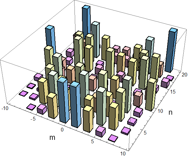
In the analysis reported above, the columns of the channel matrix $H$ correspond to excitations with all but one zero coefficients, i.e. each element transmitting as standalone. Now, we define a new channel matrix $\widetilde{H}$ in which the multiple inputs are coded as vortex modes instead of single elementary sources. In the simple case of a ring distribution of $N$ radiating elements, the $n$-th source excitation coefficient for the vortex mode with azimuthal index $m$ is given by:

It is an easy task to show that the vortex channel matrix $\widetilde{H}$ can be written as the product between the original matrix $H$ and the discrete Fourier transform (DFT) matrix $\Lambda$:

In (37), the DFT matrix can be written as $\Lambda_{jn}=\xi^{(m_{j})}_{n}$, where the $j$ index runs from 1 to $N$ and the following convention has been introduced:

It has been proven [14] that, in the simple case in which the elementary sources over the ring are replaced by ideal isotropic radiators, the set of excitations yielding the OAM modes directly provides the spectral basis for the corresponding channel matrix. However, elementary linearly polarized dipoles break the degenerate symmetry of the isotropic case and the interpretation of vortex modes as singular vectors of the channel matrix needs to be revisited. This circumstance can be brought to light by analyzing the spectral projection of the singular vectors of the channel matrix (33) on the OAM basis vectors (36), as reported in Fig. 7. It can be shown that one possible solution for restoring the lost circular symmetry is provided by the introduction of circularly polarized sources.

References

- [1] D. G. Grier, “A revolution in optical manipulation,” Nature, vol. 424, pp. 810–816, 2003.
- [2] M. Padgett and R. Bowman, “Tweezers with a twist,” Nature Photon., vol. 5, pp. 343–348, 2011.
- [3] M. Harwit, “Photon orbital angular momentum in astrophysics,” Astrophys. J., vol. 597, pp. 1266–1270, 2003.
- [4] F. Tamburini, B. Thidé, G. Molina-Terriza, and G. Anzolin, “Twisting of light around rotating black holes,” Nature Phys., vol. 7, pp. 195–197, 2011.
- [5] A. Mair, A. Vaziri, G. Weihs, and A. Zeilinger, “Entanglement of the orbital angular momentum states of photons,” Nature, vol. 412, pp. 313–316, 2001.
- [6] A. C. Dada, J. Leach, G. S. Buller, M. J. Padgett, and E. Andersson, “Experimental high-dimensional two-photon entanglement and violations of generalized Bell inequalities,” Nature Phys., vol. 7, pp. 677–680, 2011.
- [7] N. Bozinovic et al., “Terabit-scale orbital angular momentum mode division multiplexing in fibers,” Science, vol. 340, pp. 1545–1548, 2013.
- [8] M. Krenn et al., “Communication with spatially modulated light through turbulent air across Vienna,” New J. Phys., vol. 16, 2014.
- [9] G. Gibson et al., “Free-space information transfer using light beams carrying orbital angular momentum,” Opt. Express, vol. 12, pp. 5448–5456, 2004.
- [10] J. Wang et al., “Terabit free-space data transmission employing Orbital Angular Momentum multiplexing,” Nature Photon., vol. 6, pp. 488–496, 2012.
- [11] B. Thidé et al., “Utilization of photon orbital angular momentum in the low-frequency radio domain,” Phys. Rev. Lett., vol. 99, 2007.
- [12] F. Tamburini et al., “Encoding many channels on the same frequency through radio vorticity: first experimental test,” New J. Phys., vol. 14, 2012.
- [13] Y. Yan et al., “High-capacity millimetre-wave communications with orbital angular momentum multiplexing,” Nature Commun., vol. 5, 2014.
- [14] O. Edfors and A. J. Johansson, “Is orbital angular momentum (OAM) based radio communication an unexploited area?” IEEE Trans. Antennas Propag., vol. 60, pp. 1126–1131, 2012.
- [15] M. Tamagnone, C. Craeye, and J. Perruisseau-Carrier, “Comment on ‘Encoding many channels on the same frequency through radio vorticity: first experimental test’,” New J. Phys., vol. 14, 2012.
- [16] ——, “Comment on ‘Reply to Comment on “Encoding many channels on the same frequency through radio vorticity: first experimental test”’,” New J. Phys., vol. 15, 2013.
- [17] N. Zhao, X. Li, G. Li, and J. M. Kahn, “Capacity limits of spatially multiplexed free-space communication,” Nature Photon., vol. 9, pp. 822–826, 2015.
- [18] M. Chen, K. Dholakia, and M. Mazilu, “Is there an optimal basis to maximise optical information transfer?” Sci. Rep., vol. 6, 2016.
- [19] D. Slepian and H. O. Pollak, “Prolate spheroidal wave functions, Fourier analysis and uncertainty - I,” Bell Syst. Tech. J., vol. 40, pp. 43–63, 1961.
- [20] O. M. Bucci and G. Franceschetti, “On the spatial bandwidth of scattered fields,” IEEE Trans. Antennas Propag., vol. 35, pp. 1445–1455, 1987.
- [21] D. A. B. Miller, “Communicating with waves between volumes: evaluating orthogonal spatial channels and limits on coupling strengths,” Appl. Opt., vol. 39, pp. 1681–1699, 2000.
- [22] R. Piestun and D. A. B. Miller, “Electromagnetic degrees of freedom of an optical system,” J. Opt. Soc. Am. A, vol. 17, pp. 892–902, 2000.
- [23] J. Durnin, “Exact solutions for nondiffracting beams. I. The scalar theory,” J. Opt. Soc. Am. A, vol. 4, pp. 651–654, 1987.
- [24] J. D. Jackson, Classical Electrodynamics, 3rd ed. Wiley, New York, 1999.
- [25] R. L. Phillips and L. C. Andrews, “Spot size and divergence for Laguerre Gaussian beams of any order,” Appl. Opt., vol. 22, pp. 643–644, 1983.
- [26] D. K. Nguyen et al., “Antenna gain and link budget for waves carrying orbital angular momentum,” Radio Sci., vol. 50, pp. 1165–1175, 2015.
- [27] A. Vaziri, G. Weihs, and A. Zeilinger, “Superpositions of the orbital angular momentum for applications in quantum experiments,” J. Opt. B: Quant. Semiclass. Opt., vol. 4, pp. S47–S51, 2002.
- [28] R. Fickler et al., “Quantum entanglement of high angular momenta,” Science, vol. 338, pp. 640–643, 2012.
- [29] I. S. Gradshteyn and I. M. Ryzhik, Table of Integrals, Series and Products, 7th ed. Elsevier, New York, 2007.
- [30] E. T. Whittaker and G. N. Watson, A Course of Modern Analysis, 2nd ed. Cambridge Univ. Press, Cambridge, 1915.
- [31] R. Zambrini, L. C. Thomson, S. M. Barnett, and M. Padgett, “Momentum paradox in a vortex core,” J. Modern Opt., vol. 52, pp. 1135–1144, 2005.
- [32] M. Abramowitz and I. A. Stegun, Handbook of Mathematical Functions, with Formulas, Graphs, and Mathematical Tables, 10th ed. National Bureau of Standards, Washington, 1972.