$K$-sample omnibus non-proportional hazards tests based on right-censored data

Let $X$ be a one-dimensional non-negative random variable, $X\in\mathbb{R}^{+}$, and let $Y$ be a categorical variable indicating the group label. Under the $K$-sample hypotheses testing, the null hypothesis is $H_{0}:F_{1}(x)=\ldots=F_{K}(x)$ for all $x\in\mathbb{R}^{+}$, and the alternative is $H_{1}:F_{m}(x)\neq F_{k}(x)$ for some $1\leq m<k\leq K$ and some $x\in\mathbb{R}^{+}$, where $F_{k}$ is the cumulative distribution function of group $k$, $k=1,\ldots,K$. We assume that the sample spaces on which these $K$ distributions are defined, coincide.

$K$ random samples $\mathcal{A}_{1},\ldots,\mathcal{A}_{K}$ are drawn from the respective distributions $F_{1},\ldots,F_{K}$. Let $n_{k}$ be the total number of samples in group $k$, $k=1,\ldots,K$, and $n=\sum_{k=1}^{K}n_{k}$. Assume temporarily no censoring, and consider a pair of observations $X_{i}\in\mathcal{A}_{k}$ and $X_{j}$. Then, in the spirit of the HHG test (Heller et al. 2013), we consider the following partition induced by the pair $(i,j)$: $A_{11}(i,j)$ is the number of observations from group $k$ that the distance between the value of $X$ and $X_{i}$ is less than or equal to $|X_{i}-X_{j}|$; $A_{12}(i,j)$ is the number of observations outside group $k$ that the distance to $X_{i}$ is less than or equal to $|X_{i}-X_{j}|$; $A_{21}(i,j)$ is the number of observations from group $k$ that the distance to $X_{i}$ is larger than $|X_{i}-X_{j}|$; and $A_{22}(i,j)$ is the number of observations outside group $k$ that the distance to $X_{i}$ is larger than $|X_{i}-X_{j}|$.

Interestingly, with no censoring, the $A_{lr}$’s, $l,r=1,2$, can be expressed through the empirical cumulative distribution functions. For example, assume $X_{i}>X_{j}$ and $Y_{i}=Y_{j}=k$. Then,

	$\displaystyle A_{11}(i,j)$	$\displaystyle=$	$\displaystyle\sum_{r=1,r\neq i,j}^{n}I\{|X_{i}-X_{r}|\leq X_{i}-X_{j}\}I\{Y_{r}=k\}$
		$\displaystyle=$	$\displaystyle\sum_{r=1,r\neq i,j}^{n}I\{X_{j}\leq X_{r}\leq 2X_{i}-X_{j}\}I\{Y_{r}=k\}$
		$\displaystyle=$	$\displaystyle n_{k}\{\widehat{F}_{k}(2X_{i}-X_{j})-\widehat{F}_{k}(X_{j}^{-})\}-2\,,$

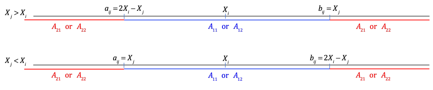
where $\widehat{F}_{k}(x)=n_{k}^{-1}\sum_{X_{l}\in\mathcal{A}_{k}}I(X_{l}\leq x)$ and $\widehat{F}_{k}(x^{-})=n_{k}^{-1}\sum_{X_{l}\in\mathcal{A}_{k}}I(X_{l}<x)$. The $-2$ above stands for excluding observations $i$ and $j$. In general, all observations with a distances to $X_{i}$ that is less than or equal to $|X_{i}-X_{j}|$ lie inside the interval $[a_{ij},b_{ij}]$, where $a_{ij}=\min(X_{j},2X_{i}-X_{j})$ and $b_{ij}=\max(X_{j},2X_{i}-X_{j})$, as illustrated in Figure 1.

In general, for $Y_{i}=k$, we get

	$\displaystyle A_{11}(i,j)$	$\displaystyle=$	$\displaystyle n_{k}\{\widehat{F}_{k}(b_{ij})-\widehat{F}_{k}(a_{ij}^{-})\}-1-I(Y_{i}=Y_{j})\,,$
	$\displaystyle A_{12}(i,j)$	$\displaystyle=$	$\displaystyle\sum_{m=1,m\neq k}^{K}n_{m}\big\{\widehat{F}_{m}(b_{ij})-\widehat{F}_{m}(a_{ij}^{-})\big\}-I(Y_{i}\neq Y_{j})\,,$
	$\displaystyle A_{21}(i,j)$	$\displaystyle=$	$\displaystyle n_{k}-A_{11}(i,j)-1-I(Y_{i}=Y_{j})\,,$
	$\displaystyle A_{22}(i,j)$	$\displaystyle=$	$\displaystyle\sum_{m=1,m\neq k}^{K}n_{m}-A_{12}(i,j)-I(Y_{i}\neq Y_{j})\,.$

For each pair $(i,j)$, a $2\times 2$ contingency table can be constructed with $A_{lr}(i,j)$ as the entry of cell $lr$, $l,r=1,2$, and a total sum of $n-2$. Under the null hypothesis of equal distributions, the probability of belonging to cell $lr$ equals the product of the marginal probabilities of the $l$th row and the $r$th column. Therefore, a summary statistic of a such contingency table can be based on either the Pearson chi-squared test statistic, or the log-likelihood ratio statistic. Since it is unknown which pair $(i,j)$ yields the best sample-space partition that provides the largest summary statistic, the final test statistic is defined as a sum over all possible $n(n-1)$ partitions induced by the data. A permutation-based $p$-value can be calculated, under random permutations of the group labels.

To introduce the right-censored data, let $C\in\mathbb{R}^{+}$ be a non-negative random variable indicating the censoring time. Assume that $X$ and $C$ are conditionally independent given $Y$. Define $T$ to be the observed time, namely $T=\min(X,C)$ and let $\Delta=I(X\leq C)$. Hence, the observed data consist of $K$ random samples that can be summarized by $(T_{i},\Delta_{i},Y_{i}),\ i=1,\ldots,n$. Note that the different groups may have different censoring distributions. With right-censored data, our proposed test requires special care in evaluating the $A_{r,l}$’s, $r,l=1,2$, by replacing the empirical distribution functions by their respective Kaplan–Meier (KM) estimators, as well as when applying a permutation test with unequal censoring distributions. Both issues are described in details below.

Let $\widetilde{F}_{k}$ be the KM estimator of the cumulative distribution function using all observations of group $k$. The KM estimator is defined only up to (and including) the last observed failure time. Define $\gamma_{k}$ to be the maximum time in which $\widetilde{F}_{k}$ can be used for the test statistic. If the largest observed time is a failure time, $\widetilde{F}_{k}(t)$ is known for the entire range of $t$. In this case, we define $\gamma_{k}$ to be the maximum possible value of $t$ required for the test, $2\max_{i=1,\ldots,n}\{T_{i}\}-\min_{i=1,\ldots,n}\{T_{i}\}$. However, in case of censoring after the largest failure time, the KM estimator beyond the largest observed failure time is undefined. We thus define the maximum time $\gamma_{k}$ to be the largest observed failure time. Namely,

$$\gamma_{k}=\left\{\begin{array}[]{ll}2\displaystyle\max_{i=1,\ldots,n}\{T_{i}\}-\displaystyle\min_{i=1,\ldots,n}\{T_{i}\}&\quad\mbox{if}\,\,\,\,\displaystyle\max_{i=1,\ldots,n}\{T_{i}\Delta_{i}I(Y_{i}=k)\}=\displaystyle\max_{i=1,\ldots,n}\{T_{i}I(Y_{i}=k)\}\\ \displaystyle\max_{i=1,\ldots,n}\{T_{i}\Delta_{i}I(Y_{i}=k)\}&\quad\mbox{if}\,\,\,\,\displaystyle\max_{i=1,\ldots,n}\{T_{i}\Delta_{i}I(Y_{i}=k)\}\neq\displaystyle\max_{i=1,\ldots,n}\{T_{i}I(Y_{i}=k)\}\end{array}\right.$$

Define $\gamma_{-k}$ to be the maximum time in which at least one of the other KM estimators, $\widetilde{F}_{m}$, $m=1,\ldots,K,m\neq k$, can be used for the test statistic, namely $\gamma_{-k}=\max_{m\neq k}\{\gamma_{m}\}$. Define $\tau_{k}$ to be the maximum time point the KM estimator is defined in group $k$ and in at least one more group, namely $\tau_{k}=\min\{\gamma_{k},\gamma_{-k}\}$. Then, for each pair of observed failure times $T_{i}\in\mathcal{A}_{k}$ and $T_{j}$ such that $j\neq i,\ \Delta_{i}=\Delta_{j}=1$ and $b_{ij}\leq\tau_{k}$, a $2\times 2$ contingency table is constructed. The following $A_{lr}^{*}(i,j),\ l,r=1,2$, are the corresponding expressions of $A_{lr}(i,j)$ obtained by replacing $\widehat{F}$ by $\widetilde{F}$, the KM estimators. In case $\gamma_{m}<b_{ij}$, the observations of group $m$ will not be included in the contingency table induced by the pair $(i,j)$. Namely, for $j\neq i,\ \Delta_{i}=\Delta_{j}=1,b_{ij}\leq\tau_{k}$ and $Y_{i}=k$,

	$\displaystyle A_{11}^{*}(i,j)$	$\displaystyle=$	$\displaystyle n_{k}\{\widetilde{F}_{k}(b_{ij})-\widetilde{F}_{k}(a_{ij}^{-})\}-1-I(Y_{i}=Y_{j})\,,$
	$\displaystyle A_{12}^{*}(i,j)$	$\displaystyle=$	$\displaystyle\sum_{m=1,m\neq k}^{K}n_{m}\big\{\widetilde{F}_{m}(b_{ij})-\widetilde{F}_{m}(a_{ij}^{-})\big\}I(\gamma_{m}\geq b_{ij})\ -I(Y_{i}\neq Y_{j})\,,$
	$\displaystyle A_{21}^{*}(i,j)$	$\displaystyle=$	$\displaystyle n_{k}-A_{11}^{*}(i,j)-1-I(Y_{i}=Y_{j})\,,$
	$\displaystyle A_{22}^{*}(i,j)$	$\displaystyle=$	$\displaystyle\sum_{m=1,m\neq k}^{K}n_{m}I(\gamma_{m}\geq b_{ij})-A_{12}^{*}(i,j)-I(Y_{i}\neq Y_{j})\,.$

Only pairs of observed failure times are used for the sample-space partitioning (i.e., $\Delta_{i}=\Delta_{j}=1$), while censored observations contribute in $\widetilde{F}_{k}$, $k=1,\ldots,K$. Denote by $n(i,j)$ the number of observations in all the groups included in the contingency table induced by $(i,j)$, namely $n(i,j)=\sum_{k=1}^{K}n_{k}I(\gamma_{k}\geq b_{ij})$. Let $S_{P}$ and $S_{LR}$ be the summary statistic of each contingency table, based on Pearson chi-squared test statistic

$$S_{P}(i,j)=\frac{\{n(i,j)-2\}\{A^{*}_{12}(i,j)A^{*}_{21}(i,j)-A^{*}_{11}(i,j)A^{*}_{22}(i,j)\}^{2}}{A^{*}_{1\cdot}(i,j)A^{*}_{2\cdot}(i,j)A^{*}_{\cdot 1}(i,j)A^{*}_{\cdot 2}(i,j)}\,,$$

and the log-likelihood ratio statistic,

$$S_{LR}(i,j)=2\sum_{m=1,2}\sum_{k=1,2}A^{*}_{mk}(i,j)\log\bigg[\frac{\{n(i,j)-2\}A^{*}_{kl}(i,j)}{A^{*}_{m\cdot}(i,j)A^{*}_{\cdot k}(i,j)}\bigg]\,,$$

respectively, where $A^{*}_{.k}(i,j)=\sum_{m=1,2}A^{*}_{mk}(i,j)$ and $A^{*}_{m.}(i,j)=\sum_{k=1,2}A^{*}_{mk}(i,j)$. In case of at least one zero margin in the contingency table, $S_{P}(i,j)=0$ and $S_{LR}(i,j)=0$. Denote by

$$N=\sum_{k=1}^{K}\sum_{i=1,T_{i}\in\mathcal{A}_{k}}^{n}\sum_{j=1,j\neq i}^{n}\Delta_{i}\Delta_{j}I(T_{j}\leq\tau_{k})I(b_{ij}\leq\tau_{k})$$

the total number of tables constructed from the data. Then, our proposed sample-space partition test statistic for equality of $K$ distributions based on right-censored data is defined by

$$Q=\frac{1}{N}\sum_{k=1}^{K}\sum_{i=1,T_{i}\in\mathcal{A}_{k}}^{n}\sum_{j=1,j\neq i}^{n}S(i,j)\Delta_{i}\Delta_{j}I(b_{ij}\leq\tau_{k})\,.$$

where $S(i,j)$ is either the test statistic $S_{P}(i,j)$ or $S_{LR}(i,j)$. In the case of no right censoring, the number of tables is solely determined by the number of observations. In right-censored data, the number of tables is random and determined also by the actual observed values due to the restrictions $\Delta_{i}=\Delta_{j}=1$ and $b_{ij}\leq\tau_{k}$. This issue is of high importance for the permutation stage of the test, as elaborated in the next subsection.

Allegedly, a permuted test can be done based on random permutations of the group labels. However, if the censoring distributions of the $K$ groups are different, such a permutation test is invalid, since a significant result can be yielded under the null due to differences in the censoring distributions. In order to generate random permutations that are independent of $Y$, we adopt the imputation approach suggested by Wang et al. 2010.

The main idea consists of randomly permuting the group labels, while for each observation assigned to a group different from the original one, a censoring time is imputed from the censoring distribution of the new assigned group. If the observation was originally censored, a survival time is also imputed, from the null survival distribution. Let $Y_{1}^{p},...,Y_{n}^{p}$ be a random permutation of the group labels. Define $(T_{i}^{p},\Delta_{i}^{p}),\ i=1,\ldots,n,$ by

$$(T_{i}^{p},\Delta_{i}^{p})=\left\{\begin{array}[]{ll}(T_{i},\Delta_{i})&\quad\mbox{if}\,\,\,\,Y_{i}^{p}=Y_{i}\\ (\widetilde{T}_{i},\widetilde{\Delta}_{i})&\quad\mbox{if}\,\,\,\,Y_{i}^{p}\neq Y_{i}\end{array}\,\,\,\,,\right.$$

where $\widetilde{T}_{i}=\min(\widetilde{X}_{i},\widetilde{C}_{i})$, $\widetilde{\Delta}_{i}=I(\widetilde{X}_{i}\leq\widetilde{C}_{i})$. Furthermore, $\widetilde{C}_{i}$ is sampled from the estimated censoring distribution of group $Y_{i}^{p}$, based on the KM estimator of the censoring distribution of group $Y_{i}^{p}$, by reversing the roles of event and censoring. The KM estimator, denoted by $\widehat{G}_{C,Y_{i}^{p}}$, is defined up to the largest observed censoring value of that group. Then, each observed censoring time is sampled with probability equals to the jump size of the respective KM estimator. In case $\widehat{G}_{C,Y_{i}^{p}}$ is incomplete, i.e., $\widehat{G}_{C,Y_{i}^{p}}\big[\max_{j=1,\ldots,n}\{T_{j}(1-\Delta_{j})I(Y_{j}=Y_{i}^{p})\}\big]>0$, the largest observed time, $\max_{j=1,\ldots,n}\{T_{j}(1-\Delta_{j})I(Y_{j}=Y_{i}^{p})\}$, is sampled with probability $\widehat{G}_{C,Y_{i}^{p}}\big[\max_{j=1,\ldots,n}\{T_{j}(1-\Delta_{j})I(Y_{j}=Y_{i}^{p})\}\big]$. $\widetilde{X}_{i}$ is defined by

$$\widetilde{X}_{i}=\left\{\begin{array}[]{ll}X_{i}&\quad\mbox{if}\,\,\,\,\Delta_{i}=1\\ X_{i}^{*}&\quad\mbox{if}\,\,\,\,\Delta_{i}=0\end{array}\,\,\,\,,\right.$$

where $X_{i}^{*}$ is sampled from an estimator of $\mbox{pr}(X_{i}>x|X_{i}>T_{i})$, the conditional distribution of $X$ under the null hypothesis. In practice, $\mbox{pr}(X_{i}>x|X_{i}>T_{i})$ is replaced by its KM estimator, using all observations from all groups that their observed time is larger than $T_{i}$. Denote this KM estimator by $\widehat{S}_{cond,T_{i}}$. The sampling based on $\widehat{S}_{cond,T_{i}}$ is done in the same fashion as in the above censoring sampling, but in case of incomplete distribution, the value $\max_{i=1,\ldots,n}(T_{i}\Delta_{i})+\varepsilon$ ($\varepsilon$ is any positive number) is sampled with probability $\widehat{S}_{cond,T_{i}}\{\max_{i=1,\ldots,n}(T_{i}\Delta_{i})\}$, and its respective event indicator is set to be $\Delta_{i}^{p}=0$, as there is no empirical evidence for the potential failure times beyond $\max_{i=1,\ldots,n}\{T_{i}\Delta_{i}\}$.

When performing a permutation test, the reported $p$-value can be viewed as an approximation of the true $p$-value, based on all possible permutations. In the above imputation-based permutation procedure, additional variability in a $p$-value is expected due to random imputations. To reduce this variability, multiple imputations can be used, such that for each random imputation, $B$ permutations are generated. Assume $M$ imputations are used. Then the $p$-value is defined as the fraction of the test statistics among the $MB$ test statistics that are at least as large as the observed test statistic $Q$.

In the following theorem it is argued that our proposed tests are consistent against all alternatives. The proof is presented in details in the Supplementary Materials.

Theorem: Let $X$ be a positive failure time random variable, either continuous or discrete, and $Y$ be a categorical random variable with $K$ categories. Let $\pi_{k}=\lim_{n\to\infty}n_{k}/n$, $k=1,\ldots,K$. Assume there are at least two cumulative distribution functions $F_{g}(x)$ and $F_{m}(x),\ g,m\in\{1,\ldots,K\}$, such that $F_{g}(x_{0})\neq F_{m}(x_{0})$ for some $x_{0}\in\mathbb{R}^{+}$, $\pi_{g}>0,\ \pi_{m}>0$, and the conditional censoring distributions are such that $\mbox{pr}(C>x_{0}|Y=g)>0$ and $\mbox{pr}(C>x_{0}|Y=m)>0$. Then, the imputation-based permutation test with the test statistic $Q$ is consistent, namely, the power of the test increases to $1$ as $n\to\infty$.

Table 1 provides the run time of the proposed tests of one dataset, $K=2$, under the null hypothesis, one imputation, and 1000 permutations, for different total sample sizes $n$ and $n_{1}=n_{2}=n/2$. These results were generated by a 6 years old Intel i7-3770 CPU 3.4 GHz, without paralleling with the different cores of the computer. The first two rows are for identical censoring distributions, and the last two are for different censoring distributions. Evidently, even with $n=1000$ observations and low censoring rates, the run time on such a simple computer is not longer than 3.5 minutes. We expect that an increase of the number of imputations and permutations will increase the run time in a linear fashion.

An extensive numerical study has performed to systematically examine the behavior of our proposed $K$-sample omnibus non-proportional hazards (KONP) tests under a wide range of alternatives, various sample sizes, and a wide range of censoring distributions, including unequal censoring distributions. The main part of the simulation study was dedicated to the popular 2-sample setting, but settings of $K=3,4,5$ were considered as well.

As competitors under the 2-sample setting, the following tests were included: the logrank test; Peto–Peto weighted logrank test (Peto and Peto 1972) that uses a weight function that is very close to the pooled KM estimator; Pepe–Fleming weighted KM test (Pepe and Fleming 1989) with geometric mean of the two KM censoring-distribution estimators as a weight function; and Yang–Prentice test, an adaptive weighted logrank test where the adaptive weights utilize the hazard ratio obtained by fitting the model of Yang and Prentice Yang and Prentice 2005. The tests of Uno et al. 2015 are invalid under unequal censoring distributions (as demonstrated below), and thus are not included in the following power comparisons.

Table 2 (main text) and tables A1 and A2 in Appendix, provide a comprehensive summary of the 17 non-proportional hazards scenarios and 7 proportional or close to proportional hazards functions, that were studied. For each scenario, the failure and censoring distributions are explicitly provided, and the survival functions of the two groups are plotted. A reference is provided indicating the source of each setting. In short, Scenario A shows differences at mid time points, but similarity in early and late times. Scenarios B–D show differences in early times. Scenario E is of equal survival functions at early times and of proportional hazards at mid and late times. Scenarios F and G are with crossing hazards. Scenario H is of a U-shape hazards ratio. Scenarios I, J and K are with crossing hazards, based on the following hazards-ratio model of Yang and Prentice 2005:

$$\mbox{HR}(t)=\frac{\lambda_{2}(t)}{\lambda_{1}(t)}=\frac{\theta_{1}\theta_{2}}{\theta_{1}+(\theta_{2}-\theta_{1})S_{1}(t)}\,,\,\,\,\,0<t<\tau_{0}\,,\,\,\,\,\theta_{1},\theta_{2}>0\,,$$

(1)

where $\tau_{0}=\sup\{t:S_{1}(t)>0\}$, $\lambda_{2}$ and $\lambda_{1}$ are the hazard functions of the two groups, and $S_{1}$ is the survival function of group $1$. Under Model (1), $\theta_{1}=\lim_{t\to 0}\mbox{HR}(t)$ and $\theta_{2}=\lim_{t\to\tau_{0}}\mbox{HR}(t)$. Also it is assumed that for a continuous function $S_{1}$, $\mbox{HR}(t)$ is a strong monotone function of $t$, i.e. $\mbox{sign}\{d\mbox{HR}(t)/dt\}$ is the same for all $t\in(0,\tau_{0})$. Scenarios I-1, I-2 and I-3 are with crossing hazards under Model (1). In I-1 the hazard functions cross earlier compared to I-2 and I-3. Scenarios J-1, J-2 and J-3 are with crossing hazards in which the strong monotonicity assumption is violated. In J-1 and J-2 the hazards are piece-wise proportional, and the hazard functions cross in mid time points. In Scenario J-3 the hazard ratio is a continuous function of $t$, and the hazards cross at a late time point. Under Scenarios K-1, K-2 and K-3 Model (1) is violated, but the strong monotonicity assumption of $\mbox{HR}(t)$ holds. In Scenarios K-1 and K-2 the hazards cross at early-mid times, and in Scenario K-3 at mid times.

For each scenario described above, four different censoring distributions were considered, two with equal and two with unequal censoring distributions. Under equal censoring distributions, the censoring distributions were taken to be similar to the corresponding referenced paper. Exponential distributions were used for all other scenarios, with approximately $25\%$ or $50\%$ censoring rates. Under unequal censoring distributions, the censoring distributions of Wang et al. 2010 were used (Table 2). The specific values of $(a,b,\theta_{1},\theta_{2})$ are provided in tables A1-A2. Under small differences, the censoring rates among the two groups are about $40\%$ and $55\%$, where $27\%$ and $55\%$ are the respective values under substantial differences. The various censoring settings are such that the power of a specific test under specific scenario is not necessarily increasing as the censoring rate decreases.

Each of the configurations was studied with $n=100,200,300$ or 400, $n_{1}=n_{2}$, and performances are summarized based on 2000 replications.

A smaller simulation study was done for $K>2$. As competitors, the logrank and Peto-Peto tests were included. For the null scenario $K=3,4,5$ were studied, and under Scenarios D and J-2, $K=3$ was examined. Various sample sizes and a wide range of censoring distributions were considered. A detailed description of these scenarios can be found in the Supplementary Materials.

Since the Yang–Prentice test is the strongest competitor in terms of power, for the $2$-sample setting, we highlight some of its properties. The Yang–Prentice test is based on Model (1), where the indices 1 and 2 indicate the control and treatment groups, respectively. Since this model is asymmetric in terms of $F_{1}$ and $F_{2}$, the test is not group-label invariant. By exchanging the group labels between ‘treatment’ and ‘control’, a different $p$-value would be provided. This property is unique to this test, and all other tests considered in this work are invariant to group labeling. Consequently, in applications with no clear link between the two groups to treatment/control status (e.g., comparing females versus males, or young versus old), it is unclear how the Yang–Prentice test should be applied.

In order to make the Yang–Prentice test invariant, we apply a permutation test based on the minimum $p$-value of the two labeling options. Specifically, let $PV_{1}$ and $PV_{2}$ be the $p$-values of the Yang–Prentice tests based on $(X_{i},\Delta_{i},Y_{i}),\ i=1,\ldots,n$, and $(X_{i},\Delta_{i},\widetilde{Y}_{i}),\ i=1,...,n$, respectively, where $Y_{i}\in\{1,2\}$ and $\widetilde{Y}_{i}=I(Y_{i}=2)+2I(Y_{i}=1)$. Then, the Yang–Prentice invariant test statistic is defined by $Q_{YP}=\min\{PV_{1},PV_{2}\}$. The $p$-value of the imputation-based permutation test, based on the statistic $Q_{YP}$, is the fraction of replicates of $Q_{YP}$ under random permutations of the data, as described in Section 2.3, that are at least as small as the observed test statistic. Since our work mainly focuses on invariant tests, we report and discuss in the main text the performance of the Yang–Prentice invariant test. The results of the original Yang-Prentice test, with the two possible options of labeling for treatment and control, can be found in the Supplementary Materials.

The original Yang–Prentice test (implemented in the R package YPmodel) uses the asymptotic distribution of the test statistic under the null hypothesis. Often, its empirical size is greater than the nominal level, especially under small sample size (see the Supplementary Material). In a recent work of Yang 2019, which deals with interim monitoring using adaptive weighted log-rank test, the author suggests using the re-sampling method of Lin et al. 1993 instead of the original asymptotic approach (Yang and Prentice 2010), for improving the type I error rate. The method of Lin et al. 1993 is also based on asymptotic results. Alternatively, the imputation approach of Wang et al. 2010 works very well in very small sample sizes, and it does not require asymptotic distribution. To make the comparison between the methods consistently, we use the imputation approach for both, our proposed method and the invariant version of Yang-Prentice test.

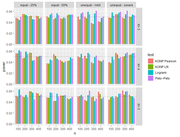
Figure 2 provides the empirical power of the tests under the null hypothesis, with equal and unequal censoring distributions. Evidently, under equal censoring distributions all the tests are valid, as the empirical size of the tests are reasonably close to the nominal value $0.05$. On the other hand, under the null hypothesis and unequal censoring distributions, the empirical sizes of Uno et al. tests are much higher than the nominal value 0.05. For example, under a sample size of $n=400$, and censoring rates of approximately $27\%$ and $55\%$, the empirical size of Uno et al. $V_{2}$ bona fide test is $0.099$; all the other Uno et al. tests’ sizes are even higher. The empirical sizes of all the other tests are reasonably close to their nominal value. Thus, Uno’s tests will not be considered in the rest of this simulation study.

Figure 3 summarizes the empirical power of the tests under settings generated by others, while Figure 4 is based on scenarios generated by us. As expected, the power of each test increases with the sample size. In some scenarios the power of the tests increases as the censoring rate increases, since in these settings the non-censored data are centered mainly at the parts of the hazards which are closer to proportionality and the censored data are mainly located at the non-proportionality area of the hazards. For example, in Scenario I-3 with $n=400$, as the censoring rate increases from about $25\%$ to about $50\%$, the power of Peto–Peto increases by $0.159$, Yang–Prentice by $0.2$, Pepe–Fleming by $0.218$, and logrank by $0.4$. The power increase in our KONP tests is much smaller, 0.012 and 0.009.

Evidently, our KONP tests are often more powerful compared to all other tests. These includes scenarios A, C, D, E, F, J-1, J-2, J-3, I-1, K-1, K-2, K-3. The superiority of KONP over Yang-Prentice under F and I-1 is surprising, since these scenarios follow their Model (1). For example, with $n=400$ and $25\%$ censoring rate, the empirical power is about $90\%$ for KONP tests and only $70\%$ for Yang–Prentice. In Scenario G (close to proportional hazards), which also follows Model (1), the results of Yang-Prentice and logrank are similar and often slightly better than KONP tests. In scenarios J-1 and J-2 our tests are substantially more powerful than all the competitors. For example, in Scenario J-2, $n=400$, and $25\%$ censoring rate, KONP tests with about $95\%$ power, while the second most powerful test is Yang–Prentice with a power of $48\%$.

In scenarios G, I-2 and in some of the censoring rates in I-3, the Peto–Peto and Pepe–Fleming tests tend to be with the highest power. In contrast, in many of the scenarios in which the survival functions cross, their power are much lower than our tests. For example, in Scenario K-1, $n=400$, and $25\%$ censoring rate, the power of KONP is $89\%$, while Pepe–Fleming power is $42\%$ and Peto–Peto is $5\%$.

To conclude, for the $2$-sample setting, in most of the non-proportional hazards settings, our proposed KONP tests tend to be more powerful than the other tests, and the differences between $S_{P}$ and $S_{LR}$ are very small, if any.

Results of settings with $K>2$ can be found in Table S1 and Figure S1 of the Supplementary Material. Based on these results we conclude that all the tests are valid, as the empirical size of the tests are reasonably close to $0.05$. For $K=3$ and scenarios D and J-2, we see similar results to those shown with $K=2$, as KONP tests are often much more powerful than the logrank and Peto–Peto test. For example, for scenario D with $n=200$ and $25\%$ censoring rates in all the three groups, the powers of KONP tests are approximately $92\%$, while of Peto–Peto is $49\%$, and of logrank is $18\%$.

Figure 5 summarizes the power of the 2-sample tests under proportional hazards or close to proportionality. Under these settings the logrank test is often with the highest power among the invariant tests, as expected. The invariant version of Yang–Prentice test is similar to the logrank test, and the proposed KONP tests, sometimes, have less power.

Figures 3 and 4 of the main text and Table S2 of the Supplementary Material indicate that under the non-proportional hazards scenarios and among the invariant tests, usually the proposed KONP tests are with the largest power. Under proportional hazards or close to proportionality, usually the logrank test is with the largest power among the invariant tests. The invariant version of Yang–Prentice test is similar to the logrank test under proportional hazards settings, since their model contains the proportional hazards model ($\theta_{1}=\theta_{2}$).

In case one is interested in a robust powerful test under non-proportional or proportional hazards, the principle of minimum p-value could be adopted based on the elegant Cauchy-combination test of Liu and Xie 2019, which is similar to the test based on the minimum $p$-value. Denote the $p$-values of our KONP tests by $p\mbox{-value}_{P}$ and $p\mbox{-value}_{LR}$, respectively, and the $p$-value of the logrank test by $p\mbox{-value}_{lgrnk}$. Then, based on Liu and Xie 2019 we define a new test statistic

$$Cau=[\tan\{(0.5-p\mbox{-value}_{P})\pi\}]/3+[\tan\{(0.5-p\mbox{-value}_{LR})\pi\}]/3+[\tan\{(0.5-p\mbox{-value}_{lgrnk})\pi\}]/3\,,$$

and its $p$-value is

$$p\mbox{-value}_{Cau}=0.5-(\arctan Cau)/\pi\,.$$

The candidate tests to be included in ${Cau}$ are powerful tests under non-proportional (i.e. KONP tests) or proportional hazards (i.e. logrank test and the invariant version of Yang–Prentice test). Due to the similarity in power performances between the logrank test and the invariant version of Yang–Prentice test, under proportional or close to proportional hazards, and due to the high computational burden of Yang–Prentice invariant test, only the logrank test is included.

Figure S3 of the Supplementary Materials provides the empirical Type-I error of the two KONP tests, the logrank test and the robust $Cau$ test. Evidently, the size of the tests are reasonably close to 0.05. Figures S4-S5 of the Supplementary Materials summarize the empirical power, based on 1000 replications, of the two KONP tests, the logrank test and the test statistic $Cau$. Often, the $Cau$ test loses some power comparing to the largest power among KONP and logrank, but the loss is relatively small. Table S4 of the Supplementary Materials provides the power values of these tests under all the studied alternatives, along with two additional combined test: the test of Lee Lee 2007 which is based on the maximum of two weighted logrank test statistics; and the MaxCombo test Lin et al. 2019 which is based on the maximum of the logrank and three weighted logrank test statistics. (See Supplementary Materials for details.) Lee and MaxCombo tests perform very similarly. In general, our $Cau$ test outperforms Lee and the MaxCombo tests, in terms of power, in all the sub-scenarios (i.e., various sample size and censoring patterns) of type B, C, H, J-1, and J-2; and in some of the sub-scenarios of A, F, I-1, I-2, I-3, K-1, K-2, K-3, and P. All of these are non-proportional hazards scenarios. Under proportional hazards or close to proportionality, i.e., settings L, M, N O, P and Q, Lee’s test or MaxCombo outperform $Cau$. Interestingly, the cases where Lee or MaxCombo tests are with higher power than $Cau$, the power loss by using $Cau$ is relatively small; while this is not always the case when $Cau$ outperforms Lee or MaxCombo. For example, under Setting B with $n=200$, the power of $Cau$ equals 0.919 while the power values of Lee and MaxCombo are 0.499 and 0.450, respectively.

Our R package KONPsurv (Schlesinger and Gorfine 2019) applies the above robust test $Cau$ as well.

The Gastrointestinal Tumor Study Group (Schein and Group 1982) compared chemotherapy with combined chemotherapy and radiation therapy, in the treatment of locally unresectable gastric cancer. This dataset was used in Yang and Prentice 2010 to demonstrate the utility of their test. Each treatment arm had 45 patients, and two observations of the chemotherapy group and six of the combination group were censored. The primary outcome measure was time to death. The KM survival curves of time to death, in each treatment group are provided in Figure 6. To apply the Yang–Prentice test, we considered chemotherapy as the control group and chemotherapy plus radiation therapy as the treatment group, which is named Yang–Prentice 1. The Yang–Prentice test with reversed group labeling is denoted by Yang–Prentice 2. Table 3 shows the $p$-values of testing for equality of the survival curves of time to death, of the two treatment groups, against a two-sided alternative, with each of the tests considered in the simulation study. For our tests and the Yang-Prentice invariant test, $10$ imputations and $10^{4}$ permutations for each imputation, were used. Evidently, the smallest $p$-values are observed under our proposed KONP tests and the Cauchy-combination test $Cau$.

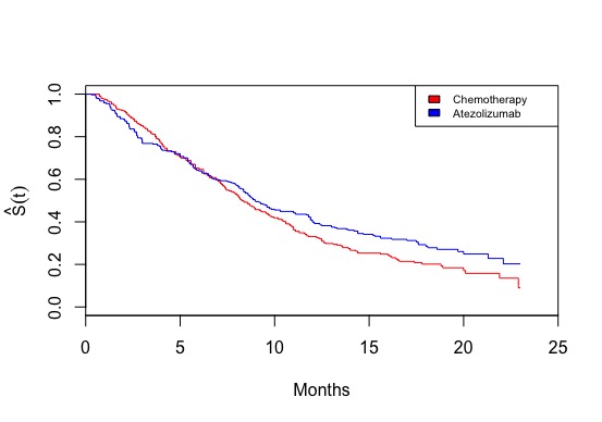
Few options exist for patients with locally advanced or metastatic urothelial carcinoma after progression with platinum-based chemotherapy. Powel et al. Powel et al. 2018 aimed to assess the safety and efficacy of atezolizumab versus chemotherapy in this patient population. Their study consists of a multi-center, open-label, phase 3 randomised controlled trial conducted at 217 academic medical centers and community oncology practices mainly in Europe, North America, and the Asia-Pacific region. The primary endpoint was overall survival. Figure S3 of the Supplementary Material of Powel et al. 2018 provides the overall survival KM curves of atezolizumab versus chemotherapy based on 316 and 309 patients, respectively. Although the detailed survival data are unavailable, inspired by Roychoudhury et al. 2019 we used Guyot et al. Guyot et al. 2012 algorithm that maps from digitised curves back to KM data, by finding numerical solutions to the inverted KM equations, using available information on number of events and numbers at risk. The DigitizeIt software was used for reading the coordinates of the KM curves from the published graph. Figure 7 provides the KM curves by treatment arm, and the last column of Table 3 shows the $p$-values of testing for equality of the survival curves of time to death against a two-sided alternative. Evidently, the smallest $p$-values are observed under our proposed KONP tests and the second best is the test of Lee. Our Cauchy combined test also performs robustly.

References

- Yang and Prentice (2010) Yang S and Prentice RL. Improved logrank-type tests for survival data using adaptive weights. Biometrics, 66(1):30–38, 2010.
- Peto and Peto (1972) Peto R and Peto J. Asymptotically efficient rank invariant test procedures. Journal of the Royal Statistical Society. Series A, pages 185–207, 1972.
- Pepe and Fleming (1989) Pepe MS and Fleming TR. Weighted Kaplan–Meier statistics: a class of distance tests for censored survival data. Biometrics, pages 497–507, 1989.
- Pepe and Fleming (1991) Pepe MS and Fleming TR. Weighted Kaplan–Meier statistics: Large sample and optimality considerations. Journal of the Royal Statistical Society. Series B, pages 341–352, 1991.
- Yang and Prentice (2005) Yang S and Prentice RL. Semiparametric analysis of short-term and long-term hazard ratios with two-sample survival data. Biometrika, 92(1):1–17, 2005.
- Darling (1957) Darling DA. The Kolmogorov–Smirnov, Cramer–von Mises tests. Annals of Mathematical Statistics, 28(4):823–838, 1957.
- Pettitt (1976) Pettitt AN. A two-sample Anderson–Darling rank statistic. Biometrika, 63(1):161–168, 1976.
- Scholz and Stephens (1987) Scholz FW and Stephens MA. -sample Anderson–Darling tests. Journal of the American Statistical Association, 82(399):918–924, 1987.
- Thas and Ottoy (2004) Thas O and Ottoy JP. An extension of the Anderson–Darling -sample test to arbitrary sample space partition sizes. Journal of Statistical Computation and Simulation, 74(9):651–665, 2004.
- Heller et al. (2013) Heller R, Heller Y, and Gorfine M. A consistent multivariate test of association based on ranks of distances. Biometrika, 100(2):503–510, 2013.
- Heller et al. (2016) Heller R, Heller Y, Kaufman S, Brill B, and Gorfine M. Consistent distribution-free -sample and independence tests for univariate random variables. Journal of Machine Learning Research, 17(1):978–1031, 2016.
- Wang et al. (2010) Wang R, Lagakos SW, and Gray RJ. Testing and interval estimation for two-sample survival comparisons with small sample sizes and unequal censoring. Biostatistics, 11(4):676–692, 2010.
- Uno et al. (2015) Uno H, Tian L, Claggett B, and Wei LJ. A versatile test for equality of two survival functions based on weighted differences of Kaplan–Meier curves. Statistics in medicine, 34(28):3680–3695, 2015.
- Yang (2019) Yang S. Interim monitoring using the adaptively weighted log-rank test in clinical trials for survival outcomes. Statistics in medicine, 38(4):601–612, 2019.
- Lin et al. (1993) Lin DY, Wei LJ, and Ying Z. Checking the cox model with cumulative sums of martingale-based residuals. Biometrika, 80(3):557–572, 1993.
- Liu and Xie (2019) Liu Y and Xie J. Cauchy combination test: a powerful test with analytic p-value calculation under arbitrary dependency structures. Journal of the American Statistical Association 1-18, 2019.
- Lee (2007) Seung-Hwan L. On the versatility of the combination of the weighted log-rank statistics. Computational Statistics & Data Analysis , 51(12), 6557–6564, 2007.
- Lin et al. (2019) Lin RS, et al. Alternative Analysis Methods for Time to Event Endpoints under Non-proportional Hazards: A Comparative Analysis. arXiv preprint arXiv:1909.09467, 2019.
- Schlesinger and Gorfine (2019) Schlesinger M and Gorfine M. Konp tests: Powerful k-sample tests for right-censored data. 2019. R package version 1.0.1.
- Schein and Group (1982) Schein PS and Gastrointestinal Tumor Study Group. A comparison of combination chemotherapy and combined modality therapy for locally advanced gastric carcinoma. Cancer, 49(9):1771–1777, 1982.
- Powel et al. (2018) Powles T et al. Atezolizumab versus chemotherapy in patients with platinum-treated locally advanced or metastatic urothelial carcinoma (IMvigor211): a multicentre, open-label, phase 3 randomised controlled trial. The Lancet 391: 748–757, 2018.
- Roychoudhury et al. (2019) Roychoudhury S et al. Robust Design and Analysis of Clinical Trials With Non-proportional Hazards: A Straw Man Guidance from a Cross-pharma Working Group. arXiv preprint arXiv:1908.07112, 2019.
- Guyot et al. (2012) Guyot P, Ades AE, Ouwens MJ, and Welton NJ. Enhanced secondary analysis of survival data: reconstructing the data from published Kaplan-Meier survival curves. BMC medical research methodology, (12):9, 2012.
6 Appendix
6.1 Detailed Description of the Simulation Settings