Asteroid pairs: a complex picture
Abstract
We studied a sample of 93 asteroid pairs, i.e., pairs of genetically related asteroids that are on highly similar heliocentric orbits. We estimated times elapsed since separation of pair members (i.e., pair age) that are between yr and a few yr. With photometric observations, we derived the rotation periods for all the primaries (i.e., the larger members of asteroid pairs) and a sample of secondaries (the smaller pair members). We derived the absolute magnitude differences of the studied asteroid pairs that provide their mass ratios . For a part of the studied pairs, we refined their WISE geometric albedos and collected or estimated their taxonomic classifications. For 17 asteroid pairs, we also determined their pole positions. In two pairs where we obtained the spin poles for both pair components, we saw the same sense of rotation for both components and constrained the angles between their original spin vectors at the time of their separation. We found that the primaries of 13 asteroid pairs in our sample are actually binary or triple systems, i.e., they have one or two bound, orbiting secondaries (satellites). As a by-product, we found also 3 new young asteroid clusters (each of them consisting of three known asteroids on highly similar heliocentric orbits). We compared the obtained asteroid pair data with theoretical predictions and discussed their implications. We found that 86 of the 93 studied asteroid pairs follow the trend of primary rotation period vs mass ratio that was found by Pravec et al. (2010). Of the 7 outliers, 3 appear insignificant (may be due to our uncertain or incomplete knowledge of the three pairs), but 4 are high mass ratio pairs that were unpredicted by the theory of asteroid pair formation by rotational fission. We discuss a (remotely) possible way that they could be created by rotational fission of flattened parent bodies followed by re-shaping of the formed components. The 13 asteroid pairs with binary primaries are particularly interesting systems that place important constraints on formation and evolution of asteroid pairs. We present two hypotheses for their formation: The asteroid pairs having both bound and unbound secondaries could be “failed asteroid clusters”, or they could be formed by a cascade primary spin fission process. Further studies are needed to reveal which of these two hypotheses for formation of the paired binary systems is real.
Keywords:
Asteroids, dynamics; Asteroids, rotation; Photometry, , , , , , , , , , , , , , , , , , , , , , , , , , , , , , , , , , , , , , , , , , , , , , ,
Proposed running head: Asteroid pairs complex
Editorial correspondence to:
Dr. Petr Pravec
Astronomical Institute AS CR
Fričova 1
Ondřejov
CZ-25165
Czech Republic
Phone: 00420-323-620352
Fax: 00420-323-620263
E-mail address: petr.pravec@asu.cas.cz
1 Introduction
In the main belt of asteroids, there exist pairs of asteroids that are on highly similar heliocentric orbits. They were discovered by Vokrouhlický and Nesvorný (2008) who showed that the asteroid pairs cannot be random coincidences of unrelated asteroids from the local asteroid population, but most of them must be genetically related pairs. They proposed 60 such asteroid pairs. Pravec and Vokrouhlický (2009) developed a statistical asteroid pair identification procedure and they found 73 statistically significant pairs (most of them have been confirmed by backward orbit integrations; see Section 2). Pravec et al. (2010) studied a sample of 32 asteroid pairs and found a correlation between the rotation frequencies of asteroid pair primaries11 1 We call ‘primary’ and ‘secondary’, respectively, the larger and the smaller member of an asteroid pair. and the asteroid pair mass ratios. Following the theory by Scheeres (2007), they found the correlation to be an evidence for formation of asteroid pairs by rotational fission.
A number of dynamical and physical studies of asteroid pairs were published since then. Vokrouhlický and Nesvorný (2009) and Vokrouhlický et al. (2011, 2017) studied the young asteroid pair of (6070) Rheinland and (54827) Kurpfalz.22 2 Hereafter we for short designate asteroid pairs with the primary and secondary asteroid numbers (or principal designations), e.g., 6070–54827 for the pair of (6070) Rheinland and (54827) Kurpfalz. They determined its age of kyr and found that the spin vectors of the two asteroids are both retrograde, but they were not colinear but tilted by at the time of separation. Žižka et al. (2016) studied asteroid pair 87887–415992 and found it to have a probable age of kyr, that is probably the youngest one of known asteroid pairs. Vokrouhlický (2009) found that the triple asteroid (3749) Balam is paired with asteroid 2009 BR60, which was the first known case of such complex system with both bound and unbound secondaries. Polishook (2014a) found that the members of pair 2110–44612 have the same sense of rotation (retrograde), as expected for an asteroid pair formed by rotational fission. Pravec et al. (2018) studied 13 young asteroid clusters (i.e., groups of three or more genetically related asteroids on highly similar heliocentric orbits) and found that the properties of 11 of them are consistent with the rotational fission formation process, linking them to asteroid pairs.
Spectral or color observations of paired asteroids33 3 We use the term ‘paired asteroid’ as a synonym for ‘member of an asteroid pair’. were done by Moskovitz (2012), Duddy et al. (2012, 2013), Wolters et al. (2014) and Polishook et al. (2014a). They found that the pairs belong to a variety of taxonomic classes, indicating that the asteroid structure and not their composition, is the main property that enabled their fission. They also found that in most asteroid pairs, the two components have the same or similar spectra and colors, consistent with same composition of both components as expected for the secondary formed by fission from the primary. Some silicate pairs, belonging to the S-complex, present subtle spectral/color differences between the primary and secondary, which they suggested could be due to different degrees of “space weathering” of the surfaces of the pair members. As they found no large-scale spectral non-uniformity on the surfaces of young asteroid pairs, Polishook et al. (2014b) suggested that the rotational fission was followed by a spread of dust that covered the primary body uniformly.
Being motivated by the progress in our knowledge and understanding of asteroid pairs as briefly outlined above, we underwent a thorough photometric study of a sample of nearly 100 asteroid pairs. This study has not only enlarged the sample of studied asteroid pairs by nearly a factor of 3, but it also went to smaller asteroid sizes than before, extending our knowledge of asteroid pair properties to sizes about 1 km where we start seeing new features in the asteroid pair population. And we also performed observations within this survey thoroughly so that to be able to resolve also potential binary nature of studied asteroids. We outline our results in this paper.
2 Pair identification and age estimation
We identified candidate asteroid pairs by analyzing the distribution of asteroid distances in the five-dimensional space of mean orbital elements using the method of Pravec and Vokrouhlický (2009).44 4 Pravec and Vokrouhlický (2009) originally used osculating orbital elements, but later we amended the method with the use of mean elements, following suggestion by D. Nesvorný (2010, personal communication; see also Rożek et al. 2011). See also an application of the method for asteroid clusters in Pravec et al. (2018). We took the mean elements from the AstDyS catalog webpage (Knežević et al. 2002, Knežević and Milani 2003). The distance () between two asteroid orbits was computed with a positive-definite quadratic form
| (1) |
where and are the mean motion and semimajor axis of either of the two asteroids and is the separation vector of their mean orbital elements. Following Zappalà et al. (1990) and Pravec and Vokrouhlický (2009), we used , and . The distance between two asteroid orbits is an approximate gauge for the relative velocity of the asteroids at close encounter (see Rożek et al. 2011 for explicit tests and a comparison with other metric functions used in meteoritics). For most asteroid pairs, it is in the range from a few to a few 10 m/s.
To confirm the pair membership suggested by the asteroid distances in the space of mean orbital elements, we integrated a set of geometric clones (1000 clones for each asteroid) with the Yarkovsky effect acting on each clone differently. The Yarkovsky effect was represented using a fake transverse acceleration acting on the clone with a magnitude providing secular change in semimajor axis (see Farnocchia et al., 2013). It was chosen from the range , where was estimated from the asteroid size (see Vokrouhlický, 1999). These limit values for the semimajor axis drift rate correspond to bodies with zero obliquity, for which the diurnal variant of the effect is optimized, and the diurnal thermal parameter equal to the square root of two, for which the magnitude of the Yarkovsky effect is maximal (see, e.g., Vokrouhlický, 1999). The goal of our backward orbital integrations was to find low relative-velocity close encounters between the clones of the members of a tested pair. We chose following limits on the physical distance and relative velocity between the clones and , where and are the radius of the Hill sphere and the surface escape velocity, respectively, of the primary body. The narrower limits were used for better converging clones (e.g., younger ones, or those in non-chaotic zones of the main asteroid belt), while the loosened limits were typically used for pairs with the orbits affected by some orbital chaoticity. The radius of the Hill sphere was estimated as , where is the semi-major axis of the primary’s heliocentric orbit, is its diameter, is its bulk density (assumed 2 g/cm3), is the gravitational constant and is the gravitational parameter of the Sun. The escape velocity was estimated as (both formulas from Pravec et al., 2010, Supplementary Information).
For numerical integration we used the fast and accurate implementation of a Wisdom-Holman symplectic integrator WHFast (Rein and Tamayo, 2015) from the REBOUND package (Rein and Liu, 2012). We implemented the Yarkovsky effect into the code following Nesvorný and Vokrouhlický (2006). We included gravitational attraction of the Sun, the 8 major planets, two dwarf planets Pluto and Ceres and two large asteroids Vesta and Pallas. We chose the time-step to be six hours, this allows us to detect close and fast encounters with massive bodies in our simulation. The geometric clones were created in the six-dimensional space of equinoctial elements E using the probability distribution , where is the difference with respect to the best-fit orbital values and is the normal matrix of the orbital solution downloaded from AstDyS website at the initial epoch MJD 58000 (Milani and Groncchi, 2010). Each geometric clone was given a random value of from the range .
For each pair, we estimated a time since separation of the secondary from the primary (designated ) from the distribution of the calculated past times of close and slow encounters between their clones. With the output frequency of 10 days we checked all the clone combinations () between the primary and the secondary and for each we found their minimum distance and relative velocity at their encounter. Encounters satisfying the chosen distance and velocity limits (see above) were counted and their time histogram was used for estimating for given tested pair. The histograms for individual asteroid pairs are shown in Section 3 or in the Electronic Supplementary Information. The bin widths in the histograms are 10 or 20 kyr for the past time axis spanning to or kyr, respectively. As the distributions of are non-Gaussian and often strongly asymmetric, we used the median (i.e., the 50th percentile) value of the distribution as a nominal estimate for the time of separation of the members of given pair (i.e., the pair age). For an uncertainty (error bar) of the separation time, we adopted the 5th and the 95th percentile of the distribution for the lower and upper limit on the separation time, respectively.
3 Asteroid pair properties
We collected available lightcurve photometric data and run new photometric observations for all the primaries and some secondaries of our sample of 93 asteroid pairs. We used our standard photometric observational and reduction techniques that we describe in Electronic Supplementary Information. The obtained data were analysed using the methods described in Pravec et al. (2006) that provided rotation periods of the studied paired asteroids and revealed the binary nature of several of them. For paired asteroids with sufficient data, we derived their spin vectors and constructed their convex shape models using the technique of Kaasalainen et al. (2001), with confidence ranges estimated as in Vokrouhlický et al. (2011). For most primaries and some secondaries, we also derived their accurate absolute magnitudes, from which we calculated their values55 5 We designate quantities belonging to the primary and secondary with the indices ‘1’ and ‘2’, respectively. and propagated their uncertainties for pairs where we had the accurate absolute magnitudes for both members of a given pair. However, the absolute magnitudes for some primaries and many secondaries for which we did not obtain accurate values were taken from the MPC catalog66 6 http://www.minorplanetcenter.org/iau/MPCORB.html.. The uncertainties of in such cases were assumed to be (see Pravec et al., 2012a, for analysis of the uncertainties of absolute magnitudes reported in asteroid orbit catalogs). The asteroid pair mass ratio is estimated from its value with
| (2) |
Where available, we took the diameters and geometric albedos of studied asteroids from their WISE observations (Masiero et al. 2011) and refined them using our accurate values using the method described in Pravec et al. (2012b). For three asteroids, we derived their diameters and geometric albedos from thermophysical modeling (Appendix A). For a sample of paired asteroids, we also measured their colors with Sloan Digital Sky Survey (SDSS) filters or took their SDSS color measurements from the SDSS Moving Object Catalog (Ivezić et al. 2001), and used them to estimate their taxonomic classifications. SDSS photometric data for individual objects were obtained in sequences employing the g’r’i’z’ filters. The mean color indices and the mean for individual measured asteroids are given in Suppl. Table 2. Taxonomic classification was achieved by down-sampling the resolution of the spectral envelopes in the Bus taxonomic system (Bus and Binzel, 2002) to the SDSS filter set and then minimizing the RMS residual between the photometric data and the taxonomic envelopes. In some cases the data were equivalently well fit with more than one taxonomic type, in which case we present two possible assignments. For several paired asteroids, we also collected published taxonomic classification from spectral data.
The data for the studied asteroid pairs are presented in Tables 3 to 6. In Table 3, for each studied asteroid pair, we give the distance of its members in the space of mean orbital elements (), its age estimated from the backward orbital integrations of the pair members, the primary and secondary absolute magnitudes (), its , the primary diameter () derived from the WISE observations (if given to a tenth of km) or estimated assuming the mean geometric albedo of its derived or estimated taxonomic type (if rounded to 1 km), the primary and secondary rotation periods and mean observed lightcurve amplitudes (), and a number of observed satellites (bound secondaries) of the primary (Sat.1). In the last column, we note subsections and/or tables where more data and information are given for a given asteroid pair. For most asteroid pairs, we also give further information in Electronic Supplementary Information.
In Table 4, we give the geometric albedos () of the pair primaries that we refined from the WISE data using our accurate absolute magnitudes or from our thermophysical modeling presented in Appendix A. In columns Taxon.1 and Taxon.2, we report the primary and secondary taxonomic classifications. The 6th and 7th columns are their color indices in the Johnson-Cousins VR photometric system that we obtained as by-product of our lightcurve observations or derived from their Sloan colors using the formula (Jester et al., 2005). In the last column, we mention where more information on the reported quantities is given.
In Table 5, we report the ecliptic coordinates (in equinox J2000) of the spin poles of several paired asteroids for which we derived their spin vectors or the orbit poles of four binary systems among asteroid pair primaries. The sidereal periods of the paired asteroids with derived spin vectors are given in the or columns in Table 3. Their convex shape models or information about the binary systems are given in subsections mentioned in the last column.
In Table 6, we report the best estimates (nominal values) for several parameters of the binary systems among asteroid pairs. Uncertainties of the values are given in the text or they are available in the binary asteroid parameters tables at http://www.asu.cas.cz/asteroid/binastdata.htm (update of the original tables from Pravec and Harris, 2007). We give the diameter of the primary (main body) of the binary system , the mean diameter ratio between the unbound secondary and the primary , the mean diameter ratio between the bound secondary (satellite) and the primary , the ratio of the major semiaxis of the binary system to the primary’s mean diameter , the constrained or assumed eccentricity (3- ranges or upper limits on the eccentricity are given, or zero eccentricity is assumed in cases where the available data is consistent with circular orbit of the satellite but we did not obtain a full model of the secondary’s orbit yet), the primary and secondary rotation periods and , the orbital period , the normalized total angular momentum (see Pravec and Harris, 2007, for its definition), the observed lightcurve amplitudes of the primary and the secondary and , measured at mean solar phase SolPh, and the estimated primary and secondary equatorial axes ratios and . In the last column, we note the subsections on the paired binary systems where more information is given.
In following subsections, we present the results for selected individual asteroid pairs that are particularly interesting in certain points.
3.1 (1741) Giclas and (258640) 2002 ER36
This is a secure asteroid pair with an estimated age about 200 kyr (Fig. 1). From spectral observations of the primary, Polishook et al. (2014a) derived that it is S/Sq type. We obtained its color index as the weighted mean of our measured and the value by Slivan et al. (2008). We derived its prograde spin pole (with two mirror solutions in longitude, see Table 5). The best-fit convex shape models for the two pole solutions are shown in Figs. 2 and 3. From our thermophysical modeling, we derived its effective volume-equivalent diameter and geometric albedo (Appendix A). On the nights 2015-06-05.6, -06.6, and 2018-01-25.2, we detected brightness attenuations with depths 0.06–0.07 mag that suggest a presence of satellite (bound secondary). This suspicion of binary nature of (1741) Giclas needs to be confirmed with thorough observations in the future.


3.2 (2110) Moore-Sitterly and (44612) 1999 RP27
This is a secure asteroid pair with an estimated age about 2 Myr (Fig. 4). From their spectral observations, Polishook et al. (2014a) derived S and Sq/Q types for the primary and secondary, respectively. Their color indices are (Moskovitz 2012) and (our measurement). Using our derived mean absolute magnitude, we refined the WISE data (Masiero et al. 2011) for the secondary (44612) and obtained km and . For both asteroids, we derived their retrograde spin vectors (with two mirror solutions in longitude, see Table 5), in agreement with their earlier models by Polishook (2014a). The best-fit convex shape models for the two pole solutions for both the primary and the secondary are shown in Figs. 5 to 8. Though the best-fit pole positions for the two asteroids are nearly 90∘ distant in longitude, their 3- pole uncertainty areas overlap, see their plots in the Electronic Supplementary Information. Finally, from our thermophysical modeling, we derived the primary’s volume-equivalent diameter and geometric albedo (Appendix A).


3.3 (3749) Balam and (312497) 2009 BR60
This is a secure asteroid pair with an estimated age about 400 kyr (Fig. 9). The primary (3749) Balam has two satellites. The outer satellite was discovered by Merline et al. (2002) and the inner satellite was discovered by Marchis et al. (2008). Vokrouhlický (2009) identified the unbound secondary (312497). For the outer satellite of the primary, Vachier et al. (2012) derived a set of possible orbital solutions with the semi-major axis ranging from 189 to 298 km, orbital period from 1306 to 3899 h, and eccentricity from 0.35 to 0.77. From the magnitude difference between their images of the outer satellite and the primary plus inner satellite (which was not resolved in their images) reported by Merline et al. (2002) and applying a correction for the presence of the unresolved inner satellite, we estimate the size ratio for the outer satellite. From the observed total mutual events between the inner satellite and the primary, we derived its size ratio . Its orbital period is h (Marchis et al. 2008) and it appears synchronous, i.e., its rotational period appears equal to the orbital period. Its orbit is slightly eccentric, –0.08 (3- range; Scheirich et al., in preparation). Refining the WISE thermal measurements (Masiero et al. 2011) with our accurately determined mean absolute magnitude of the whole system of Balam , we obtained the effective diameter km and geometric albedo . Correcting it for the satellites presence, we derived the primary’s mean diameter km. Polishook et al. (2014a) derived from their spectral observations that it is an Sq type. We also derived its retrograde spin pole (with two mirror solutions in longitude, see Table 5), which confirms its earlier model by Polishook (2014a). The best-fit convex shape models for the two pole solutions are shown in Figs. 10 and 11.


3.4 (4765) Wasserburg and (350716) 2001 XO105
Backward integrations of their heliocentric orbits suggest that these two asteroids separated about 200 kyr ago, though higher ages are also possible (Fig. 12). From spectral observations of the primary (4765), Polishook et al. (2014a) found that it is an X type in the near-IR Bus-DeMeo taxonomy system; it probably belongs to the E class in the Tholen taxonomy, considering its position in the Hungaria asteroid group. From the SDSS measurements, we obtained its . We also derived its spin vector and constructed a convex shape model (Fig. 13). It is interesting that it has an obliquity close to , i.e., its spin axis is close to the ecliptic plane. We have found that the small one-opposition asteroid 2016 GL253 is very close to this pair, its distance from the primary in osculating elements is m/s only. We also checked that their nominal orbits converge in the past. So, this seems to be actually an asteroid cluster, similar to the clusters studied by Pravec et al. (2018), but a final confirmation awaits for backward orbit integrations after a better orbit is derived for 2016 GL253 from its future observations.


3.5 (4905) Hiromi and (7813) Anderserikson
Despite the somewhat larger distance between these two asteroids in mean orbital elements than usual, m/s (but m/s only!), this is a secure pair. They show a good orbital convergence with estimated age about 1.8 Myr, see Fig. 14. From spectral observations of the primary (4905), Polishook et al. (2014a) found that it is an Sw type. We also derived its retrograde spin pole (see Table 5). The best-fit convex shape model is shown in Fig. 15. From our thermophysical modeling, we derived its volume-equivalent diameter and geometric albedo (Appendix A). For the secondary (7813), we derived from our measured Sloan colors that it is an S type77 7 K type is not entirely ruled out for (7813), but it is a rather rare taxonomic type and it is much more likely that the asteroid belongs to the S complex.; from its SDSS colors, Carvano et al. (2010) derived an S type as well. Its period h is likely, but values twice or thrice that are not ruled out (Suppl. Fig. 17). Using our derived mean absolute magnitudes, we refined the WISE data by Masiero et al. (2011) and obtained km and .


3.6 (5026) Martes and 2005 WW113
This is a very young pair. Backward integrations of their heliocentric orbits suggest that these two asteroids separated about 18 kyr ago (Fig. 16). For the primary (5026), Polishook et al. (2014a) found that it is a Ch type. We also derived its prograde spin pole (with two mirror solutions in longitude, see Table 5), in agreement with the earlier model by Polishook (2014a). The best-fit convex shape models for the two pole solutions are shown in Figs. 17 and 18.


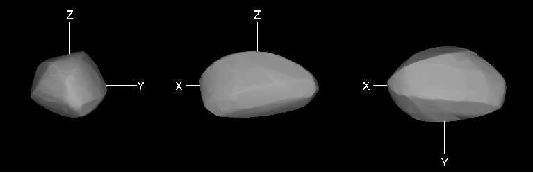
3.7 (6070) Rheinland and (54827) Kurpfalz
This young asteroid pair was studied in detail by Vokrouhlický et al. (2017). Their data are summarized in Table 3 to 5. One of their interesting findings is that the spin vectors of the two asteroids are neither aligned at present nor they were aligned at the time of separation of the two asteroids 16.34 kyr ago, but they were tilted by . We will discuss it in Section 5. The primary (6070) and the secondary (54827) were classified as Sq and Q types, respectively (Polishook et al. 2014). They interpreted the spectral difference as the secondary having a fresher, less space weathered surface.
3.8 (6369) 1983 UC and (510132) 2010 UY57
Backward integrations of their heliocentric orbits suggest that these two asteroids separated about 700 kyr ago (Suppl. Fig. 18). From our observations taken in March-April 2013, we found that the primary (6369) 1983 UC is a binary system. The satellite (bound secondary) has a secondary-to-primary mean diameter ratio of , an orbital period of h, and it is synchronous, i.e., its rotational period is equal to the orbital period (Fig. 19). The fact that we did not observe mutual eclipse events in the system during its 2nd, return apparition in February 2016 indicates that the satellite’s orbit has a significant obliquity, i.e., the orbital pole is not close to the north or south pole of the ecliptic. The primary’s rotational period h is likely. Though we cannot formally rule out a period twice as long, it would be a lightcurve with 8 pairs of maxima and minima per rotation, which is unlikely. We will discuss it, together with other multiple (paired-binary) asteroid systems, in Section 6.

3.9 (7343) Ockeghem and (154634) 2003 XX38
Backward integrations of their heliocentric orbits suggest a lower limit on the age of this pair of 382 kyr (Suppl. Fig. 20). Duddy et al. (2012) found that these two asteroids have very similar spectra belonging to the S class. They also derived the primary’s effective diameter km. With our determined mean absolute magnitude , we obtain the geometric albedo . For the primary (7343), we derived its prograde spin pole (with two mirror solutions in longitude, see Table 5). The best-fit convex shape models for the two pole solutions are shown in Figs. 20 and 21.


3.10 (8306) Shoko and 2011 SR158
Backward integrations of their heliocentric orbits suggest that these two asteroids separated about 400 kyr ago (Suppl. Fig. 21). Pravec et al. (2013) found that the primary (8306) Shoko is a binary, possibly ternary system, from their observations taken during September–December 2013 (see also Pravec et al. 2016). The satellite (bound secondary) has a secondary-to-primary mean diameter ratio of , an orbital period of h, and it is synchronous, i.e., its rotational period is equal to the orbital period. The fact that we did not observe mutual eclipse events in the system during its 2nd, return apparition in January–February 2015 indicates that the satellite’s orbit has a significant obliquity, i.e., the orbital pole is not close to the north or south pole of the ecliptic. The primary’s rotational period h is likely, though we cannot formally rule out a period twice as long with 4 pairs of maxima/minima per rotation. Note that the normalized total angular momentum of the system given in Table 6 was computed without accounting for the possible second satellite (see the references above). Polishook et al. (2014a) found from their spectral observations that it is an Sq type. We will discuss this asteroid system, together with other multiple (paired-binary) asteroid systems, in Section 6.
3.11 (9783) Tensho-kan and (348018) 2003 SF334
This is a secure asteroid pair, showing a good orbital convergence about 600 kyr ago (Suppl. Fig. 24). We found that the primary (9783) Tensho-kan is a binary system. The satellite (bound secondary) has a secondary-to-primary mean diameter ratio of , an orbital period of h and a retrograde orbit with pole near the south ecliptic pole (Scheirich et al., in preparation). The primary’s rotational period is likely, though a period twice that is not entirely ruled out formally. Refining the WISE thermal measurements (Masiero et al. 2011) with our accurately determined mean absolute magnitude of the whole system, , we obtained the effective diameter km and geometric albedo . Correcting it for the satellite presence, we derived the primary’s mean diameter km. We will discuss it, together with other multiple (paired-binary) asteroid systems, in Section 6.
3.12 (10123) Fideöja and (117306) 2004 VF21
Backward orbital integrations of these two asteroids show a modest numbers of clone encounters about 1-2 Myr ago (Fig. 22). This is because the orbits undergo irregular jumps over the 7:2 mean motion resonance with Jupiter. Despite this drawback, we consider this pair to be real, as it is supported also by a good past convergence of the nominal orbits. It is further supported by that the two asteroids have the same colors, as found by Moskovitz (2012), who also classified (10123) as a Ld type, and by our measured and .
We found that the primary (10123) Fideöja is a binary system. The satellite (bound secondary) has a secondary-to-primary mean diameter ratio and an orbital period of h. The primary’s rotational period h is likely, but a period twice as long is also formally possible. In the best data taken in February–March 2013, there is also apparent a second rotational lightcurve with period of h and an amplitude in the combined primary plus secondary lightcurve of 0.04 mag. Whether it belongs to the observed eclipsing secondary or to a third body (second satellite) in the system, remains to be seen from future studies. Refining the WISE thermal measurements (Masiero et al. 2011) with our accurately determined mean absolute magnitude of the whole system, , we obtained the effective diameter km and geometric albedo . Correcting it for the satellite presence, we derived the primary’s mean diameter km. The unbound secondary (117306) 2004 VF21 has a period h (Suppl. Fig. 25). We will discuss the system of Fideöja, together with other multiple (paired-binary) asteroid systems, in Section 6.

3.13 (17198) Gorjup and (229056) 2004 FC126
This is a secure asteroid pair, showing a good orbital convergence about 300 kyr ago (Suppl. Fig. 47). Wolters et al. (2014), following spectral observations by Duddy et al. (2013), found that the primary is Sa while the secondary is Sr type; the secondary has a deeper 1-m absorption band. They suggested that it could be due to a more weathered surface of the primary. Polishook et al. (2014a) reported an Sw type for the primary.
3.14 (21436) Chaoyichi and (334916) 2003 YK39
This is a young asteroid pair, showing an orbital convergence about 30 kyr ago (Fig. 23). We found that the primary (21436) Chaoyichi is a binary system. It has the size ratio and orbital period (Scheirich et al., in preparation). A particularly interesting feature is that it has a non-zero eccentricity of (3- uncertainty). Refining the WISE thermal measurements (Masiero et al. 2011) with our accurately determined mean absolute magnitude of the whole system, , we obtained the effective diameter km and geometric albedo . Correcting it for the satellite presence, we derived the primary’s mean diameter km. We will discuss it, together with other multiple (paired-binary) asteroid systems, in Section 6.

3.15 (25021) Nischaykumar and (453818) 2011 SJ109
Backward integrations of their heliocentric orbits suggest that these two asteroids separated about 900 kyr ago (Suppl. Fig. 59). We found that the primary (25021) Nischaykumar is a binary system. It has the size ratio and orbital period of (Scheirich et al., in preparation). The data suggests that the satellite is synchronous, i.e., its rotational period is equal to the orbital period. The primary’s rotational period h is likely, but we cannot rule out some longer periods for its low amplitude. Refining the WISE thermal measurements (Masiero et al. 2011) with our accurately determined mean absolute magnitude of the whole system, , we obtained the effective diameter km and geometric albedo . Correcting it for the satellite presence, we derived the primary’s mean diameter km. We will discuss it, together with other multiple (paired-binary) asteroid systems, in Section 6.
3.16 (25884) Asai and (48527) 1993 LC1
Backward integrations of their heliocentric orbits suggest that these two asteroids separated about 700 kyr ago (Suppl. Fig. 60). For the primary (25884), using our derived mean absolute magnitude , we refined the WISE data by Masiero et al. (2011) and obtained km and . Polishook et al. (2014a) found it to be an X type in the near-IR Bus-DeMeo taxonomy system. Considering its high albedo and position in the Hungaria asteroid family, it probably belongs to the E class in the Tholen taxonomy. We also derived its retrograde spin pole (see Table 5). The best-fit convex shape model is shown in Fig. 24.

3.17 (26416) 1999 XM84 and (214954) 2007 WO58
This is a secure asteroid pair, showing a good orbital convergence about 270 kyr ago (Suppl. Fig. 61). Polishook (2014b) suggested from observations taken from Wise in 2011 that the primary (26416) 1999 XM84 is a binary system, and we confirmed it with observations from La Silla in 2015 (Pravec et al. 2015). The satellite (bound secondary) has a secondary-to-primary mean diameter ratio , an orbital period of h and a retrograde orbit with pole within 10∘ of the south ecliptic pole (Scheirich et al., in preparation). The satellite is synchronous, i.e., its rotational period is equal to the orbital period. The primary’s rotational period h is likely, though a period twice that is not formally ruled out. The rotational period of the unbound secondary (214954), h is likely (Suppl. Fig. 62), though a period twice that with four pairs of lightcurve maxima and minima per rotation is also possible. We will discuss it, together with other multiple (paired-binary) asteroid systems, in Section 6.
3.18 (26420) 1999 XL103 and 2012 TS209
This is a secure asteroid pair, showing an orbital convergence about 250 kyr ago (Suppl. Fig. 63). We found that the primary (26420) 1999 XL103 is a binary system. The satellite (bound secondary) has a secondary-to-primary mean diameter ratio and an orbital period of h or h (Suppl. Figs. 64 and 65). The primary’s rotational period has not been uniquely determined, there are a few possible solutions from 2.2 to 4.2 h. From our Sloan color measurements, we derived that it is a V type. We will discuss it, together with other multiple (paired-binary) asteroid systems, in Section 6.
3.19 (42946) 1999 TU95 and (165548) 2001 DO37
Backward integrations of their heliocentric orbits suggest that these two asteroids separated about 700 kyr ago (Suppl. Fig. 77). From our measured Sloan colors, we found that both asteroids are S types. Polishook et al. (2014a) reported that the primary is an Sr or Sw type. Using our derived weighted mean absolute magnitude , we refined the WISE data by Masiero et al. (2011) and obtained km and ; it is an albedo typical for S types.
3.20 (43008) 1999 UD31 and (441549) 2008 TM68
Backward integrations of their heliocentric orbits suggest that these two asteroids separated about 270 kyr ago (Fig. 25). From our observations taken during December 2014-January 2015, we found that the primary (43008) 1999 UD31 is a binary system. The satellite (bound secondary) has a secondary-to-primary mean diameter ratio and an orbital period of h (Fig. 26). The fact that we did not observe mutual eclipse events in the system during its 2nd and 3rd, return apparitions in April 2016 and September–October 2017 (Figs. 27 and 28) indicates that the satellite’s orbit has a significant obliquity, i.e., the orbital pole is not close to the north or south pole of the ecliptic. The satellite is synchronous, i.e., its rotational period is equal to the orbital period. The primary’s rotational period h is likely, but we cannot rule a period twice that with six pairs of lightcurve maxima/minima per rotation. The unbound secondary (441549) has a likely period h, but other nearby periods are not ruled out (Suppl. Fig. 81). We will discuss the system of (43008), together with other multiple (paired-binary) asteroid systems, in Section 6.


3.21 (44620) 1999 RS43 and (295745) 2008 UH98
Backward integrations of their heliocentric orbits suggest that these two asteroids separated about 700 kyr ago (Suppl. Fig. 82). We found that the primary (44620) 1999 RS43 is a binary system. The satellite (bound secondary) has the secondary-to-primary mean diameter ratio , an orbital period of h and a prograde orbit with pole within 7∘ of the north ecliptic pole (Scheirich et al., in preparation). The satellite is synchronous, i.e., its rotational period is equal to the orbital period. The primary’s rotational period h is likely. Though a period twice that is not formally ruled out, it would be a complex lightcurve with numerous maxima/minima per rotation, which is unlikely. From our measured Sloan colors, we derived that the primary is an S type. We will discuss it, together with other multiple (paired-binary) asteroid systems, in Section 6.
3.22 (46829) McMahon and 2014 VR4
This asteroid pair is probably real; we calculated the probability that it is a random orbital coincidence of two independent asteroids . For backward integrations of their heliocentric orbits, we used 3000 orbital clones for the primary and 10000 clones for the secondary. We chose that because the orbit of 2014 VR4 is not very accurately determined yet so we sampled its large uncertainty hyperellipsoid with ten times more clones than for other asteroid pairs. The orbital clones show a convergence about 800 kyr ago (Fig. 29). We found that the primary (46829) McMahon is a binary system. The satellite (bound secondary) has a secondary-to-primary mean diameter ratio of and an orbital period of h (Figs. 30 and 31). The primary’s rotational period h or twice that. We will discuss it, together with other multiple (paired-binary) asteroid systems, in Section 6.


3.23 (49791) 1999 XF31 and (436459) 2011 CL97
Backward orbital integrations of these two asteroids showed a relatively low number of clone encounters (Fig. 32). This is probably because of a strong Yarkovsky effect for the small secondary, for which our coverage with 1000 orbital clones is not very dense. Contributing to it may be also a strong chaoticity of their orbits (probably due to the 15:8 mean motion resonance with Mars). We calculated that the probability that this pair is a random coincidence of two independent asteroids in the space of mean orbital elements is 3%. We consider this pair to be probably real, but it will have to be confirmed with future studies. For the primary (49791), V type is a likely classification from the SDSS measurements, though our measured differs from the mean for V types (Pravec et al. 2012b) by more than ; a confirmation of the taxonomic classification with further observations will be needed. The period of (49791), h is likely, but a value twice that with 4 pairs of lightcurve maxima/minima per rotation is not entirely ruled out (Suppl. Fig. 86). With the , this primary rotation is too slow for formation of this asteroid pair by rotational fission. We will discuss this anomalous case, together with other two similar ones, in Section 6.

3.24 (52852) 1998 RB75 and (250322) 2003 SC7
Backward integrations of their heliocentric orbits suggest that these two asteroids separated about 500 kyr ago (Suppl. Fig. 93). Polishook et al. (2014a) found that the primary (52852) is a V type. Its rotational period is estimated h, but half-integer multiples of this value are also possible. In our observations taken in September-October 2015, there appeared several brightness attenuations about 0.06 mag deep that might be mutual events due to a satellite of the primary, but we did not obtain a satisfactory solution for period of the suspect events. A confirmation with future high-quality observations is needed.
3.25 (53537) 2000 AZ239 and (503955) 2004 ED107
This is a secure pair. Backward integrations of their heliocentric orbits suggest that these two asteroids separated about 500 kyr ago (Fig. 33). However, the pair has an anomalously low angular momentum content. The primary’s spin period was uniquely determined h, there is no ambiguity or significant uncertainty in it (Fig. 34). In particular, all shorter periods are ruled out. With the pair’s , it is a too slow primary rotation to be explained by the theory of pair formation by rotational fission. We will discuss this and other two similar anomalous cases in Section 6.


3.26 (54041) 2000 GQ113 and (220143) 2002 TO134
This is a secure pair. The two asteroids are close one to each other ( m/s, ) and they show a good orbital convergence with estimated age about 200 kyr (Suppl. Fig. 96). The period of (54041) is ambiguous, it is either h or twice that. The period of (220143) h is likely. Though a period twice as long cannot be formally ruled out, it would be a complex lightcurve with numerous maxima and minima, which seems implausible. See Suppl. Figs. 97 to 102. With the mean value (see Electronic Supplementary Information), we refined the WISE effective diameter and geometric albedo (Masiero et al. 2011): km and . We measured the color indices and ; the former value is consistent with the V type found for the primary by Polishook et al. (2014a).88 8 From SDSS measurements, (54041) is suggested to be an S type. These two color indices differ by , i.e., the difference is significant at 2- level. It will be good to do a spectral study of this asteroid pair in the future.
3.27 (56232) 1999 JM31 and (115978) 2003 WQ56
Backward integrations of their heliocentric orbits suggest that these two asteroids separated about 130 kyr ago (Suppl. Fig. 109). For the primary (56232), we derived its retrograde spin vector (see Table 5). The best-fit convex shape model is shown in Fig. 35.

3.28 (57202) 2001 QJ53 and (276353) 2002 UY20
This is a secure pair. Backward integrations of their heliocentric orbits suggest that these two asteroids separated about 130 kyr ago (Suppl. Fig. 116). The rotational period of the primary (57202) is likely h; periods twice or thrice as long are not entirely ruled out, but appear implausible (Suppl. Figs. 117 and 118). From the SDSS measurements, it is likely an S type, though an L type cannot be entirely ruled out. In our observations taken in January 2017, there occurred two brightness attenuations 0.08–0.11 mag deep that could be mutual events due to a satellite of the primary. This probable paired binary needs to be confirmed with future observations.
3.29 (60677) 2000 GO18 and (142131) 2002 RV11
This is a secure pair. Backward integrations of their heliocentric orbits suggest that these two asteroids separated about 140 kyr ago (Fig. 36). The period of (60677), h is likely, but a value twice that with 4 pairs of lightcurve maxima/minima per rotation is not entirely ruled out (Figs. 37 and 38). The period of (142131), h is likely; a value twice that does not appear plausible (Fig. 39). From the SDSS colors, we derived that the secondary belongs to S, A or L class. However, a particularly interesting feature of this pair is that it has a low , i.e., an anomalously high mass ratio . This is not predicted for an asteroid pair with fast rotating primary by the theory of rotational fission. We will discuss this anomalous case, together with other three similar ones, in Section 6.


3.30 (60744) 2000 GB93 and (218099) 2002 MH3
Backward integrations of their heliocentric orbits suggest that these two asteroids separated about 350 kyr ago (Suppl. Fig. 121). We measured the color indices and . From the SDSS measurements, we classify the primary as an S type. We also derived its retrograde spin vector (see Table 5). The best-fit convex shape model is shown in Fig. 40.

3.31 (69142) 2003 FL115 and (127502) 2002 TP59
Despite the somewhat increased distance between these two asteroids ( m/s) and its relatively high estimated about 1 Myr (Suppl. Fig. 134), it appears to be a real pair. For the primary (69142), we derived its prograde spin vector (see Table 5). The best-fit convex shape model is shown in Fig. 41.

3.32 (76148) 2000 EP17 and (56048) 1998 XV39
This is a secure pair. Backward integrations of their heliocentric orbits suggest that these two asteroids separated about 1 Myr ago (Fig. 42). For (76148), we found a long period with the formal best fit h, but it is not an unique solution and its exact period has to be derived from future observations (Suppl. Fig. 144). For (56048), we derived its prograde spin pole (with two mirror solutions in longitude, see Table 5). The best-fit convex shape models for the two pole solutions are shown in Figs. 43 and 44. We also measured their color indices and . What is, however, particularly interesting is that these two asteroids have about the same absolute magnitudes; , i.e., the mass ratio . This is not predicted for an asteroid pair formed by rotational fission. We will discuss this anomalous case, together with other three similar ones, in Section 6.


3.33 (80218) 1999 VO123 and (213471) 2002 ES90
This is a secure asteroid pair, showing an orbital convergence about 140 kyr ago (Fig. 45). We found that the primary (80218) 1999 VO123 is a binary system. The satellite (bound secondary) has a secondary-to-primary mean diameter ratio , an orbital period of h, and it is synchronous, i.e., its rotational period is equal to the orbital period (see Pravec et al. 2016). The primary’s rotational period h is likely; a period twice as long with 4 pairs of lightcurve maxima and minima per rotation is formally not ruled out, but it appears unlikely. The period of the unbound secondary (213471), h is well established (Fig. 46). We measured their color indices and ; an excellent agreement. However, it is even more interesting, as this asteroid pair has an anomalously low . After a correction of for the satellite presence, it is , i.e., it is a high mass ratio . We will discuss this very interesting asteroid system in Section 6.


3.34 (101703) 1999 CA150 and (142694) 2002 TW243
Despite the large distance between these two asteroids in mean elements ( m/s), caused by interaction with the secular resonance, this appears to be a real pair. Backward integrations of their heliocentric orbits suggest its age about 700 kyr (Fig. 47). The primary (101703) was found to be an Sw or Q type (Polishook et al. 2014). Its rotation period h is well established. However, in the data of 2009-09-20.2, there appeared a brightness attenuation that could be a mutual event due to a satellite of the primary (see Suppl. Fig. 38 in Pravec et al. 2010). Moreover, in our accurately calibrated data taken in October 2013, there appears to be a second lightcurve component with a period on an order of 50–60 h that might be a rotational lightcurve of the suspected satellite (Fig. 48). The suggested binary nature of (101703) will have to be confirmed with future observations.


3.35 (122173) 2000 KC28 and (259585) 2003 UG220
This is a secure pair. Backward integrations of their heliocentric orbits suggest that these two asteroids separated about 250 kyr ago (Fig. 49). The period of (122173), h is likely, but half-integer multiples of it are not ruled out (Fig. 50). The period of (259585) was not accurately established, a value of h appears possible (Fig. 51), but some longer periods are possible as well. We measured their color indices and ; an excellent agreement. However, a particularly interesting feature of this pair is that it has a low , i.e., an anomalously high mass ratio . This is not predicted for an asteroid pair with fast rotating primary by the theory of rotational fission. We will discuss this anomalous case, together with other three similar ones, in Section 6.


4 Albedos, colors and taxonomic classes
We obtained geometric albedos , refined from the WISE data (Masiero et al. 2011) with our accurate absolute magnitudes using the method described in Pravec et al. (2012b), for 31 asteroid pair primaries. The data are given in the 3rd column of Table 4 and they are plotted in Fig. 52. 27 of the 31 pairs have medium albedos between 0.14 and 0.32, while 2 and 2 are low- and high-albedo asteroids ( about 0.04 and about 0.49), respectively. The scarcity of low-albedo asteroid pairs in our sample is suspected to be due to a bias against their detection, as the pair secondaries are mostly small (on an order of 1 km) and the known population of main belt asteroids at these diameters is heavily biased towards higher albedo objects due to the magnitude-limited sky surveys in the visual spectral range. For 74 asteroid pairs, we obtained color indices for one or both components. The data are given in the 6th and 7th columns of Table 4 and plotted in Fig. 53. Nearly 3/4 (53 of the 74) of the asteroid pairs have in the range 0.44–0.52, which is a range predominated by the S complex and where also Q, V and L type asteroids are. The tail towards lower values, down to 0.34, is likely a mixture of blue-end members of the SQ complex, X types, and neutral reflectance (solar-like color)99 9 The solar is . primitive (C and C-like) types. From Fig. 54 where we plot the vs data for 26 asteroid pairs where we got both, it is apparent that most (or all, for our specific sample) asteroid pairs with the values from 0.42 to 0.51 have medium albedos, consistent with them being (mostly) S/Q/L types (see below). Two of the three points with neutral to slightly red values from 0.36 to 0.40 are low-albedo objects and one has a medium albedo; the former are probably primitive (C/C-like) types and the latter, (11286) is an X/M type. Though unique taxonomic classifications cannot be given from the single-color data, the observed distribution of the albedos and colors is consistent with what we see in the general population of the main asteroid belt if we consider the observational bias against small low-albedo asteroids.
The taxonomic classifications that we obtained from spectral or color measurements for one or both components of 42 asteroid pairs (given in the 4th and 5th columns of Table 4) generally confirm the picture suggested from the albedos and color indices above. 28 of the 42 are S, Q or L types, 8 are X (mostly E) types, 4 or 5 (one classification is uncertain) are V types, and 1 is a Ch type. In 9 cases, we obtained taxonomic classifications for both components. One of the 9 is an X type and 8 belong to the SQ complex. It is significant that in all the 9 cases, both components of a given pair belong to the same taxonomic complex, with no or only moderate difference between them. In three cases (see Table 4), we see that the secondary is apparently less space weathered, having stronger absorption features (Q, Sq, Sr) than the primary (Sq, S, Sa). It suggests that in at least some asteroid pairs, the secondary has a fresher surface than the primary.


5 Spin and orbit poles
We determined spin or orbit pole positions for 19 asteroids or asteroid binaries in 17 asteroid pairs. The data are presented in Table 5 and the referenced subsections in Section 3. We analyse them in below.
Of the 17 asteroid pairs with determined poles (for at least one pair member), 7 are prograde and 10 retrograde. The slight preference for retrograde poles is not statistically significant.
There is an apparent concentration of the determined asteroid pair poles to the north and south poles of the ecliptic. However, its reality needs to be confirmed with simulations of selection effects affecting the sample; there is present an observational/modeling bias against asteroids with high obliquities. Note that for asteroids with low obliquities, their poles can be uniquely (in latitude at least) derived with less amount of data typically than for asteroids with obliquities close to 90∘ (for that the latter have lower mean observed lightcurve amplitudes on average, due to the projection effect). The selection effect is even stronger for asteroid binaries for which we need to observe typically 3 apparitions with mutual events in order to derive an unique orbital pole. For binaries with high obliquities that are in eclipse/occultation geometry and therefore show mutual events in only some apparitions, it means that we need to observe them in many more apparitions than for binaries with low obliquities which show mutual events most or all the time. Such multi-apparition data are not available for the binary systems in our asteroid pairs sample yet. Hence all the four binaries in Table 5 have close to or . For three other paired binaries that we re-observed in their 2nd or 3rd apparition (after the discovery of their binary nature in the 1st apparition), namely (6369), (8306) and (43008) (see their subsections), there were not present mutual events in the return apparitions, indicating that their obliquities are not low. Note that for general main-belt asteroid binaries, we simulated the observational selection effects and found a real strong concentration of their poles towards the ecliptic poles (Pravec et al. 2012a), but we will need to do the de-biasing for paired binaries when sufficient data are available in future.
For two pairs, 2110–44612 and 6070–54827, we determined poles of both pair members. The important finding is that in each of the two pairs, both members have the same sense of rotation (retrograde in both cases). The pair 6070–54827 was studied in detail by Vokrouhlický et al. (2017) who found that the original spin vectors of the two asteroids were not co-linear but tilted by at the time of their separation. In the case of 2110-44612, we found that though the 3- uncertainty areas of their pole positions overlap (see Suppl. Figs. 1 and 2), their nominal pole positions (for both mirror solutions) differing by about 90∘ in longitude call for a more detailed look into the long-term evolution of asteroid spin poles. We present it in following.
From our observations, we determine an asteroid spin vector at the present epoch. In the optimum situation, we have information on the spin axes of both components of an asteroid pair. However, we want to know what were their spin axes right after formation of the pair, as such data can be confronted with predictions from the theories of asteroid pair formation. A question arises to what degree the current spin configuration preserves the original configuration. Here we give a brief look to this problem, having in mind the sample of paired asteroids for which we derived their spin poles (Table 5). These bodies are large enough, and their estimated ages short enough, so that we may neglect non-gravitational effects, such as YORP, in the first approximation. However, the spin axis orientation is affected by gravitational torques, primarily from the Sun, which may tilt the original spin vectors on a timescale comparable to or shorter than the pair ages. Therefore, we must consider their effect for the pairs.
Breiter et al. (2005) presented an efficient numerical implementation of the secular spin dynamics due to the solar torques. Because this problem is tightly coupled with orbital dynamics, in particular changes in orientation of the orbital plane in the inertial space, we also need to propagate the heliocentric orbit over the same interval of time for which we seek the spin evolution. To infer this information, we embedded the secular model of Breiter et al. (2005) into the symplectic orbit-evolution package swift (e.g., Levison and Duncan 1994). The initial data for the orbit integration are taken from the AstDyS web site. We first integrate the nominal orbit of the asteroid backward in time to reach the inferred epoch of the pair formation. At that moment, we set up initial data for the spin integration and propagate both the orbit and spin forward in time to the current date. The spin integration requires the value of the precession constant to be known. Apart from the orbital data, depends also on the spin rate and the dynamical flattening of the asteroid. The spin rate is known well from our observations, but the flattening is determined only approximately with our convex shape model. In particular, where are the principal values of the inertia tensor. We assume a homogeneous density distribution in the asteroid when estimating these values. However, an analysis of shape variants that also satisfy the photometric data implies that is known with only % accuracy typically for asteroid convex shape models. The situation is even more complicated when the asteroid has a satellite. The effective value then depends also on the orbital and physical parameters of the satellite (see Sec. 5.1.1 of Pravec et al. 2012a). The necessary data are taken from our observations (Table 5) that allow to estimate the required quantities. As above, the value of is known with poor accuracy, contributing by the largest value to the uncertainty in the precession constant . In order to sample possible outcomes of the spin evolution, we propagate different variants for which the precession constant has been fractionally changed by % from the nominal value.
The simplest situation occurs for very young pairs, for which the today’s pole orientation may still be relatively close to its original value. For instance, in the case of the 6070–54827 pair, the relative configuration of the primary and secondary asteroid poles did not change much. This is because (6070) has a nearly stationary spin axis directed at the south ecliptic pole, while the spin pole of (54827) performed only a displacement along a constant ecliptic latitude. When the age is higher, and the rotation sense is retrograde, the regular precession may smear the pole location to all possible ecliptic longitudes. As an example, we note that it is important to consider this effect when interpreting our result for the 2110–44612 asteroid pair. In this case, our solution gives the nominal poles of both components having about the same ecliptic latitude and the ecliptic longitudes about different. This result is, however, entirely compatible with an initially co-linear configuration of the spins of the primary and the secondary. Figure 55 shows an example of the evolution of the pole orientation for the primary (2110) Moore-Sitterly, assuming an age of Myr and the nominal value . Note that the obliquity performs only small oscillations (keeping the ecliptic latitude nearly constant), while the ecliptic longitude of the asteroid spin axis undergoes regular precession around the south ecliptic pole with a period of about kyr. The evolutionary track of the secondary’s spin pole is similar with only a different value of the precession period (because of its different value of the rotation period and dynamical flattening). So their poles diverge in the ecliptic longitude to acquire any longitudinal difference at a future time. That said, we obviously cannot prove initial co-linearity of the rotation poles in the 2110–44612 pair, but the data are consistent with that. In any case, the poles are never more than apart during their evolution. This is because of their proximity to the south ecliptic pole and the low inclination of their heliocentric orbits.

However, things may get much wilder for prograde rotating asteroids residing on high-inclination heliocentric orbits. This is because precession rate for prograde-rotating asteroids may occur to be in resonance with precession rate of the orbital plane (e.g., Colombo 1966, Henrard and Murigande 1987). Specific examples of secular spin axis evolution for asteroids in the inner main belt, where most of our studied pairs reside, can be found in Vokrouhlický et al. (2006) or Vraštil and Vokrouhlický (2015).
The most significant perturbations occur for pairs among Hungaria asteroids, whose orbital inclinations are high. To demonstrate the effects, we consider the case of (4765) Wasserburg, the primary component of the 4765–350715 pair (Section 3.4). We found that (4765) has a peculiarly large obliquity of , which seemed to be at odds with the expected low obliquities of paired asteroids after YORP-induced fission, close to the YORP asymptotic obliquity values. For sake of definiteness, we assume an age of kyr for the 4765–350715 pair, consistent with its estimated age, and consider the value from the (4765)’s nominal convex shape model. Most importantly, we assume that the initial obliquity at the formation of the pair was only, very different from the today’s value. With these data, we propagated the nominal model plus 19 clone variants by taking slightly different values and initial longitudes of the spin axis. Evolution of the obliquity for all these cases is shown in Fig. 56. There are two main features to be noted: (i) the obliquities oscillate up to , and (ii) the different cases quickly diverge, achieving at the current epoch any value between and obliquity. This is because the nominal value of the precession constant arcsec/yr is close to the principal frequencies arcsec/yr and arcsec/yr with which the orbital plane precesses in space. The proper inclination is high, , and it implies a stationary point (Cassini state 2) of the spin-orbit resonance with the -frequency at about . A similar stationary point for the -frequency is at about , enclosed with a resonance zone spanning from to obliquity. Interaction of the two phenomena forms a large chaotic zone for the obliquity evolution extending to nearly . As a result, we find that the current position of the spin pole of (4765) cannot be used to determine its initial spin vector orientation. We may also imagine that the pole position of the secondary (350715) could follow one of the tracks shown in Fig. 56 that end at a near-zero obliquity. Therefore, a potential large angular distance of current poles of the members of this pair would still be perfectly compatible with them being co-linear right after the pair formation. The same analysis applies also to the asteroid (69142) 2003 FL115, the primary component of the 69142–127502 pair.

The huge obliquity variation discussed above for (4765) is closely related to the prograde sense of its rotation. Retrograde rotators among Hungarias show much smaller effects, principally produced by the large orbital inclination. We tested this conclusion in the case of asteroid (25884) Asai, for which we determined the current obliquity of (Section 3.16 and Table 5). Adopting an age of kyr, compatible with the estimated age of the pair 25884–48527, we repeated our numerical experiment by propagating 10 possible variants of pole evolution for (25884), starting with an initial obliquity of . The results are shown in Fig. 57. The obliquity oscillations are now limited to a relatively narrow range between and . Note that their amplitudes are even smaller than the proper orbital inclination of and the oscillations have now a short period of kyr. This is because for retrograde rotators the regular spin precession is opposite to the orbital plane precession and may not constitute a resonant configuration. As a result, the today’s obliquity should preserve the initial value to within about (which is smaller than the 3- uncertainty of the pole solution). Obviously, the ecliptic longitudes of spin poles of members of a pair older than a half million years can be very different.
Using the tools described above, we analysed all the other paired asteroids with determined spin poles reported in Table 5. We found no significant secular effects that would surpass the solution uncertainty with possibly an exception of (56048) 1998 XV39. This is the secondary of the anomalous high-mass ratio pair 76148–56048 (see Sections 3.32 and 6.1). We find that its current to obliquity may be acquired from an initially low obliquity through chaotic evolution due to overlap of the and secular spin-orbit resonances.
Our analyses above can be briefly summed up as follows: The present-epoch pole orientation of a paired asteroid typically does not represent its original state. Effects of the spin evolution over the age of an asteroid pair need to be taken into account. In the simplest case, the spin dynamics represents only the regular precession in ecliptic longitude. For low- and mid-latitude pole positions, this effect may cause a large angular separation of the primary and secondary poles at the current epoch. In more complicated cases, generally those of prograde-rotating asteroids residing on high-inclination heliocentric orbits, the pole evolution may be chaotic, even to a degree preventing a deterministic connection of the present pole position with its initial value. We conclude that each asteroid pole solution needs to be analysed individually. Overall, of the 17 pairs in this sample, we found that 13 show low-amplitude oscillations of their obliquities (smaller than their uncertainties), other 2 —(25884) and (56048)— show moderate oscillations (comparable to the uncertainties of their obliquities), and the last 2 —the prograde-rotating Hungarias (4765) and (69142)— show high-amplitude oscillations.

6 Primary period vs mass ratio distribution, and bound secondaries (paired binaries)
In Fig. 58, we plot the primary period vs pair mass ratio data for the 93 studied asteroid pairs. The filled circles are data with securely determined primary periods (with the period determination quality code ), while the diamonds are data where the primary periods are uncertain by a factor of 1.5 typically, up to 2, usually due to uncertainty of a number of observed lightcurve maxima/minima per rotation (). The black dashed curve is the nominal relation between the primary period and mass ratio computed from the theory of formation of asteroid pairs by rotational fission, and the blue, red and green solid curves are theoretical limits (lower or upper) on the primary rotation frequency as derived in Pravec et al. (2010, 2018). Specifically, the black dashed curve is for the normalized total angular momentum of the system , the primary’s equatorial elongation , , and the initial relative semi-major axis . This set of parameters can be considered as the best representation of pair parameters. In particular, the total angular momentum content of 1.0 is about the mean of the distribution of values in small asteroid binaries (Pravec and Harris 2007), and the axial ratio of 1.4 is about a mean of equatorial elongations of pair primaries suggested by their observed amplitudes. The red and blue curves represent upper and lower limit cases. The upper curves are for the system’s normalized total angular mometum , primary’s axial ratio , and initial orbit’s normalized semi-major axis and 4. The lower curves are for and and 4. The choice of for the upper limit cases is because the asteroid pair primaries closest to the upper limit curve have low amplitudes –0.2 mag. Similarly, the choice of for the lower limit cases is because the highest amplitudes of the points close to the lower limit curve are –0.5 mag, suggesting the equatorial elongations –1.5. For completness, the green curve gives the theoretical hard upper limit on the final primary spin rate (i.e., lower limit on the period) as derived in Pravec et al. (2018). As discussed in that paper, the theoretical hard limit was derived involving certain idealizations that are probably not fulfilled in real asteroids. In particular, it assumes spherical component shapes while real asteroids are non-spherical. Thus, real asteroid pairs formed by spin-up fission may stay well below the theoretical hard limit. Indeed, we see in the plot that the observed asteroid pairs do not extend to the green curve at about 0.6, but they are well to the right of the curve (except for the four anomalous high-mass ratio pairs —the four leftmost points in Fig. 58—, which we will discuss below).

6.1 Outliers to the – relation
Of the 93 asteroid pairs in our sample, 86 follow the – relation derived from the theory of asteroid pair formation by rotational fission. Of the 7 outliers, 3 have too slow primary rotations (too low total angular momentum content; they lie below the blue curves in Fig. 58) and 4 have too high mass ratios (they are to the left of the upper limit curves in the plot).
The 3 low-angular momentum pairs are 49791–436459 (Sect. 3.23), 53537–503955 (Sect. 3.25) and 69298–2012FF11. In the last case, it may be due to a possible error in its or value; we cannot entirely rule out that the period of (69298) is in error by a factor of 2 if it has a monomodal lightcurve, or the absolute magnitude of the secondary 2012 FF11 taken from MPC may be in error. Thus, the anomalously low angular momentum content of this pair has to be confirmed with accurate measurements of the two uncertain parameters in the future. The other two asteroid pairs appear to be real outliers; it is unlikely that their and values could have big errors. However, in the case of 49791–436459, we have to consider the possibility that it may not be a real pair, but that it may be a random orbital coincidence of two unrelated asteroids, see Sect. 3.23. The case of 53537–503955 is, however, a securely established pair (see Sect. 3.25) and it is a true outlier — the lowest point at in the – plot. We do not have a physical theory for how it could be formed with such slowly rotating primary and very small secondary. Just, we consider a possibility that it might not be actually an asteroid pair, but an asteroid cluster, similar to the clusters studied in Pravec et al. (2018), with its more secondaries with sizes similar to (503955) waiting to be discovered in the future. With a few more secondaries with sizes of 0.5–1 km, its mass ratio would rise to that would be in agreement with the theory of asteroid cluster formation. We note that the known main belt asteroid population is highly incomplete at asteroid diameters km —we estimate a diameter of km for (503955)— so there may exist yet-to-be-discovered secondaries of the putative cluster of (53537). We conclude that all the three anomalous pairs with apparently too low angular momentum content may be just due to our uncertain or incomplete knowledge and they do not represent a real challenge to the theory of asteroid pair formation by rotational fission.
The 4 anomalous high-mass ratio pairs are 60677–142131 (Sect. 3.29), 76148–56048 (Sect. 3.32), 80218–213471 (Sect. 3.33) and 122173–259585 (Sect. 3.35). All the four pairs were securely identified, there is no doubt about their reality. Three of the four form a compact group in the upper left of Fig. 58. They share a number of common properties. All the 6 members (3 primaries and 3 secondaries) of the three pairs rotate fast, with periods from 2.7 to 4.7 h and they have low lightcurve amplitudes mag that suggest that they have nearly spheroidal shapes with the equatorial axis ratios . They are small; we estimate their diameters 1–2 km. The three pairs are relatively young, their likely ages are between 100 and 300 kyr. They were not taxonomically classified yet; the color indices and positions in the inner main belt suggest that the pairs 60677–142131 and 122173–259585 could belong to the SQ complex, while 80218–213471 might be more likely an X type. The fourth pair, 76148–56048 is somewhat separated in certain properties from the three of the compact group: Its members rotate slower ( and 7.0 h) and it is older (estimated age kyr), but, like the other three pairs, it is small asteroids ( km; see Electronic Supplementary Information) with low lightcurve amplitudes, and it likely belongs to the S complex (based on its color indices, geometric albedo, and position in the inner main belt). And, to make it even more interesting, the primary of the pair 80218–213471 has a bound, orbiting synchronous secondary, see Sect. 3.33 and Table 6.
The 4 outlier asteroid pairs present a challenge for the fission theory that seems to explain the other population of asteroid pairs. Definitive results on how they formed will require additional information and observations of these systems. In their absence, we can analyze the extreme energetics of fissioning and reshaping systems to understand what the general theory can say about the limits. First, we note that the fission theory applied to the other asteroid pairs assumes that the bodies themselves do not undergo reshaping following fission. At most, we may assume that they fission again, but remain rigid. If we relax this assumption and allow for the fissioned components to reshape themselves into more spherical shapes, then additional energy can be liberated from the system and can allow asteroid pairs with mass ratios approaching unity.
We note that the 4 outlier asteroid pair systems have relatively unelongated shapes that may be consistent with this scenario, and thus we attempt to apply this generalized fission theory under the assumption that the bodies reshaped themselves after fission. The main elements of the calculations we carry out are given in Scheeres (2004). Here we assume that the parent body is an ellipsoid with a given self-potential energy and kinetic energy from rotation. If it rotates fast enough, it can fission and split into two bodies with masses that sum to the total mass of the initial body. If we assume that these two bodies take on nearly spherical shapes, this releases additional energy which the system can use to disrupt.
This process can be simply represented if we only allow the different shapes to take on ellipsoidal shapes, as we can evaluate the self potentials in closed form. The general fission process for a single body yields the balance equation
| (3) |
where is the mass of the parent body, is the mass fraction of the two bodies, is the moment of inertia of the th body (assumed to be its maximum moment of inertia), is its spin rate, is the self-potential of the body, and and are the relative velocity and the mutual potential between the fissioned bodies. Here is the parent body which splits into bodies 1 and 2. The free energy of the fissioned system is
| (4) |
and is normally taken as a constant. We note that the free energy must be positive for the two bodies to be able to escape from each other (Scheeres, 2002), and is the fundamental property that the fission theory of asteroid pairs is founded on. If the two bodies escape from each other, then and . The limiting case is for and it provides a constraint on the final spin rates of the separated bodies,
| (5) |
For the current analysis we note that if bodies 1 and 2 deform into a lower energy configuration then this can in fact increase the overall free energy available and potentially allow for larger mass ratios to escape. The current analysis explores the energetic limits of these systems without necessarily proposing this as a true physical solution for their existence.
To model this we treat the parent body as a triaxial ellipsoid with semi-major axes , which allows us to compute the self-potential of the body and the spin rate at which the body should undergo disaggregation (see Scheeres, 2004, for these details). Then, for a given mass fraction split between the bodies, to maximize the free energy we must take , which is the self-potential of a sphere of mass and radius and minimizes the self-potential over all possible shapes. Similarly, to maximize the resulting spin rates we take the moments of inertia towards that of a spherical body , which minimizes the maximum moment of inertia over all possible constant density ellipsoidal shapes. Finally, for the constant density constraint and mass conservation we note that and , where is the geometric mean radius of the original body.
Then, for an assumed initial ellipsoidal shape we can calculate whether the bodies can escape and what their expected spin rates are if they do escape. Figure 59 shows this calculation for , meaning that the bodies split into equal masses. This figure shows the possible final rotation rate (in terms of the surface disruption spin rate) as a function of the axis ratios of the initial ellipsoid. It also assumes that the two bodies spin at the same rate after escape. Also plotted are the size ratios of the Maclaurin and Jacobi ellipsoids. We note that Maclaurin and Jacobi ellipsoids near the bifurcation point between them can have enough energy to allow their fissioned components to escape if those bodies are allowed to reshape into a spherical shape, however the spin rate of those bodies would be expected to be low. If a body is significantly distended, however, then the bodies can escape with a larger spin rate. Thus, from this simple analysis we see that it may be energetically possible for our outlier asteroid pairs to be formed from a fission event — albeit a very specific set of physical transformations would be required.

Given this result, we can compute similar energy curves for each of our candidate outlier asteroid pairs. Here we assume the specific mass fraction for each pair, assume their respective spin rates (normalized by a spin period of 2 hours which we take as a proxy for these being likely mostly S type asteroids), and then compute the line of progenitor ellipsoid shapes that would supply sufficient energy for the current configuration (assuming the individual bodies are spheres). Figure 60 presents these results. For the different pairs Table 7 presents the different mass fractions and normalized spin rates.

We see that for the three more rapidly spinning pairs this would require a relatively flattened parent asteroid, requiring an oblate body to have from 0.4 to 0.6 across these three. For the slowly rotating body, we see that a Maclaurin Spheroid could lead to this situation. However, we note that the members of the 4 outlier asteroid pairs are actually not spherical as assumed in the calculations above, but they have certain equatorial elongations producing the non-zero observed lightcurve amplitudes (and their polar flattenings are largely unconstrained). Thus, if this scenario with pair component reshaping after fission is true, then the original parent body must be even more flattened than suggested by the above calculation. Finally, we admit that we do not know a mechanism that could reshape the fissioned components into relatively unelongated bodies as we observe in the 4 outlier asteroid pairs. We conclude that a formation process for the 4 outlier asteroid pairs remains unknown.
6.2 Asteroid pairs with binary primaries
An extremely interesting finding is that many of the fastest rotating primaries of asteroid pairs have also bound, orbiting secondaries. We found 13 such cases, see Table 6. In fact, of the 34 asteroid pairs with h in our sample, the 13 ones with binary primaries represent a fraction of 38%. And considering that the binary asteroid detection probability of the photometric method is substantially less than 100% (see Pravec et al. 2012a), it is likely that a true fraction of binary systems among the fastest rotating primaries of asteroid pairs is actually at least 50%.1010 10 A few more possible binaries among asteroid pair primaries are marked with “?” in the column “Sat.1” in Table 3. They await confirmation with further observations. It may be comparable to the binary fraction among the fastest rotating near-Earth asteroids larger than 0.3 km that is % (Pravec et al. 2006). The 13 asteroid pairs where the primary has a bound, orbiting secondary are marked with green crosses in Fig. 58.
Other than the fast primary rotations, the binary systems among asteroid pair primaries share also other common features with many known near-Earth and small main belt binary asteroids that were reported, e.g., in Pravec et al. (2006, 2012a, 2016) and Pravec and Harris (2007). Specifically, the bound secondaries are relatively small with , their normalized total angular momentum content is close to critical with to 1.3, the primaries are nearly spheroidal with , the secondaries have low to moderate equatorial elongations with , and the orbital periods of the bound secondaries are in the realm of tens of hours.1111 11 An exception is the second, distant satellite of (3749) Balam that has an orbital period on an order of a few h. It is also notable that, with an exception of (3749) Balam and (21436) Chayoichi, the orbits and rotations of the bound secondaries appear relaxed with eccentricities close to 0 and synchronous spin states. With the estimated ages of these pairs from 140 to about 1000 kyr, it may place constraints on relaxation timescales in such small a few-km diameter asteroid binaries. Of the two exceptional asteroid pair primaries with unrelaxed bound secondaries, (21436) Chayoichi is quite young with the estimated age of the pair 21436-334916 about 30 kyr, thus possibly there was simply not enough time yet for tidal circularization of the secondary’s orbit. The case of (3749) Balam is very interesting as it has also a second, smaller, distant satellite, and the inner, close secondary is on a slightly eccentric orbit with –0.08 (3- range), but it appears to be in a synchronous spin state1212 12 Note that the tidal circularization of the secondary orbit is a slower process than tidal synchronization of secondary rotation. (see Sect. 3.3).
Asteroid pairs having both a bound, orbiting and unbound, escaped secondary might be an outcome of the secondary fission process proposed by Jacobson and Scheeres (2011). In Pravec et al. (2018), the secondary fission process was proposed to be involved in formation of young asteroid clusters. We suspect that the asteroid pairs with binary primaries could be “failed clusters” where only one of the two formed secondaries was ejected. However, there is one significant common feature of the paired binary systems that needs to be explained: The bound secondaries occur only around the fastest rotating asteroid pair primaries with h, but not around slightly slower rotating ones, see the concentration of pairs with binary primaries in the narrow horizontal band in Fig. 58.
To look into the hypothesis that the asteroid pairs having also bound, orbiting secondaries are “failed clusters”, we corrected the mass ratios and primary rotation periods of the 13 pairs with binary primaries for what they would be if the bound orbiting secondary escaped and the system became a true asteroid cluster. The resulting mass ratio was calculated as
| (6) |
where and are from Table 6.1313 13 For (3749) Balam that has two orbiting secondaries, the corrected mass ratio was calculated with adding also the mass ratio of the second satellite. The resulting corrected primary rotation period was calculated from Eq. 21 of Pravec et al. (2018) where for the initial spin rate we took the current (observed) spin rate of a given binary primary ( from Table 6), for we took , for the parameters and we took and , all from Table 6, and for and we assumed the values 1.2 and 2 g/cm3 (see Pravec et al. 2018, also the discussion in Supplementary Information of Pravec et al. 2010). The corrected data are plotted in Fig. 61, where for comparison we also plotted the data for asteroid clusters from Pravec et al. (2018). Comparing it with Fig. 58, it is apparent that the points for the asteroid pairs with binary primaries shifted generally to the left (to higher mass ratios) by a substantial amount in most cases, which is due to that the orbiting secondaries have mostly about comparable masses to the escaped ones (see the 4th and 5th column in Table 6), but they shifted only slightly to lower spin rates as only a small fraction, on an order of a few percent, of the primary’s rotational energy would need to be transferred to the orbiting secondary to put it to an escape parabolic trajectory.

From Fig. 61, we see that if the asteroid pairs with binary primaries became asteroid clusters, by ejecting the currently bound secondary with transfering a fraction of the primary’s rotational energy to the secondary’s motion, they would have similar mass ratios as the existing asteroid clusters, but the primaries would still rotate substantially faster. If the asteroid pairs with binary primaries are indeed “failed clusters”, there must be involved a mechanism that stabilizes some secondary orbits around the fastest rotating primaries with h, but not around somewhat slower rotating ones.1414 14 The general population of small asteroid binaries with primary diameters km, which are also suggested to be outcomes of rotational fission of critically spinning rubble pile parent asteroids, also shows a tendency to very fast rotating primaries. In our current data set of small asteroid binaries, 71% have primary periods h. The 29% of asteroid binaries with primary periods h may be more evolved systems with the primary rotations slowed down, e.g., by tides or YORP; their ages are not known. See, e.g., Pravec et al. (2006, 2012a, 2016), Pravec and Harris (2007). We will look for such mechanisms in future studies. One such mechanism was also proposed in Jacobson and Scheeres (2011), where they hypothesized that a secondary that underwent secondary fission could have one of its components fall onto the primary asteroid, which would increase its spin rate and potentially give it a more uniform shape. If this “failed cluster” and binary component’s mass were included in the original fissioned system it would increase the mass ratio further while decreasing the current primary spin period. It is not clear how best to model such an interaction, and thus we leave this specific study for the future.
Another hypothesis for the asteroid pairs with binary primaries is that they could be formed by a cascade fission of the primary. The scenario is following. There was formed a satellite (orbiting secondary) of the primary in a spin fission event at an earlier time in the past, with the primary rotating sub-critically after the satellite formation. Then the primary was spun up by YORP to the critical spin rate again and underwent another fission event. The new secondary started chaotically orbiting the primary and it gravitationally interacted with both the primary and the older secondary. One of the two secondaries was then ejected from the system, becoming the unbound secondary (the smaller member of asteroid pair), and the other secondary’s orbit around the primary was stabilized, so the system became an asteroid pair with binary primary. We will explore this hypothesis in the future. We note that a cascade disruption process was also suggested for the asteroid cluster of (14627) Emilkowalski by Pravec et al. (2018) who found that two of the six secondaries of the cluster separated from the primary relatively recently, about 320 kyr ago, while the other four secondaries separated at an earlier time, 1-4 Myr ago.
7 Concluding remarks
Our studied sample of asteroid pairs is predominated by differentiated asteroid types (mostly S types). While the paucity of C and other primitive asteroid types in our sample is at least in part an observational bias due to the selection effect against observations of small low-albedo asteroids in the main belt as discussed in Section 4, with only one definitive C type detected and a few others suggested from their low albedos or neutral reflectance colors (see Table 4), it will be needed to find and study more of them in the future. Possible differences between observed properties of C/C-like and S/S-like asteroid pairs would be very interesting to find as they could provide an information on how their different material properties affect the asteroid fission process. However, due to the low apparent brightness of small low-albedo primitive types —especially the small secondaries of asteroid pairs—, their thorough studies will probably require larger telescopes (2+ m) than we had available for this study.
The two asteroid pairs for which we determined spin vectors for both pair components show the same sense of rotation for both components, which is consistent with the theory of their formation by rotational fission. In the pair 6070–54827, the component spin vectors were not co-linear at the time of separation of the two asteroids, but they were tilted by about . In the case of 2110–44612, we found that the angle between the initial spin vectors of the two asteroids was between 0 and . It will be needed to obtain a sample of asteroid pairs with spin vector determinations for both pair members so that we can study what are typical angles between the initial spin vectors of the pair components, to get constraints for further development of the asteroid pair formation theory. Again, it will probably require relatively large telescopes (2+ m) as most asteroid pair secondaries are too small for thorough observations with smaller telescopes.
It is remarkable that all the paired asteroids for which we got sufficient observational coverage to check for possible deviations from single periodicity in their lightcurves showed just one-period rotational lightcurves, there was present no apparent tumbling (i.e., non-principal axis rotation) in any of them. We note that for km and h, which are about the median diameter and rotation period of paired asteroids in our sample, the damping time of a non-principal axis (NPA) rotation is estimated to be about yr (Pravec et al., 2014, and references therein). So, if there was a NPA rotation set in some smaller, slower rotating, or younger paired asteroid in its formation or subsequent evolution (before the pair members separated), we would still see it now. The fact that we see no tumbling gives an important constraint to the theories of pair formation and evolution. Note that with the photometric technique, we can resolve a NPA rotation with rotational axis misalignment angle of about 15∘ or larger (Henych and Pravec, 2013), so there might be present a low amplitude tumbling in the paired asteroids that we could not detect.
A formation process for the 4 outlier high-mass ratio pairs remains unknown. While it is energetically possible that they could be formed by rotational fission of a flattened parent asteroid with the components reshaped following fission as we showed in Section 6.1, a mechanism for how they could undergo such very specific physical transformation is unknown. It will be needed to determine more of their properties, especially shapes, which may give us more ground for studying how they actually formed. Particularly interesting may also be to explain the existence of the satellite (bound secondary) of the primary of the high-mass ratio pair 80218–213471.
Acknowledgements
The work at Ondřejov Observatory and Charles University Prague and observations with the Danish 1.54-m telescope on the ESO La Silla station were supported by the Grant Agency of the Czech Republic, Grant 17-00774S. Petr Fatka was supported by the Charles University, project GA UK No. 842218. Access to computing and storage facilities owned by parties and projects contributing to the National Grid Infrastructure MetaCentrum provided under the programme ”Projects of Large Research, Development, and Innovations Infrastructures” (CESNET LM2015042), and the CERIT Scientific Cloud LM2015085, is greatly appreciated. Operations at Sugarloaf Mountain Observatory and Blue Mountains Observatory were supported by a Gene Shoemaker NEO grant from the Planetary Society. We thank to A. Golubaev for his contribution to processing of the observations from Kharkiv Observatory. The observations at Maidanak Observatory were supported by grants F2-FA-F026 and VA-FA-F-2-010 of the Ministry of Innovative Development of Uzbekistan. Jose Luis Ortiz acknowledges a support by the Spanish project AYA2017-89637-R and Andalusian project P12-FQM1776. The research is partly based on observations taken at the Sierra Nevada Observatory, which is operated by the Instituto de Astrofísica de Andalucía-CSIC, as well as on observations taken at Calar Alto Observatory, which is jointly operated by the Max-Planck-Institut für Astronomie Heidelberg and the Instituto de Astrofísica de Andalucía-CSIC, and on observations taken at La Hita Observatory, which is jointly operated by Astrohita and Instituto de Astrofísica de Andalucía-CSIC. The work at Tatranská Lomnica was supported by the Slovak Grant Agency for Science VEGA, Grant No. 2/0023/18, and project ITMS No. 26220120029, based on the supporting operational Research and development program financed from the European Regional Development Fund. David Polishook is grateful to the AXA research fund for their generous postdoctoral fellowship. Josef Hanuš’ work was also supported by the Charles University Research program No. UNCE/SCI/023. The work at Abastumani was supported by the Shota Rustaveli National Science Foundation, Grant FR/379/6-300/14. The work at Modra was supported by the Slovak Grant Agency for Science VEGA, Grant 1/0911/17. We thank the AGORA association which administrates the 60-cm telescope at Réunion–Les Makes observatory, under a financial agreement with Paris Observatory. We thank A. Peyrot and J.-P. Teng for local support, A. Klotz and J. Berthier for robotizing, and P. Thierry for mechanization of the telescope. We thank the corps of loyal observers who recorded data at Whitin Observatory: Kathryn Neugent, Molly Wasser, Amanda Zangari, Kirsten Levandowski, and Emily Yax. Observer K. Neugent was supported by a Sophomore Early Research Program grant from the Wellesley College Office of the Dean of the College. Service observers at Whitin Observatory were supported in part by grants from the Massachusetts Space Grant Consortium.
References
Breiter, S., Nesvorný, D., Vokrouhlický, D., 2005. Efficient Lie-Poisson integrator for secular spin dynamics of rigid bodies. Astron. J. 130, 1267–1277.
Bus, S. J., Binzel, R. P., 2002. Phase II of the Small Main-Belt Asteroid Spectroscopic Survey. A Feature-Based Taxonomy. Icarus 158, 146–177.
Carvano, J. M., Hasselmann, P. H., Lazzaro, D., Mothé-Diniz, T., 2010. SDSS-based taxonomic classification and orbital distribution of main belt asteroids. Astron. Astrophys. 510, A43 (12pp).
Colombo, G., 1966. Cassini’s second and third laws. Astron. J. 71, 891–896.
Delbó, M., dell’Oro, A., Harris, A. W., Mottola, S., Mueller, M., 2007. Thermal inertia of near-Earth asteroids and implications for the magnitude of the Yarkovsky effect. Icarus 190, 236–249.
Duddy, S. R., et al., 2012. Physical and dynamical characterisation of the unbound asteroid pair 7343–154634. Astron. Astrophys. 539, A36 (11pp).
Duddy, S. R., et al., 2013. Spectroscopic observations of unbound asteroid pairs using the WHT. Mon. Not. Royal Astron. Soc. 429, 63–74.
Farnocchia, D., et al., 2013. Near Earth Asteroids with measurable Yarkovsky effect. Icarus 224, 1–13.
Hanuš, J., Delbó, M., Ďurech, J., Alí-Lagoa, V., 2015. Thermophysical modeling of asteroids from WISE thermal infrared data - Significance of the shape model and the pole orientation uncertainties. Icarus 256, 101–116.
Hanuš, J., et al., 2018. Spin states of asteroids in the Eos collisional family. Icarus 299, 84–96.
Henrard, J., Murigande, C., 1987. Colombo’s top. Celest. Mech. 40, 345–366.
Henych, T., Pravec, P., 2013. Asteroid rotation excitation by subcatastrophic impacts. Mon. Not. Royal Astron. Soc. 432, 1623–1631.
Ivezić, Ž., et al., 2001. Solar System objects observed in the Sloan Digital Sky Survey Commissioning Data. Astron. J. 122, 2749–2784.
Jacobson, S. A., Scheeres, D. J., 2011. Dynamics of rotationally fissioned asteroids: Source of observed small asteroid systems. Icarus 214, 161–178.
Jester, S., et al., 2005. The Sloan Digital Sky Survey view of the Palomar-Green Bright Quasar Survey. Astron. J. 130, 873–895.
Kaasalainen, M., Torrpa, J., Muinonen, K., 2001. Optimization methods for asteroid lightcurve inversion II. The complete inverse problem. Icarus 153, 37–51.
Knežević, Z., Milani, A., 2003. Proper element catalogs and asteroid families. Astron. Astrophys. 403, 1165–1173.
Knežević, Z., Lemaitre, A., Milani, A., 2002. The determination of asteroid proper elements. In Asteroids III, ed. W. F. Bottke et al. (Tucson: University of Arizona Press), 603–612.
Lagerros, J. S. V., 1996. Thermal physics of asteroids. I. Effects of shape, heat conduction and beaming. Astron. Astrophys. 310, 1011–1020.
Levison, H. F., Duncan, M. J., 1994. The long-term dynamical behavior of short-period comets. Icarus 108, 18–36.
Marchis, F., et al., 2008. (3749) Balam. IAU Circ. 8928.
Masiero, J. R., et al., 2011. Main belt asteroids with WISE/NEOWISE. I. Preliminary albedos and diameters. Astrophys. J. 741, 68–89.
Merline, W. J., et al., 2002. S/2002 (3749) 1. IAU Circ. 7827.
Milani, A., Groncchi, G. F., 2010. Theory of orbit determination. Cambridge University Press, Cambridge.
Moskovitz, N. A., 2012. Colors of dynamically associated asteroid pairs. Icarus 221, 63–71.
Nesvorný, D., Vokrouhlický, D., 2006. New candidates for recent asteroid breakups. Astron. J. 132, 1950–1958.
Polishook, D., 2014a. Spin axes and shape models of asteroid pairs: Fingerprints of YORP and a path to the density of rubble piles. Icarus 241, 79–96.
Polishook, D., 2014b. Spins, lightcurves, and binarity of eight asteroid pairs: 4905, 7745, 8306, 16815, 17288, 26416, 42946, and 74096. Minor Planet Bull. 41, 49–53.
Polishook, D., et al., 2014a. Observations of “fresh” and weathered surfaces on asteroid pairs and their implications on the rotational-fission mechanism. Icarus 233, 9–26.
Polishook, D., et al., 2014b. Rotationally resolved spectroscopy of asteroid pairs: No spectral variation suggests fission is followed by settling of dust. Icarus 243, 222–235.
Pravec, P., Harris, A. W., 2007. Binary asteroid population. 1. Angular momentum content. Icarus 190, 250–259.
Pravec, P., Vokrouhlický, D., 2009. Significance analysis of asteroid pairs. Icarus 204, 580–588.
Pravec, P. et al., 2006. Photometric survey of binary near-Earth asteroids. Icarus 181, 63–93.
Pravec, P. et al., 2010. Formation of asteroid pairs by rotational fission. Nature 466, 1085–1088.
Pravec, P., et al., 2012a. Binary asteroid population. 2. Anisotropic distribution of orbit poles of small, inner main-belt binaries. Icarus 218, 125–143.
Pravec, P., et al., 2012b. Absolute magnitudes of asteroids and a revision of asteroid albedo estimates from WISE thermal observations. Icarus 221, 365–387.
Pravec, P., et al., 2013. (8306) Shoko. IAU Circ. 9268.
Pravec, P., et al., 2014. The tumbling spin state of (99942) Apophis. Icarus 233, 48–60.
Pravec, P., et al., 2015. (26416) 1999 XM84. CBET 4088.
Pravec, P., et al., 2016. Binary asteroid population. 3. Secondary rotations and elongations. Icarus 267, 267–295.
Pravec, P., et al., 2018. Asteroid clusters similar to asteroid pairs. Icarus 304, 110–126.
Rein, H., Liu, S.-F., 2012. REBOUND: an open-source multi-purpose N-body code for collisional dynamics. Astron. Astrophys. 537, A128 (10pp).
Rein, H., Tamayo, D., 2015. WHFAST: a fast and unbiased implementation of a symplectic WisdomHolman integrator for long-term gravitational simulations. Mon. Not. Royal Astron. Soc. 452, 376–388.
Rożek, A., Breiter, S., Jopek, T.J., 2011. Orbital similarity functions – application to asteroid pairs. Mon. Not. R. Astron. Soc. 412, 987-994.
Scheeres, D. J., 2002. Stability of Binary Asteroids. Icarus 159, 271–283.
Scheeres, D. J., 2004. Bounds on rotation periods of disrupted binaries in the Full 2-Body Problem. Celest. Mech. Dyn. Astron. 89, 127–140.
Scheeres, D. J., 2007. Rotational fission of contact binary asteroids. Icarus 189, 370–385.
Slivan, S. M., et al., 2008. Rotation rates in the Koronis family, complete to . Icarus 195, 226–276.
Vachier, F., Berthier, J., Marchis, F., 2012. Determination of binary asteroid orbits with a genetic-based algorithm. Astron. Astrophys. 543, A68 (9pp).
Vokrouhlický, D., 1999. A complete linear model for the Yarkovsky thermal force on spherical asteroid fragments. Astron. Astrophys. 344, 362–366.
Vokrouhlický, D., 2009. (3749) Balam: a very young multiple asteroid system. Astrophys. J. 706, L37–L40.
Vokrouhlický, D., Nesvorný, D., 2008. Pairs of asteroids probably of a common origin. Astron. J. 136, 280–290.
Vokrouhlický, D., Nesvorný, D., 2009. The common roots of asteroids (6070) Rheinland and (54827) 2001 NQ8. Astron. J. 137, 111–117.
Vokrouhlický, D., Nesvorný, D., Bottke, W. F., 2006. Secular spin dynamics of inner main-belt asteroids. Icarus 184, 1–28.
Vokrouhlický, D., et al., 2011. Spin vector and shape of (6070) Rheinland and their implications. Astron. J. 142:159 (8pp).
Vokrouhlický, D., et al., 2017. Detailed analysis of the asteroid pair (6070) Rheinland and (54827) 2001 NQ8. Astron. J. 153:270 (17pp).
Vraštil, J., Vokrouhlický, D., 2015. Slivan states in the Flora region? Astron. Astrophys. 579, A14.
Wolters, S. D., et al., 2014. Spectral similarity of unbound asteroid pairs. Mon. Not. Royal Astron. Soc. 439, 3085–3093.
Wright, E. L., et al., 2010. The Wide-field Infrared Survey Explorer (WISE): Mission description and initial on-orbit performance. Astron. J. 140, 1868–1881.
Zappalà, V., Cellino, A., Farinella, P., Knežević, Z., 1990. Asteroid families. I. Identification by hierarchical clustering and reliability assessment. Astron. J. 100, 2030–2046.
Žižka, J., et al., 2016. Asteroids 87887-415992: The youngest known asteroid pair? Astron. Astrophys. 595, A20 (11pp).
APPENDIX
Appendix A Thermophysical modeling of (1741) Giclas, (2110) Moore-Sitterly and (4905) Hiromi
Thermal infrared data from the NASA’s Wide-field Infrared Survey Explorer (Wright et al. 2010) are available for three of the paired asteroids for which we derived above their shape models. Shape model together with the rotation state are necessary inputs for the thermophysical model (TPM) that we utilized to analyze the thermal infrared fluxes. We made use of the TPM implementation by Delbó et al. (2007a) based on the previous development of Lagerros (1996). In our work, we followed the procedure of Hanuš et al. (2015, 2018). The detailed description can be found in the aforementioned papers.
We applied the TPM to the thermal infrared data of asteroids (1741) Giclas, (2110) Moore-Sitterly and (4905) Hiromi. For the first two, the best-fitting TPM solution agreed rather well with the thermal infrared fluxes as . For both, we obtained thermal inertia values of 100 J m-2 s-1/2 K-1 that are consistent with typical values for asteroids within similar size range (Hanuš et al. 2018). Moreover, our sizes are also consistent within the errorbars to the WISE radiometric sizes (Masiero et al. 2011). The TPM fit for (4905) Hiromi is poor (), therefore the thermophysical properties we provide for this asteroid should be taken with a grain of salt. The derived thermophysical properties of these three asteroids are summarized in Table 1. The columns in the table are asteroid number and name, the number of WISE data points in filters W3 and W4 , volume-equivalent diameter , WISE radiometric size , thermal inertia in J m-2 s-1/2 K-1 units, geometric albedo , surface roughness expressed as Hapke’s mean surface slope , reduced chi-square of the best fit , absolute magnitude and slope , and the heliocentric distance when the thermal infrared observations were acquired. We note that there are two possible pole solutions and thus shape models for asteroids (1741) Giclas and (2110) Moore-Sitterly, so we applied the TPM independently with the two shape models as inputs. In both cases, the TPM results are consistent within the two possible shape solutions, which does not allow us to prefer any of them.
| Asteroid | Pole | ||||||||||||
|---|---|---|---|---|---|---|---|---|---|---|---|---|---|
| (km) | (km) | (SI units) | (au) | ||||||||||
| (1741) | Giclas | 1 | 17 | 10 | 12.8 | 12.50.2 | 100 | 0.220 | 38.8 | 1.1 | 11.62 | 0.24 | 3.1 |
| (1741) | Giclas | 2 | 17 | 10 | 12.4 | 12.50.2 | 80 | 0.231 | 38.8 | 1.4 | 11.62 | 0.24 | 3.1 |
| (2110) | Moore-Sitterly | 1 | 12 | 8 | 6.0 | 5.40.5 | 110 | 0.172 | 16.1 | 2.0 | 13.54 | 0.24 | 2.3 |
| (2110) | Moore-Sitterly | 2 | 12 | 8 | 6.4 | 5.40.5 | 130 | 0.152 | 16.1 | 1.5 | 13.54 | 0.24 | 2.3 |
| (4905) | Hiromi | 1 | 14 | 13 | 10.0 | 8.40.6 | 45 | 0.183 | 26.7 | 8.2 | 12.43 | 0.24 | 2.4 |
Appendix B New asteroid clusters
As a by-product of our search for asteroid pairs, we found also 3 new asteroid clusters. We studied them with the methods described in Pravec et al. (2018) and we outline our results below. Members of the pairs, their absolute magnitudes, distances from the primary in the space of mean elements and estimated ages are listed in Table 2.
B.1 Cluster of (5478) Wartburg
We discovered this new cluster as a by-product of our search for asteroid pairs. The distances in the space of mean elements of the two secondaries (479358) 2013 XN8 and 2008 SS185 from the primary (5478) Wartburg are m/s and 16.66 m/s, respectively. With our backward orbital integrations we confirmed their relation, see Fig. 62. It suggests that the two secondaries separated from the primary about 300 kyr ago. For (5478) and (479358), we measured their mean absolute magnitudes and , respectively, with the phase relation slope parameter for (5478). The color index of (479358) is . We also measured their rotation periods and h with lightcurve amplitudes 0.49 and 1.08 mag, respectively.
As we identified the second secondary 2008 SS185 as belonging to this cluster only recently, we considered 5478–479358 as an asteroid pair before. In Fig. 14 of Pravec et al. (2018), it was the rightmost point at and h. Now we know that it is not a pair, but a cluster, and the point shifts to the left to () in the plot. However, it is possible that we do not know all members of this cluster yet and that more will be discovered in the future. We will analyze this cluster in detail in a future paper.
B.2 Cluster of (10484) Hecht
The two asteroids (10484) Hecht and (44645) 1999 RC118 were identified as a pair by Pravec and Vokrouhlický (2009), and they were further studied in Pravec et al. (2010, 2012b). Recently we found that asteroid 2014 WV530 belongs to it and so the system is actually a cluster. The distances in the space of mean elements of the two secondaries (44645) 1999 RC118 and 2014 WV530 from the primary (10484) Hecht are m/s and 7.90 m/s, respectively. With our backward orbital integrations we confirmed their relation, see Fig. 63. It suggests that the two secondaries separated from the primary about 0.5 Myr ago. We will study this cluster in detail in a future paper.
B.3 Cluster of (157123) 2004 NW5
We discovered this new cluster as a by-product of our search for asteroid pairs. The distances in the space of mean elements of the two secondaries (385728) 2005 UG350 and 2002 QM97 from the primary (157123) 2004 NW5 are m/s and 2.96 m/s, respectively. With our backward orbital integrations we found a moderate number of converging clones (Fig. 64), which suggests that the two secondaries might separate from the primary at different times, about 1800 and 150 kyr ago, respectively. However, it is possible that the apparent anomalous time distribution of the clone encounters is affected by that the cluster lies in a relatively chaotic dynamics zone of the main belt. Moreover, we also consider the possibility that the largest known member of this pair (157123) may not be actually a primary of this cluster, but just the largest secondary, while a real primary may be somewhat displaced from the three known members of the cluster and it still has to be found. That means, it could be a case similar to the cluster of (6825) Irvine where the three secondaries form a tighter concentration that is somewhat displaced from the primary (Pravec et al. 2018). For (157123), we measured its rotation period h, lightcurve amplitude 0.65 mag, the color index and the mean absolute magnitude , assuming that is the mean value and range for S types, which is a likely classification for this asteroid. We will study this cluster in detail in a future paper.
| Asteroid | |||
|---|---|---|---|
| (m/s) | (kyr) | ||
| (5478) Wartburg | 13.03 | 0.00 | |
| 2008 SS185 | 17.2 | 16.66 | |
| (479358) 2013 XN8 | 17.72 | 2.26 | |
| (10484) Hecht | 14.18 | 0.00 | |
| (44645) 1999 RC118 | 15.0 | 2.35 | |
| 2014 WV530 | 18.0 | 7.90 | |
| (157123) 2004 NW5 | 16.93 | 0.00 | |
| (385728) 2005 UG350 | 17.5 | 19.66 | |
| 2002 QM97 | 18.6 | 2.96 |


Appendix C Spurious pairs
In our previous papers Pravec and Vokrouhlický (2009), Pravec et al. (2010, 2018), there were published two asteroid pairs that we considered to be real pairs at those times, but that we found spurious or needed further confirmation from our more detailed analyses recently. They are discussed here.
C.1 Pair 1979–13732
The candidate asteroid pair of (1979) Sakharov and (13732) Woodall was proposed by Pravec and Vokrouhlický (2009) from analysis of their osculating elements. We revisited it, finding that the distance of these two asteroids in the space of mean elements is m/s and calculating that the probability that this pair is a random coincidence of two unrelated asteroids from the background population in the space of mean elements is 7%. Our backward orbital integrations revealed no clones of the two asteroids that would approach mutually to within at relative velocities in the past 1.5 Myr, and we note that the secular angles and of their nominal orbits diverge as we go further to the past. We consider this pair as spurious and we did not include it to the asteroid pair sample we study in this work.
C.2 Pair 130778–490593
We found a potential asteroid pair of (130778) 2000 SX369 and (490593) 2009 WL169 from their proximity in the space of mean elements. The distance of these two asteroids in the space of mean elements is m/s and the probability that this pair is a random coincidence of two unrelated asteroids from the background population is 5%. Our backward orbital integrations showed a very low number of clone encounters even with the loosened limits for and , specifically, a total of 72 clone encounters spread across a range of 1300 kyr. We observed (130778) from La Silla during 2015-11-03 to 2016-01-08 and found that it has an extremely long period of h with a lightcurve amplitude of 0.28 mag at solar phases 6∘ to . This is longer by one to two orders of magnitude than the rotation periods we found for other asteroid pairs in our sample. (In Fig. 14 of Pravec et al. 2018, it is the lowermost point at and h.) We consider this pair as questionable and its reality needs to be confirmed with further thorough studies.
| Asteroid 1 | Asteroid 2 | Age | Sat.1 | Note | |||||||||
|---|---|---|---|---|---|---|---|---|---|---|---|---|---|
| (Primary) | (Secondary) | (m/s) | (kyr) | (km) | (h) | (mag) | (h) | (mag) | |||||
| (1741) Giclas | (258640) 2002 ER36 | 0.95 | 12.6 | 0.11 | ? | S3.1, T4, T5 | |||||||
| (2110) Moore-Sitterly | (44612) 1999 RP27 | 14.08 | 6.2 | 0.40 | 0 | 0.40 | S3.2, T4, T5 | ||||||
| (2897) Ole Romer | (182259) 2001 FZ185 | 2.47 | 5.2 | 0.10 | 0 | 0.11 | 1, T4 | ||||||
| (3749) Balam | (312497) 2009 BR60 | 4.05 | 17.6 | 4.7 | 0.11 | 2 | S3.3, T4, T5, T6 | ||||||
| (4765) Wasserburg | (350716) 2001 XO105 | 1.95 | 13.7 | 17.6 | 4 | 0.27 | 0 | S3.4, T4, T5 | |||||
| (4905) Hiromi | (7813) Anderserikson | 28.19 | 10.0 | 0.42 | 0 | 0.23 | S3.5, T4, T5 | ||||||
| (5026) Martes | 2005 WW113 | 5.13 | 17.8 | 8 | 0.58 | 0 | S3.6, T4, T5 | ||||||
| (6070) Rheinland | (54827) Kurpfalz | 0.19 | 4.4 | 0.42 | 0 | 0.41 | S3.7, T4, T5 | ||||||
| (6369) 1983 UC | (510132) 2010 UY57 | 17.97 | 18.3 | 3 | 0.06 | 1 | S3.8, T4, T6 | ||||||
| (7343) Ockeghem | (154634) 2003 XX38 | 17.20 | 16.8 | 4.1 | 0.19 | 0 | S3.9, T4, T5 | ||||||
| (8306) Shoko | 2011 SR158 | 13.44 | 17.9 | 2 | 0.13 | 1 | S3.10, T4, T6 | ||||||
| (9068) 1993 OD | (455327) 2002 OP28 | 16.20 | 17.7 | 4 | 0.20 | 0 | T4 | ||||||
| (9783) Tensho-kan | (348018) 2003 SF334 | 18.24 | 17.1 | 5.3 | 0.19 | 1 | S3.11, T4, T5, T6 | ||||||
| (10123) Fideöja | (117306) 2004 VF21 | 54.95 | 3.4 | 0.08 | 1 | 1.02 | S3.12, T4, T6 | ||||||
| (11286) 1990 RO8 | (59394) 1999 FZ23 | 6.94 | 3.8 | 0.53 | 0 | 0.15 | 2, T4 | ||||||
| (11677) 1998 DY4 | (412065) 2013 ET86 | 1.80 | 17.9 | 4 | 0.07 | 0 | 3, T4 | ||||||
| (13284) 1998 QB52 | (154828) 2004 RT8 | 28.29 | 15.7 | 6.4 | 0.20 | 0 | 4, T4 | ||||||
| (14806) 1981 EV25 | (496028) 2008 SC9 | 10.74 | 16.6 | 4.0 | 0.31 | 0 | T4 | ||||||
| (15107) Toepperwein | (291188) 2006 AL54 | 7.27 | 17.0 | 2.8 | 0.11 | ? | 5, T4 | ||||||
| (16126) 1999 XQ86 | 2015 AH1 | 2.31 | 16.9 | 6.5 | 0.30 | 0 | T4 | ||||||
| (16815) 1997 UA9 | (436551) 2011 GD83 | 1.14 | 17.2 | 7 | 0.19 | 0 | |||||||
| (17198) Gorjup | (229056) 2004 FC126 | 4.44 | 17.6 | 3 | 0.12 | 0 | S3.13, T4 | ||||||
| (17288) 2000 NZ10 | (203489) 2002 AL80 | 6.37 | 14.2 | 16.4 | 3.6 | 0.19 | 0 | T4 | |||||
| (19289) 1996 HY12 | (278067) 2006 YY40 | 33.57 | 17.7 | 2 | 0.15 | 0 | 6, T4 | ||||||
| (21028) 1989 TO | (481085) 2005 SA135 | 4.69 | 16.9 | 7 | 0.26 | 0 | |||||||
| (21436) Chaoyichi | (334916) 2003 YK39 | 0.19 | 18.1 | 2.0 | 0.10 | 1 | S3.14, T4, T6 | ||||||
| (23998) 1999 RP29 | (205383) 2001 BV47 | 5.18 | 15.6 | 16.8 | 2 | 1.0 | 0 | 0.30 | 7, T4 | ||||
| (25021) Nischaykumar | (453818) 2011 SJ109 | 15.57 | 18.5 | 2.1 | 0.07 | 1 | S3.15, T4, T5, T6 | ||||||
| (25884) Asai | (48527) 1993 LC1 | 7.20 | 16.0 | 1.9 | 0.48 | 0 | S3.16, T4, T5 | ||||||
| (26416) 1999 XM84 | (214954) 2007 WO58 | 0.35 | 3 | 0.07 | 1 | 0.14 | S3.17, T4, T5, T6 | ||||||
| (26420) 1999 XL103 | 2012 TS209 | 1.44 | 18.6 | 1 | 0.09 | 1 | S3.18, T4, T6 | ||||||
| (30301) Kuditipudi | (205231) 2000 QY110 | 13.13 | 17.7 | 3 | 0.56 | 0 | |||||||
| (33325) 1998 RH3 | 2012 AX10 | 2.72 | 17.3 | 1.6 | 0.49 | 0 | T4 | ||||||
| (38184) 1999 KF | (221867) 2008 GR90 | 9.07 | 17.1 | 1.9 | 0.19 | 0 | 8, T4 | ||||||
| (38707) 2000 QK89 | (32957) 1996 HX20 | 5.88 | 15.1 | 16.1 | 2.3 | 0.36 | 0 | 7, T4 | |||||
| (40366) 1999 NF27 | (78024) 2002 JO70 | 15.21 | 16.9 | 2 | 0.99 | 0 | T4 | ||||||
| (42946) 1999 TU95 | (165548) 2001 DO37 | 6.68 | 4.8 | 0.24 | 0 | 0.21 | S3.19, T4 | ||||||
| (43008) 1999 UD31 | (441549) 2008 TM68 | 9.32 | 2 | 0.09 | 1 | 0.22 | S3.20, T4, T6 | ||||||
| (44620) 1999 RS43 | (295745) 2008 UH98 | 23.89 | 17.6 | 2 | 0.11 | 1 | S3.21, T4, T5, T6 | ||||||
| (46162) 2001 FM78 | (323879) 2005 SA204 | 7.34 | 16.9 | 2.8 | 0.38 | 0 | T4 | ||||||
| (46829) McMahon | 2014 VR4 | 6.78 | 18.0 | 3 | 0.11 | 1 | S3.22, T4, T6 | ||||||
| (48652) 1995 VB | (139156) 2001 FP106 | 17.19 | 15.3 | 16.4 | 2.2 | 0.63 | 0 | 7 | |||||
| (49791) 1999 XF31 | (436459) 2011 CL97 | 13.69 | 18.5 | 2 | 0.18 | 0 | S3.23, T4 | ||||||
| (51609) 2001 HZ32 | (322672) 1999 TE221 | 7.00 | 16.7 | 1.9 | 0.42 | 0 | T4 | ||||||
| (51866) 2001 PH3 | (326894) 2003 WV25 | 14.53 | 16.2 | 4.0 | 0.28 | 0 | T4 | ||||||
| (52773) 1998 QU12 | (279865) 2001 HU24 | 6.58 | 17.6 | 2 | 0.36 | 0 | T4 | ||||||
| (52852) 1998 RB75 | (250322) 2003 SC7 | 11.18 | 16.8 | 2.5 | 0.12 | ? | S3.24, T4 | ||||||
| (53537) 2000 AZ239 | (503955) 2004 ED107 | 11.46 | 17.7 | 3 | 0.39 | 0 | S3.25 | ||||||
| (53576) 2000 CS47 | (421781) 2014 QG22 | 1.28 | 18.1 | 1.8 | 0.17 | 0 | 9, T4 | ||||||
| (54041) 2000 GQ113 | (220143) 2002 TO134 | 0.72 | 2.6 | 0.09 | 0 | 0.10 | S3.26, T4 | ||||||
| (55764) 1992 DG12 | (305693) 2009 BB131 | 15.50 | 17.6 | 2 | 0.05 | 0 | 10, T4 | ||||||
| (55913) 1998 FL12 | 2005 GQ107 | 3.69 | 18.1 | 1 | 0.05 | 0 | 11, T4 | ||||||
| (56232) 1999 JM31 | (115978) 2003 WQ56 | 9.40 | 2 | 0.49 | 0 | 0.15 | S3.27, T4, T5 | ||||||
| (56700) 2000 LL28 | (414166) 2008 AU67 | 12.91 | 16.3 | 4 | 0.14 | 0 | 12, T4 | ||||||
| (57202) 2001 QJ53 | (276353) 2002 UY20 | 0.45 | 17.5 | 2 | 0.10 | ? | S3.28, T4 | ||||||
| (59184) 1999 AR15 | (293667) 2007 PD19 | 7.97 | 17.6 | 2.5 | 0.08 | 0 | 13, T4 | ||||||
| (60677) 2000 GO18 | (142131) 2002 RV11 | 1.54 | 2 | 0.16 | 0 | 0.26 | S3.29, T4 | ||||||
| (60744) 2000 GB93 | (218099) 2002 MH3 | 22.79 | 2 | 0.67 | 0 | 0.24 | S3.30, T4, T5 | ||||||
| (63047) 2000 WQ93 | (393274) 2013 WJ82 | 5.36 | 17.7 | 2 | 0.14 | 0 | 14, T4 | ||||||
| (63440) 2001 MD30 | (331933) 2004 TV14 | 0.13 | 17.4 | 2 | 0.15 | 0 | 15, T4 | ||||||
| (63970) 2001 SG72 | 2013 CT63 | 17.17 | 17.8 | 2.1 | 0.21 | 0 | 16, T4 | ||||||
| (66659) 1999 TJ1 | (446085) 2013 CW179 | 12.91 | 17.1 | 3.9 | 0.15 | 0 | 17, T4 | ||||||
| (69142) 2003 FL115 | (127502) 2002 TP59 | 17.10 | 2 | 0.48 | 0 | 0.6 | S3.31, T4, T5 | ||||||
| (69298) 1992 DR9 | 2012 FF11 | 12.53 | 18.3 | 4.0 | 0.23 | 0 | 18, T4 | ||||||
| (70511) 1999 TL103 | (462176) 2007 TC334 | 8.32 | 18.5 | 2 | 0.14 | 0 | 19, T4 | ||||||
| (74096) 1998 QD15 | (224857) 2006 YE45 | 8.02 | 15.6 | 17.0 | 2 | 0.24 | 0 | 20, T4 | |||||
| (76111) 2000 DK106 | (354652) 2005 JY103 | 2.31 | 16.5 | 3 | 0.14 | 0 | T4 | ||||||
| (76148) 2000 EP17 | (56048) 1998 XV39 | 14.89 | 2 | 0.20 | 0 | 0.27 | S3.32, T4, T5 | ||||||
| (80218) 1999 VO123 | (213471) 2002 ES90 | 4.11 | 1 | 0.20 | 1 | 0.28 | S3.33, T4, T6 | ||||||
| (84203) 2002 RD133 | (285637) 2000 SS4 | 4.47 | 16.0 | 17.1 | 2 | 0.62 | 0 | 7 | |||||
| (87887) 2000 SS286 | (415992) 2002 AT49 | 0.22 | 2 | 0.22 | 0 | 0.12 | 21, T4 | ||||||
| (88259) 2001 HJ7 | (337181) 1999 VA117 | 0.45 | 17.2 | 2 | 0.13 | 0 | 22, T4 | ||||||
| (88604) 2001 QH293 | (60546) 2000 EE85 | 9.47 | 13.3 | 5.8 | 0.53 | 0 | 0.19 | 23, T4 | |||||
| (88666) 2001 RP79 | (501710) 2014 UY23 | 7.00 | 18.6 | 2 | 1.01 | 0 | 24, T4 | ||||||
| (92336) 2000 GY81 | (143662) 2003 SP84 | 7.21 | 15.5 | 2 | 0.44 | 0 | 0.44 | T4 | |||||
| (97805) 2000 OJ15 | (279230) 2009 UX122 | 21.71 | 18.2 | 2 | 0.15 | 0 | 25, T4 | ||||||
| (98866) Giannabussolari | 2015 RV228 | 7.39 | 18.2 | 2 | 0.07 | 0 | 26, T4 | ||||||
| (100440) 1996 PJ6 | 2011 SE164 | 0.83 | 18.6 | 1 | 0.11 | 0 | 27, T4 | ||||||
| (101065) 1998 RV11 | (368313) 2002 PY103 | 7.15 | 15.9 | 17.9 | 2 | 0.42 | 0 | 7 | |||||
| (101703) 1999 CA150 | (142694) 2002 TW243 | 63.54 | 16.9 | 2 | 0.32 | ? | S3.34, T4 | ||||||
| (103055) 1999 XR134 | 2008 UZ220 | 7.21 | 17.3 | 4 | 0.98 | 0 | T4 | ||||||
| (105247) 2000 QH3 | 2009 SZ67 | 10.40 | 16.2 | 18.6 | 2 | 0.17 | 0 | 28 | |||||
| (112249) 2002 LM9 | (261878) 2006 GR49 | 13.93 | 17.1 | 1 | 0.75 | 0 | T4 | ||||||
| (122173) 2000 KC28 | (259585) 2003 UG220 | 5.45 | 1 | 0.09 | 0 | 0.13 | S3.35, T4 | ||||||
| (139537) 2001 QE25 | (210904) 2001 SR218 | 19.61 | 16.5 | 5.1 | 0.09 | 0 | 29 | ||||||
| (165389) 2000 WC188 | (282206) 2001 VN61 | 0.34 | 1 | 0.87 | 0 | 30, T4 | |||||||
| (167405) 2003 WP118 | 2012 TK84 | 0.43 | 17.8 | 3 | 1.04 | 0 | T4 | ||||||
| (226268) 2003 AN55 | (409156) 2003 UW156 | 16.48 | 16.4 | 17.7 | 2.7 | 0.36 | 0 | 7 | |||||
| (229401) 2005 SU152 | 2005 UY97 | 0.02 | 16.5 | 17.4 | 2 | 0.8 | 0 | 7 | |||||
| (233401) 2006 FF39 | (180856) 2005 HX5 | 7.18 | 16.8 | 2 | 0.56 | 0 | T4 | ||||||
| (313701) 2003 UN3 | 2012 KL9 | 2.81 | 19.2 | 1 | 0.63 | 0 | T4 | ||||||
| (348452) 2005 RU20 | (418312) 2008 FF88 | 0.79 | 1 | 0.14 | 0 | 31 | |||||||
| (367922) 2012 BG133 | (453106) 2007 WR62 | 11.81 | 3 | 0.33 | 0 | 0.18 | 32, T4 | ||||||
| Notes: Sn.m means Section n.m, Tn means Table n. The absolute magnitudes given without error bars were taken from MPC (see Section 3). 1. The period of (2897), h is probable; a period twice as long with multiple number of maxima and minima is unlikely. The period of (182259), h is likely, but values twice or thrice that (for 4 or 6 pairs of lightcurve maxima/minima per period) are also possible. 2. The period of (59394), h is unique assuming it is a bimodal lightcurve with 2 pairs of maxima/minima per rotation. Different numbers of extrema per cycle are less likely, but cannot be ruled out; in such case, the real secondary’s period would be a half-integer multiple of the reported value. 3. The period of (11677), h is likely, but values twice or thrice that (for 4 or 6 pairs of lightcurve maxima/minima per period) are also possible. 4. Despite its relatively high age of about 3 Myr and relatively large m/s, this is a secure pair as it lies in a non-chaotic zone of the Main Belt. Note also the small distance in proper elements between the two asteroids of m/s. 5. The period of (15107), h is likely, but a value twice that is not entirely ruled out. 6. The period of (19289), h is likely, but values twice or thrice that are not entirely ruled out. 7. The lightcurve data from Pravec et al. (2010). 8. The period of (38184), h is likely, but a value twice that with 4 pairs of lightcurve maxima/minima per rotation is not entirely ruled out. 9. The period of (53576), h is likely, but a value twice that with 4 pairs of lightcurve maxima/minima per rotation is not entirely ruled out. 10. There are a few possible spin periods for (55764). 11. The period of (55913), h is likely, but a value 1.5 times that is not ruled out. 12. The period of (56700), h is likely, other values appear implausible. 13. The period of (59184), h is likely, but values twice or thrice that (for 4 or 6 pairs of lightcurve maxima/minima per period) are also possible. 14. The period of (63047), h is likely, but half-integer multiples of it are not ruled out. 15. The asteroid 2008 VS46 appears to belong to the pair 63440–331933 (so, it becomes an asteroid cluster), but it needs to be confirmed with further detailed analysis. 16. The period of (63970), h is likely, but a value twice that with 4 pairs of lightcurve maxima/minima per rotation is not entirely ruled out. 17. The period of (66659), h is likely, but a value twice that with 4 pairs of lightcurve maxima/minima per rotation is not entirely ruled out. 18. The period of (69298), h is likely, but half-integer multiples of it are not ruled out. 19. The period of (70511), h is likely, other values appear implausible. 20. The period of (74096), h is likely, but half-integer multiples of it are not entirely ruled out. The lightcurve data were published in Polishook et al. (2014). 21. The data from Žižka et al. (2016). Their estimated age of kyr is likely, but ages higher than 45 kyr are not ruled out. 22. The period of (88259), h is likely, though a value twice that is not entirely ruled out. 23. The period of (60546), h is likely, though a value twice that is not entirely ruled out. 24. Despite the low number of converging orbital clones for their encounters with Mars (Suppl. Fig. 152), the pair 88666–501710 appears to be real with . 25. The period of (97805), h is likely, though a value twice that is not entirely ruled out. 26. For (98866), half-integer multiples of the reported h are also possible. 27. The period of (100440), h is likely; though a value twice that is not entirely ruled out, it appears implausible. 28. The period of (105247), h is likely, but a value twice that with 4 pairs of lightcurve maxima/minima per rotation is not ruled out. 29. The period of (139537), h is likely, but values twice or more as long with multiple pairs of lightcurve maxima/minima per rotation are not ruled out. 30. The lightcurve of (165389) repeats well with the period , the asteroid appears to be in principal axis rotation. 31. For (348452), half-integer multiples of the reported period h are also possible. 32. For (453106), half-integer multiples of the reported period h are not ruled out. | |||||||||||||
| Asteroid 1 | Asteroid 2 | Taxon.1 | Taxon.2 | Note | |||
|---|---|---|---|---|---|---|---|
| (1741) Giclas | (258640) 2002 ER36 | S | Sect. 3.1 | ||||
| (2110) Moore-Sitterly | (44612) 1999 RP27 | S | Sq/Q | Sect. 3.2 | |||
| (2897) Ole Romer | (182259) 2001 FZ185 | ||||||
| (3749) Balam | (312497) 2009 BR60 | Sq | Sect. 3.3 | ||||
| (4765) Wasserburg | (350716) 2001 XO105 | X/E | Sect. 3.4 | ||||
| (4905) Hiromi | (7813) Anderserikson | Sw | S | Sect. 3.5 | |||
| (5026) Martes | 2005 WW113 | Ch | Sect. 3.6 | ||||
| (6070) Rheinland | (54827) Kurpfalz | Sq | Q | Sect. 3.7 | |||
| (6369) 1983 UC | (510132) 2010 UY57 | Sect. 3.8 | |||||
| (7343) Ockeghem | (154634) 2003 XX38 | S | S | Sect. 3.9 | |||
| (8306) Shoko | 2011 SR158 | Sq | Sect. 3.10 | ||||
| (9068) 1993 OD | (455327) 2002 OP28 | X/E | 1 | ||||
| (9783) Tensho-kan | (348018) 2003 SF334 | Sect. 3.11 | |||||
| (10123) Fideöja | (117306) 2004 VF21 | Ld | Sect. 3.12 | ||||
| (11286) 1990 RO8 | (59394) 1999 FZ23 | X/M | 2 | ||||
| (11677) 1998 DY4 | (412065) 2013 ET86 | ||||||
| (13284) 1998 QB52 | (154828) 2004 RT8 | S | S | 3 | |||
| (14806) 1981 EV25 | (496028) 2008 SC9 | ||||||
| (15107) Toepperwein | (291188) 2006 AL54 | L/S | 4 | ||||
| (16126) 1999 XQ86 | 2015 AH1 | S | 5 | ||||
| (17198) Gorjup | (229056) 2004 FC126 | Sa | Sr | Sect. 3.13 | |||
| (17288) 2000 NZ10 | (203489) 2002 AL80 | Sw | 6 | ||||
| (19289) 1996 HY12 | (278067) 2006 YY40 | Q | 7 | ||||
| (21436) Chaoyichi | (334916) 2003 YK39 | Sect. 3.14 | |||||
| (23998) 1999 RP29 | (205383) 2001 BV47 | X | X | 18, 19 | |||
| (25021) Nischaykumar | (453818) 2011 SJ109 | Sect. 3.15 | |||||
| (25884) Asai | (48527) 1993 LC1 | X/E | Sect. 3.16 | ||||
| (26416) 1999 XM84 | (214954) 2007 WO58 | Sect. 3.17 | |||||
| (26420) 1999 XL103 | 2012 TS209 | V | Sect. 3.18 | ||||
| (30301) Kuditipudi | (205231) 2000 QY110 | S | 18 | ||||
| (33325) 1998 RH3 | 2012 AX10 | ||||||
| (38184) 1999 KF | (221867) 2008 GR90 | L/S | 8 | ||||
| (38707) 2000 QK89 | (32957) 1996 HX20 | V | 9 | ||||
| (40366) 1999 NF27 | (78024) 2002 JO70 | ||||||
| (42946) 1999 TU95 | (165548) 2001 DO37 | S | S | Sect. 3.19 | |||
| (43008) 1999 UD31 | (441549) 2008 TM68 | Sect. 3.20 | |||||
| (44620) 1999 RS43 | (295745) 2008 UH98 | S | Sect. 3.21 | ||||
| (46162) 2001 FM78 | (323879) 2005 SA204 | ||||||
| (46829) McMahon | 2014 VR4 | Sect. 3.22 | |||||
| (49791) 1999 XF31 | (436459) 2011 CL97 | V? | Sect. 3.23 | ||||
| (51609) 2001 HZ32 | (322672) 1999 TE221 | Q | 10 | ||||
| (51866) 2001 PH3 | (326894) 2003 WV25 | ||||||
| (52773) 1998 QU12 | (279865) 2001 HU24 | S | 18 | ||||
| (52852) 1998 RB75 | (250322) 2003 SC7 | V | Sect. 3.24 | ||||
| (53576) 2000 CS47 | (421781) 2014 QG22 | ||||||
| (54041) 2000 GQ113 | (220143) 2002 TO134 | V | Sect. 3.26 | ||||
| (55764) 1992 DG12 | (305693) 2009 BB131 | ||||||
| (55913) 1998 FL12 | 2005 GQ107 | X/E | 11 | ||||
| (56232) 1999 JM31 | (115978) 2003 WQ56 | Sect. 3.27 | |||||
| (56700) 2000 LL28 | (414166) 2008 AU67 | S | 12 | ||||
| (57202) 2001 QJ53 | (276353) 2002 UY20 | S | Sect. 3.28 | ||||
| (59184) 1999 AR15 | (293667) 2007 PD19 | ||||||
| (60677) 2000 GO18 | (142131) 2002 RV11 | S/A/L | Sect. 3.29 | ||||
| (60744) 2000 GB93 | (218099) 2002 MH3 | S | Sect. 3.30 | ||||
| (63047) 2000 WQ93 | (393274) 2013 WJ82 | ||||||
| (63440) 2001 MD30 | (331933) 2004 TV14 | X/E | 13 | ||||
| (63970) 2001 SG72 | 2013 CT63 | ||||||
| (66659) 1999 TJ1 | (446085) 2013 CW179 | L | 19 | ||||
| (69142) 2003 FL115 | (127502) 2002 TP59 | Sect. 3.31 | |||||
| (69298) 1992 DR9 | 2012 FF11 | ||||||
| (70511) 1999 TL103 | (462176) 2007 TC334 | ||||||
| (74096) 1998 QD15 | (224857) 2006 YE45 | S | 14 | ||||
| (76111) 2000 DK106 | (354652) 2005 JY103 | ||||||
| (76148) 2000 EP17 | (56048) 1998 XV39 | Sect. 3.32, 15 | |||||
| (80218) 1999 VO123 | (213471) 2002 ES90 | Sect. 3.33 | |||||
| (87887) 2000 SS286 | (415992) 2002 AT49 | ||||||
| (88259) 2001 HJ7 | (337181) 1999 VA117 | ||||||
| (88604) 2001 QH293 | (60546) 2000 EE85 | S | S | 16 | |||
| (88666) 2001 RP79 | (501710) 2014 UY23 | ||||||
| (92336) 2000 GY81 | (143662) 2003 SP84 | X/E | 17 | ||||
| (97805) 2000 OJ15 | (279230) 2009 UX122 | ||||||
| (98866) Giannabussolari | 2015 RV228 | ||||||
| (100440) 1996 PJ6 | 2011 SE164 | ||||||
| (101703) 1999 CA150 | (142694) 2002 TW243 | S/Q | Sect. 3.34 | ||||
| (103055) 1999 XR134 | 2008 UZ220 | ||||||
| (112249) 2002 LM9 | (261878) 2006 GR49 | ||||||
| (122173) 2000 KC28 | (259585) 2003 UG220 | Sect. 3.35 | |||||
| (139537) 2001 QE25 | (210904) 2001 SR218 | ||||||
| (165389) 2000 WC188 | (282206) 2001 VN61 | ||||||
| (167405) 2003 WP118 | 2012 TK84 | ||||||
| (233401) 2006 FF39 | (180856) 2005 HX5 | ||||||
| (313701) 2003 UN3 | 2012 KL9 | ||||||
| (367922) 2012 BG133 | (453106) 2007 WR62 | ||||||
| 1. Polishook et al. (2014a) found that (9068) is an X type. Considering its position in the Hungaria asteroid group, it is probably an E type. 2. For (11286), X type is a likely classification from the SDSS measurements. Its medium albedo suggests that it is actually an M type. 3. For both (13284) and (154828), S type is a likely classification from the SDSS measurements. 4. For (291188), we derived that it is an L or S type from the SDSS measurements. 5. For (16126), S type is a likely classification from the SDSS measurements. 6. Polishook et al. (2014a) found that (17288) is an Sw type. We derived its color index from the SDSS measurements. 7. Polishook et al. (2014a) found that (19289) is a Q type. 8. For (38184), the SDSS colors give an L or S type. 9. Polishook et al. (2014a) found that (38707) is a V type. 10. For (322672), Q type appears a likely classification from the SDSS colors. 11. For (55913), X type is a likely classification from the SDSS measurements. Considering that it belongs to the Hungaria family, it is likely an E type. 12. For (56700), S type is a likely classification from the SDSS measurements, though a L type cannot be entirely excluded. 13. For (63440), an X type was found both from the spectral measurements by Polishook et al. (2014a) and from our Lowell color measurements. Considering its position in the Hungaria asteroid group, is is probably an E type. 14. Polishook et al. (2014) found that (74096) is an S type. 15. The reported geometric albedo is for (56048). 16. Polishook et al. (2014a) found that both (88604) and (60546) are S types. 17. For (92336), X type is a likely classification from the SDSS colors. Considering its position in the Hungaria asteroid group, is is probably an E type. 18. Taxon.1 and/or derived from the Lowell measurements. 19. Taxon.2 and/or derived from the Lowell measurements. | |||||||
| Asteroid 1 | Asteroid 2 | Unc.1 () | Unc.2 () | Note | ||
|---|---|---|---|---|---|---|
| (1741) Giclas | (258640) 2002 ER36 | or | or | Sect. 3.1 | ||
| (2110) Moore-Sitterly | (44612) 1999 RP27 | or | 20∘ mean radius | or | Sect. 3.2 | |
| (3749) Balam | (312497) 2009 BR60 | or | or | Sect. 3.3 | ||
| (4765) Wasserburg | (350716) 2001 XO105 | Sect. 3.4 | ||||
| (4905) Hiromi | (7813) Anderserikson | 12∘ mean radius | Sect. 3.5 | |||
| (5026) Martes | 2005 WW113 | or | or | Sect. 3.6 | ||
| (6070) Rheinland | (54827) Kurpfalz | radius | or | 10∘ in , 15∘ in | Sect. 3.7 | |
| (7343) Ockeghem | (154634) 2003 XX38 | or | or | Sect. 3.9 | ||
| (9783) Tensho-kan | (348018) 2003 SF334 | Sect. 3.11 | ||||
| (25021) Nischaykumar | (453818) 2011 SJ109 | Sect. 3.15 | ||||
| (25884) Asai | (48527) 1993 LC1 | Sect. 3.16 | ||||
| (26416) 1999 XM84 | (214954) 2007 WO58 | Sect. 3.17 | ||||
| (44620) 1999 RS43 | (295745) 2008 UH98 | Sect. 3.21 | ||||
| (56232) 1999 JM31 | (115978) 2003 WQ56 | 30∘ mean radius | Sect. 3.27 | |||
| (60744) 2000 GB93 | (218099) 2002 MH3 | 12∘ mean radius | Sect. 3.30 | |||
| (69142) 2003 FL115 | (127502) 2002 TP59 | Sect. 3.31 | ||||
| (76148) 2000 EP17 | (56048) 1998 XV39 | or | or | Sect. 3.32 | ||
| Note: For (2110), (44612), (4905), (56232) and (60744), we give mean radii or semiaxes of the uncertainty areas of the nominal poles, but their boundaries are actually irregular, see their plots in the Electronic Supplementary Information. The pole uncertainties for (9783), (25021), (26416) and (44620) are long short semiaxes of the pole uncertainty areas. | ||||||
| Asteroid 1 | Asteroid 2 | SolPh | Note | |||||||||||||
|---|---|---|---|---|---|---|---|---|---|---|---|---|---|---|---|---|
| (km) | (h) | (h) | (h) | (mag) | (mag) | ( ∘ ) | ||||||||||
| (3749) Balam | (312497) 2009 BR60 | 4.1 | 0.16 | 0.46 | 3.1 | 0.03–0.08 | 2.8049167 | 33.38 | 33.39 | (1.31) | 0.11 | 0.04 | 8 | 1.11 | 1.20 | Sect. 3.3 |
| (3749) Balam | (312497) 2009 BR60 | 4.1 | 0.16 | 0.24 | 55 | 0.3–0.8 | 2.8049167 | 2600 | (1.29) | 0.11 | 8 | 1.11 | Sect. 3.3 | |||
| (6369) 1983 UC | (510132) 2010 UY57 | 3.3 | 0.17 | 0.37 | 3.4 | 0 | 2.39712 | 39.80 | 39.80 | 1.30 | 0.06 | 0.06 | 5 | 1.06 | 1.53 | Sect. 3.8 |
| (8306) Shoko | 2011 SR158 | 2.4 | 0.27 | 3.3 | 0 | 3.35015 | 36.20 | 36.20 | (1.19) | 0.13 | 0.05 | 6 | 1.14 | 1.28 | Sect. 3.10 | |
| (9783) Tensho-kan | (348018) 2003 SF334 | 5.1 | 0.24 | 0.24 | 2.8 | 0 | 3.0108 | 29.5663 | 0.95 | 0.19 | 3 | 1.19 | Sect. 3.11 | |||
| (10123) Fideöja | (117306) 2004 VF21 | 3.2 | 0.37 | 0.36 | 4.3 | 0 | 2.8662 | 56.46 | 1.16 | 0.08 | 4 | 1.08 | Sect. 3.12 | |||
| (21436) Chaoyichi | (334916) 2003 YK39 | 1.9 | 0.29 | 0.36 | 5.5 | 0.16–0.22 | 2.8655 | 81.19 | 1.21 | 0.10 | 13 | 1.09 | Sect. 3.14 | |||
| (25021) Nischaykumar | (453818) 2011 SJ109 | 2.0 | 0.28 | 0.28 | 2.4 | 0 | 2.5344 | 23.4954 | 23.50 | 1.09 | 0.07 | 0.04 | 18 | 1.05 | 1.46 | Sect. 3.15 |
| (26416) 1999 XM84 | (214954) 2007 WO58 | 3.4 | 0.33 | 2.2 | 2.9660 | 20.7805 | 20.78 | 0.97 | 0.07 | 0.02 | 11 | 1.06 | 1.24 | Sect. 3.17 | ||
| (26420) 1999 XL103 | 2012 TS209 | 1.2 | 0.29 | (3.9) | 3.2 | (47.80) | (1.14) | 0.09 | 10 | 1.08 | Sect. 3.18 | |||||
| (43008) 1999 UD31 | (441549) 2008 TM68 | 1.8 | 0.44 | 1.9 | 0 | 2.64138 | 16.745 | 16.7 | 1.17 | 0.09 | 0.07 | 6 | 1.09 | 1.53 | Sect. 3.20 | |
| (44620) 1999 RS43 | (295745) 2008 UH98 | 1.9 | 0.41 | 0.39 | 3.1 | 3.1393 | 33.6455 | 33.2 | 1.11 | 0.11 | 0.04 | 7 | 1.11 | 1.26 | Sect. 3.21 | |
| (46829) McMahon | 2014 VR4 | 2.5 | 0.28 | 0.40 | 2.0 | 2.6236 | 16.833 | 1.19 | 0.11 | 2 | 1.12 | Sect. 3.22 | ||||
| (80218) 1999 VO123 | (213471) 2002 ES90 | 0.9 | 0.92 | 0.32 | 3.1 | 0 | 3.1451 | 33.10 | 33.4 | 1.02 | 0.20 | 0.04 | 3 | 1.21 | 1.52 | Sect. 3.33 |