Neutron star heating constraints on wave-function collapse models
Abstract
Spontaneous wavefunction collapse models, like the Continuous Spontaneous Localization, are designed to suppress macroscopic superpositions, while preserving microscopic quantum phenomena. An observable consequence of collapse models is spontaneous heating of massive objects. Here we calculate the collapse-induced heating rate of astrophysical objects, and the corresponding equilibrium temperature. We apply these results to neutron stars, the densest phase of baryonic matter in the universe. Stronger collapse model parameters imply greater heating, allowing us to derive competitive bounds on model parameters using neutron star observational data, and to propose speculative bounds based on the capabilities of current and future astronomical surveys.
Collapse models, like the Continuous Spontaneous Localization (CSL) model Pearle 1989; Ghirardi et al. 1990, aim at solving the measurement problem of quantum mechanics through a stochastic non-linear modification of the Schrödinger equation Bassi and Ghirardi 2003; Bassi et al. 2013. Such modifications have sometimes been conjectured to be caused by gravity, the most famous example being the Diósi-Penrose (DP) model Diósi 1987; Penrose 1996. In general, collapse models posit an intrinsic (possibly gravitational) noise, which endogenously collapses superpositions of sufficiently macroscopic systems (in a particular basis), while preserving the predictions of quantum mechanics at small scales. One notable consequence of these models is spontaneous heating of massive objects. Neutron stars, which are extremely dense, macroscopic quantum-limited objects, offer a unique system on which to test this prediction. Here, we estimate the equilibrium temperature of a neutron star radiating heat generated from spontaneous collapse models. We find that neutron stars are competitive to constrain the parameter diagram of collapse models. Theoretically or observationally improving upper bounds for neutron star equilibrium temperatures could in principle eliminate historically proposed CSL parameter values.
Collapse models –
Continuous Markovian collapse models modify the Schrödinger equation with a non-linear noise term:
| (1) |
where is a white noise process and some function which is partially constrained by consistency conditions Gisin 1989; Wiseman and Diósi 2001, and is chosen to yield a spontaneous collapse in the position basis.
Although this stochastic description (1) of the state vector is required to understand why collapse models actually achieve their purpose and solve the measurement problem, their empirical content is fully contained in the master equation obeyed by . For most Markovian non-dissipative collapse models proposed so far Bassi et al. 2013, it takes the form with
| (2) |
where is a positive definite function and is a regularized mass density operator:
| (3) |
In this expression, in the mass of the particle considered (we will consider neutrons), denote the usual (here fermionic) creation and annihilation operators, is a regulator which smooths the mass density over a length scale and “” denotes the convolution product. Typically, the regulator function is taken to be Gaussian:
| (4) |
The regulator length scale has to be much larger than the Planck length and even the nucleon Compton wave-length, the usual choice being Ghirardi et al. 1986.
The two most common continuous collapse models are the Continuous Spontaneous Localization (CSL) model and the Diósi-Penrose model (the latter having a heuristic link with gravity):
- 1.
The CSL model is obtained for:
(5) where is the mass of a nucleon and is the collapse “strength”. It is a rate distance3, the corresponding rate is historically fixed at s-1 (the so called “GRW” value).
- 2.
The DP model is obtained for:
(6) Because the collapse strength is fixed by the gravitational constant, there is one parameter less 11 1 Note that the factor in eq. 6 has also been fixed to in the literature.. A modern motivation for eq. 6 is given by attempts at constructing models of fundamentally semiclassical gravity Tilloy and Diósi 2016; Tilloy and Diósi 2017.
We note that, at least at the master equation level, the regulator applied on the mass density operator can equivalently be applied on the kernel :
| (7) |
with .
We also note in passing that the two models we consider here are non-relativistic. Efforts towards developing relativistic collapse models for quantum fields have shown that their construction is possible (albeit challenging, see e.g. Diósi 1990; Pearle 1999; Tumulka 2006; Bedingham 2011; Pearle 2015; Tilloy 2017; Juárez-Aubry et al. 2018). Here, we simply assume that such relativistic extensions can be constructed, and that, in the limit where relativistic effects are not dominant, their predictions would be similar to those of the non-relativistic CSL or DP models.
Spontaneous heating –
The additional decoherence term eq. 2 in the master equation does not commute with the kinetic part of the Hamiltonian, hence the expectation of the energy is no longer conserved. This spontaneous heating provides a natural test of collapse models Pearle and Squires 1994; Bahrami 2018; Adler and Vinante 2018.
Recent proposals to test these models have e.g. been built around ultra cold atoms Laloë et al. 2014, which may provide good platforms to obtain bounds on the parameters in the theory as the heating effect should be significant in relative terms. An alternative, which has been overlooked so far, is to consider instead maximally dense systems, exploiting the mass density dependence of the heating for all collapse models. In this respect, neutron stars are ideal candidates.
Neutron star cooling has been studied theoretically and observationally. At early stages when K, they cool by various baryonic emission processes, but at later stages, when K or colder, the cooling is radiation dominated Lattimer et al. 1994; Lattimer and Prakash 2001; Yakovlev and Pethick 2004. Thus, the equilibrium temperature is attained by the balance of the spontaneous collapse induced heating with Stefan-Boltzmann radiation, so is determined by the heat balance condition , where
| (8) |
and
| (9) |
where is the neutron star surface area and is Stefan’s constant. It follows that at equilibrium .
For a system of fermions with non-relativistic Hamiltonian, one can show that the spontaneous collapse induced heating is independent of the potential (which commutes with the mass density) and more surprisingly does not even depend on the quantum state. For the CSL model it reads:
| (10) |
where is the number of neutrons in the star. Similarly, for the DP model it reads:
| (11) |
The CSL model –
We take the typical neutron star radius km and mass kg, hence neutrons. For the values historically proposed for the CSL model, and , one finds . On the other hand the lowest observed temperature of an astronomical neutron star is MK for the object PSR J 840-1419 Keane et al. 2013. This observed temperature corresponds to a radiative dissipation rate of W, well above the power that would be radiated by the CSL model. Hence, the neutron stars we can currently observe are not cold enough to straightforwardly falsify the CSL model.
Naturally, neutron stars are expected to cool down to much lower temperatures than the ones we currently manage to see directly Yakovlev and Pethick 2004 and the bound from PSR J 840-1419 is thus an excessively conservative one. We discuss this further below.
The DP model –
Following the same reasoning as for the CSL model, we can constrain the only free parameter, the regularization length , of the DP model using eq. (11). The most conservative bound, given by PSR J 840-1419, yields m, which excludes a regulator of the order of the neutron radius which was historically conjectured to be a possible cutoff. This lower bound is of the same order of magnitude as the current best one of m yielded by constraints from gravitational wave detector data Helou et al. 2017. The bound improves with decreasing temperatures .
Discussion –
The analysis presented in this letter makes ‘lumped-element’ approximations that provide robust bounds on the radiated power. For example, we have assumed that the emissivity of a neutron star is unity and that the thermal conductivity throughout the core is large enough that the star temperature is approximately uniform. If these assumptions are relaxed, then the core temperature may be substantially higher than the observed surface temperature. Neutron superfluidity Lattimer and Prakash 2001 has been hypothesised in the core of neutron stars. This phase will have a corresponding critical temperature , which may provide a sensitive thermometric bound on tolerable heat generation rates in the star core: superfluidity will be suppressed if the internal temperature is too high. More generally, heat transfer models that include realistic constitutive models for the neutron star body may thus be able to provide even more stringent bounds on collapse model parameters than the lumped-element approximations we have adopted here.
The positive bounds established above, are based on observed temperatures of young, hot, bright neutron stars. There is a possibility for improvement in the bounds if colder neutron stars are observed, or if a large population of cold remnants can be excluded due to lack of observation, so we now speculate on the near-term prospects for wide survey observations.
The Dark Energy Survey (DES) has classified a significant fraction of astronomical objects down to apparent magnitude Drlica-Wagner et al. 2018. The separation of neutron stars in the vicinity of our sun is estimated to be around 10 pc Sartore, N. et al. 2010, so the nearest neutron star is expected to be pc away from the Earth. At that range, objects seen by DES correspond to a luminosity of W, and a neutron star surface temperature of K (assuming a neutron star radius of 10 km). Thus, the DES should be able to see nearby, cool neutron stars. This would put a constraint on CSL models which is roughly comparable to the constraints from spontaneous X-ray emission studies Piscicchia et al. 2017.
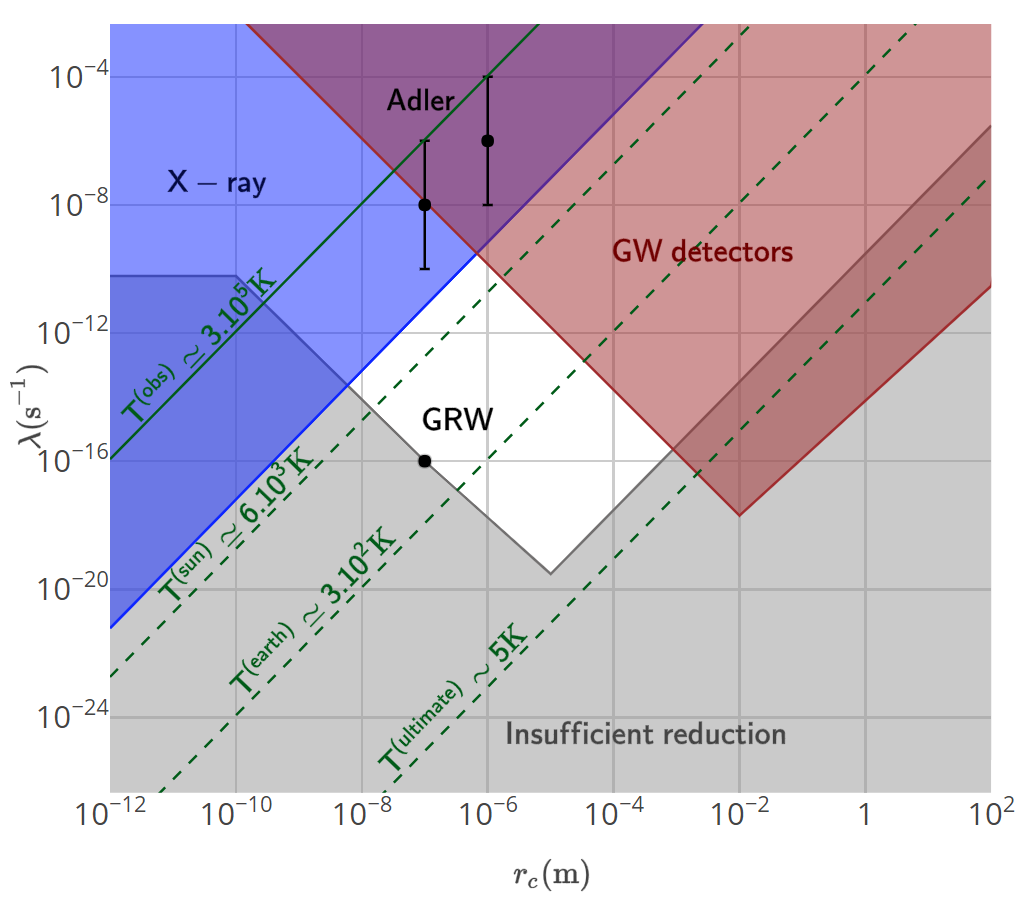
In future, the Large Synoptic Survey Telescope (LSST) will be able to image apparent magnitude objects Abell et al. 2009; at 5 pc, such objects have luminosity W, and a surface temperature of . Such an observation which would improve bounds on the CSL model, as shown in Fig. 1.
In the event that either DES or LSST fails to observe such objects, it would suggest either a (surprisingly) low local density of neutron stars, or that nearby neutron stars are unobservably cold (i.e. ). The latter inference would further rule out parts of the CSL parameter diagram, also shown in Fig. 1.
More speculatively, we might hope to one day be able to eliminate the possibility of an equilibrium temperature like that of our own planet, , which would falsify the historical GRW values by two orders of magnitude.
What might be the ultimate observable limit, even in principle? Neutron stars would be net thermal sources indefinitely if their minimum equilibrium temperature exceeded the cosmic microwave background (CMB) temperature. Though this would be difficult to observe terrestrially, it does offer an intriguing limit. Below , we find that the CSL parameter bounds are too low for collapse models to be effective, as shown in Fig. 1.
For the DP model, upper bounds on can be obtained if the model is required to provide a consistent theory of fundamental semiclassical gravity Tilloy and Diósi 2017. In this context, the regulator affects the Newtonian potential and the law of the gravitational force breaks down for . The Newtonian force is well measured for distances as short as Hagedorn 2015, which provides a conservative upper bound, m. Even supposing cold neutron stars of a few Kelvin, we find m. Hence the range of values allowed for the DP model could not (even in principle) be closed by the temperature of neutron stars alone, and gravitational upper bounds would need to be improved in parallel.
On the other hand, refinements and extensions of the CSL model with colored noise (cCSL) Bassi and Ghirardi 2002; Adler and Bassi 2007, dissipation (dCSL) Smirne et al. 2014, or both Ferialdi and Bassi 2012, containing additional parameters (such as a high frequency cutoff or a temperature) are known to yield weaker heating effects. Consequently, the constraints we put forward here would be weaker for these models.
In summary, with a conservative estimate of neutron star cooling based on the currently observed coldest neutron stars, one obtains constraints on the CSL model (albeit weaker than from spontaneous X-ray emission studies) and on the DP model (m, competitive with state of the art gravitational wave interferometer data). Improving the observational upper bound on neutron star equilibrium temperatures would yield substantial improvements. If we could measure an old, cold neutron star one could test more of the CSL parameter diagram. This motivates a systematic survey of nearby, cold neutron stars.
Acknowledgements.
We thank Philip Pearle and Tamara Davis for helpful discussions during development of this work. AT was supported by the Alexander von Humboldt foundation. TMS was supported by the Australian Research Council Centre of Excellence for Engineered Quantum Systems CE170100039.References
- Pearle (1989) P. Pearle, Phys. Rev. A 39, 2277 (1989).
- Ghirardi et al. (1990) G. C. Ghirardi, P. Pearle, and A. Rimini, Phys. Rev. A 42, 78 (1990).
- Bassi and Ghirardi (2003) A. Bassi and G. Ghirardi, Phys. Rep. 379, 257 (2003).
- Bassi et al. (2013) A. Bassi, K. Lochan, S. Satin, T. P. Singh, and H. Ulbricht, Rev. Mod. Phys. 85, 471 (2013).
- Diósi (1987) L. Diósi, Phys. Lett. A 120, 377 (1987).
- Penrose (1996) R. Penrose, Gen. Relativ. Gravit. 28, 581 (1996).
- Gisin (1989) N. Gisin, Helv. Phys. Acta 62, 363 (1989).
- Wiseman and Diósi (2001) H. Wiseman and L. Diósi, Chem. Phys. 268, 91 (2001).
- Ghirardi et al. (1986) G. C. Ghirardi, A. Rimini, and T. Weber, Phys. Rev. D 34, 470 (1986).
- (10) Note that the factor in eq. 6 has also been fixed to in the literature.
- Tilloy and Diósi (2016) A. Tilloy and L. Diósi, Phys. Rev. D 93, 024026 (2016).
- Tilloy and Diósi (2017) A. Tilloy and L. Diósi, Phys. Rev. D 96, 104045 (2017).
- Diósi (1990) L. Diósi, Phys. Rev. A 42, 5086 (1990).
- Pearle (1999) P. Pearle, Phys. Rev. A 59, 80 (1999).
- Tumulka (2006) R. Tumulka, J. Stat. Phys. 125, 821 (2006).
- Bedingham (2011) D. J. Bedingham, Found. Phys. 41, 686 (2011).
- Pearle (2015) P. Pearle, Phys. Rev. D 91, 105012 (2015).
- Tilloy (2017) A. Tilloy, arXiv:1702.06325 (2017).
- Juárez-Aubry et al. (2018) B. A. Juárez-Aubry, B. S. Kay, and D. Sudarsky, Phys. Rev. D 97, 025010 (2018).
- Pearle and Squires (1994) P. Pearle and E. Squires, Phys. Rev. Lett. 73, 1 (1994).
- Bahrami (2018) M. Bahrami, Phys. Rev. A 97, 052118 (2018).
- Adler and Vinante (2018) S. L. Adler and A. Vinante, Phys. Rev. A 97, 052119 (2018).
- Laloë et al. (2014) F. Laloë, W. J. Mullin, and P. Pearle, Phys. Rev. A 90, 052119 (2014).
- Lattimer et al. (1994) J. M. Lattimer, K. A. van Riper, M. Prakash, and M. Prakash, Astrophysical journal 425, 802 (1994).
- Lattimer and Prakash (2001) J. M. Lattimer and M. Prakash, The Astrophysical Journal 550, 426 (2001).
- Yakovlev and Pethick (2004) D. Yakovlev and C. Pethick, Annual Review of Astronomy and Astrophysics 42, 169 (2004), https://doi.org/10.1146/annurev.astro.42.053102.134013 .
- Keane et al. (2013) E. F. Keane, M. A. McLaughlin, M. Kramer, B. W. Stappers, C. G. Bassa, M. B. Purver, and P. Weltevrede, ApJ 764, 180 (2013).
- Carlesso et al. (2016) M. Carlesso, A. Bassi, P. Falferi, and A. Vinante, Phys. Rev. D 94, 124036 (2016).
- Helou et al. (2017) B. Helou, B. J. J. Slagmolen, D. E. McClelland, and Y. Chen, Phys. Rev. D 95, 084054 (2017).
- Piscicchia et al. (2017) K. Piscicchia, A. Bassi, C. Curceanu, R. D. Grande, S. Donadi, B. C. Hiesmayr, and A. Pichler, Entropy 19, 7 (2017).
- Toros et al. (2017) M. Toros, G. Gasbarri, and A. Bassi, Phys. Lett. A 381, 3921 (2017).
- Adler (2007) S. L. Adler, J. Phys. A: Math. Theor. 40, 2935 (2007).
- Drlica-Wagner et al. (2018) A. Drlica-Wagner, I. Sevilla-Noarbe, E. S. Rykoff, R. A. Gruendl, B. Yanny, D. L. Tucker, B. Hoyle, A. C. Rosell, G. M. Bernstein, K. Bechtol, M. R. Becker, A. Benoit-Lévy, E. Bertin, M. C. Kind, C. Davis, J. de Vicente, H. T. Diehl, D. Gruen, W. G. Hartley, B. Leistedt, T. S. Li, J. L. Marshall, E. Neilsen, M. M. Rau, E. Sheldon, J. Smith, M. A. Troxel, S. Wyatt, Y. Zhang, T. M. C. Abbott, F. B. Abdalla, S. Allam, M. Banerji, D. Brooks, E. Buckley-Geer, D. L. Burke, D. Capozzi, J. Carretero, C. E. Cunha, C. B. D’Andrea, L. N. da Costa, D. L. DePoy, S. Desai, J. P. Dietrich, P. Doel, A. E. Evrard, A. F. Neto, B. Flaugher, P. Fosalba, J. Frieman, J. García-Bellido, D. W. Gerdes, T. Giannantonio, J. Gschwend, G. Gutierrez, K. Honscheid, D. J. James, T. Jeltema, K. Kuehn, S. Kuhlmann, N. Kuropatkin, O. Lahav, M. Lima, H. Lin, M. A. G. Maia, P. Martini, R. G. McMahon, P. Melchior, F. Menanteau, R. Miquel, R. C. Nichol, R. L. C. Ogando, A. A. Plazas, A. K. Romer, A. Roodman, E. Sanchez, V. Scarpine, R. Schindler, M. Schubnell, M. Smith, R. C. Smith, M. Soares-Santos, F. Sobreira, E. Suchyta, G. Tarle, V. Vikram, A. R. Walker, R. H. Wechsler, and J. Z. and, The Astrophysical Journal Supplement Series 235, 33 (2018).
- Sartore, N. et al. (2010) Sartore, N., Ripamonti, E., Treves, A., and Turolla, R., A&A 510, A23 (2010).
- Abell et al. (2009) P. A. Abell et al. (LSST Science, LSST Project), (2009), arXiv:0912.0201 [astro-ph.IM] .
- Hagedorn (2015) C. A. Hagedorn, A Sub-Millimeter Parallel-Plate Test of Gravity, Ph.D. thesis, University of Washington (2015).
- Bassi and Ghirardi (2002) A. Bassi and G. Ghirardi, Phys. Rev. A 65, 042114 (2002).
- Adler and Bassi (2007) S. L. Adler and A. Bassi, J. Phys. A: Math. Theor. 40, 15083 (2007).
- Smirne et al. (2014) A. Smirne, B. Vacchini, and A. Bassi, Phys. Rev. A 90, 062135 (2014).
- Ferialdi and Bassi (2012) L. Ferialdi and A. Bassi, Phys. Rev. A 86, 022108 (2012).
Supplementary material
We compute the power generated by spontaneous collapse for a generic continuous Markovian non-dissipative collapse model and then evaluate the result for the CSL and DP models.
We consider a rather generic non-relativistic Hamiltonian for fermions with:
| (12) | ||||
| (13) |
where and are the local anti-commuting creation / annihilation operators and we neglect spin. We note that commutes with the local mass density and thus does not contribute to . Introducing such that we have:
| (14) |
We shall prove that:
| (15) |
where is the total number of neutrons. Let us compute the first commutator using the canonical anti-commutation relations and evaluate the integral:
| (16) | ||||
| (17) | ||||
| (18) |
Upon insertion in the second commutator, the first term in (18) will vanish. Using again the canonical anti-commutation relations we get:
| (19) |
Once integrated over , the first term will be proportional to by symmetry, and thus will not contribute. Using on the second term we get:
| (20) |
In this integration by part, we have neglected boundary terms which would vanish once applied to a density matrix sufficiently well behaved at infinity (which is reasonable for a compact object). As before, the gradient of evaluated in vanishes and we are left with:
| (21) |
Carrying the final integration over yields as advertised:
| (22) |
For the CSL model, we have:
| (23) | ||||
| (24) |
Hence:
| (25) |
Finally, for the CSL model, this gives:
| (26) |
which depends on the quantum state only through the total number of particles.
For the DP model, the regularized kernel can easily be evaluated in Fourier space:
| (27) | ||||
| (28) |
hence:
| (29) | ||||
| (30) |
and
| (31) |