Two-stage Circular-circular Regression with Zero-inflation: Application to Medical Sciences
Jayant Jha∗ Prajamitra Bhuyan† 11
1
Both authors contributed equally to this paper.
∗Institut de Neurosciences des Systèmes, Aix-Marseille University, Marseille
†Department of Mathematics, Imperial College London, London
Keywords: Abnormal gait, Astigmatism, Latent variable, Metropolis-Hastings algorithm, Rose diagram, Truncated wrapped Cauchy.
Abstract
This paper considers the modeling of zero-inflated circular measurements concerning real case studies from medical sciences. Circular-circular regression models have been discussed in the statistical literature and illustrated with various real-life applications. However, there are no models to deal with zero-inflated response as well as a covariate simultaneously. The Möbius transformation based two-stage circular-circular regression model is proposed, and the Bayesian estimation of the model parameters is suggested using the MCMC algorithm. Simulation results show the superiority of the performance of the proposed method over the existing competitors. The method is applied to analyse real datasets on astigmatism due to cataract surgery and abnormal gait related to orthopaedic impairment. The methodology proposed can assist in efficient decision making during treatment or post-operative care.
1 Introduction
In many real-world experiments, measurements are taken in angles, and such variables are commonly labeled as ‘circular variables’ or ‘directional variables’ in the statistics literature (Mardia and Jupp, 2000). The need for developing statistical methods to study circular regression is important due to its wide application in various fields of science, e.g., orthopaedics (Jammalamadaka and SenGupta, 2001, p-4), meteorology (Kato et al., 2008), ecology (Fisher and Lee, 1992), and geoscience (Rivest, 1997). Sarma and Jammalamadaka, 1993 proposed a generic circular-circular regression by joint modeling of the sine and cosine of the angular response on the trigonometric polynomial function of the angular covariate. In this context, some rotational models have been proposed where the predicted mean direction of the response is a fixed rotation of the covariate. See Mackenzie, 1957 and Rivest, 1997 for more details. Bhattacharya and Sengupta, 2009 proposed a Bayesian hierarchical framework for linear–circular regression. Downs and Mardia, 2002 proposed the Möbius transformation based regression link function for circular-circular regression to analyze the relationships between the peak systolic blood pressure times on different days, and wind directions at two different times. Later, Kato et al., 2008 also considered the Möbius transformation based link function by reparameterizing the model of Downs and Mardia, 2002 and applied this model to study the association between the spawning time of fish and the time of low tide. Other applications of the Möbius transformation based circular-circular regression model in opthalmology and genetics are discussed in Jha and Biswas, 2018 and Rueda et al., 2015, respectively. In this article, we consider the problem of modeling circular measurements motivated by the following case studies from orthopaedics and ophthalmology.
1.1 Abnormal Gait Data
The ability to walk safely and efficiently is essential for an independent and productive life. Gait disorders lead to a loss of personal freedom, and increased risk of injuries that result in a marked reduction in the quality of life (Mahlknecht et al., 2013). In the last couple of decades, due to the increased awareness of the importance of gait control, researchers across the globe focused their research programs on the clinical and therapeutic aspects of walking and balance (Nutt et al., 2011). Orthopaedic impairments of the lower extremities are the most common reasons for non-neurological gait disorders in adults (Mahlknecht et al., 2013). Patients with gait disorders caused by orthopaedic impairments are often referred to a physical therapist for treatment. Therapists visually observe the patient’s gait to determine effective treatment protocol or evaluate the effect of a therapeutic intervention. Various kinematic features like sagittal plane angular movements (flexion-extension) at the ankle and knee are extremely important in determining abnormal gait Therapists visually observe the patient’s gait to determine effective treatment protocol or evaluate the effect of a therapeutic intervention. Various kinematic features like sagittal plane angular movements (flexion-extension) at the ankle and knee are extremely important in determining abnormal gait(Jammalamadaka et al., 1986). Bio-engineers are interested to analyse the interlimb coordination concerning the flexion-extension to make an efficient design for the body-powered knee-ankle prosthesis (Ingraham et al., 2016). The human walking cycle consists of a period when the foot is on the ground, followed by the next phase of the forward movement known as swing. Recent research suggests that the ankle extensors provide necessary kinetic energy for the initiation of swing (Jessop and Pain, 2016). However, there is a lack of knowledge about the biomechanical process, which leads to the high power output of the ankle extensors (Lipfert et al., 2014). In this article, we consider a study conducted at the Bio-Engineering Unit, University of Calcutta, on a total of 29 individuals, including 10 healthy persons and 19 patients with unilateral orthopaedic impairment. Measurements on ankle and knee flexion-extension were recorded using electrogoniometers while subjects were walking at their own pace along an 8-meter long walkway turning around at each end. Previous research found no statistically significant difference between the motions of the right and left limb of a healthy person. Therefore, the angular movements of patient’s healthy limb can be used for comparison with the affected side in the presence of orthopaedic impairments (Roaas and Andersson, 1982). The principal objective of this study is to assess the recovery of orthopaedic patients and compare their gait with that of a healthy person.
1.2 Cataract Surgery Data
A cataract is a clouding that develops in the natural lens of the eye or its envelope. In due course of time, the lens loses its transparency and leads to partial or total loss of vision. This has been documented to be the most significant cause of bilateral blindness in India (Thulasiraj et al., 2003; Murthy et al., 2008a; Mohan, 1989). Cataract surgery is the removal of the opaque natural lens from the eye, and an artificial intra-ocular lens implant is then inserted to restore vision. India is a signatory to the World Health Organization resolution on VISION 2020: The Right to Sight. Efforts from all stakeholders have resulted in an increased number of cataract surgeries performed in India (Murthy et al., 2008b). It is well-known that one common side effect of the cataract surgery is that the incision causes unwanted changes to the natural corneal shape causing an astigmatic eye. The refractive error of the astigmatic eye induces several focal points in different directions. For example, the image may be perfectly focused on the retina in the horizontal (sagittal) plane, but not in the vertical (tangential) plane. There are two types of astigmatism based on the axes of the principal meridians - regular or irregular. In this paper, we consider regular astigmatism, where the principal meridians are perpendicular. For regular astigmatism, its axis ranges from to . In general, regular astigmatism can be subdivided into three types: (i) With-the-rule astigmatism (WTR) - the vertical meridian () is steepest (e.g. an American football lying on its side), (ii) Against-the-rule astigmatism (ATR)- the horizontal meridian () is steepest (e.g. an American football standing on its end), and (iii) Oblique astigmatism - the steepest curve lies in or (Morlet et al., 2001; Mimouni et al., 2017). The eye affected by WTR astigmatism sees vertical lines more sharply than horizontal lines. The situation is reversed for ATR astigmatism. Oblique astigmatism is worse than WTR and ATR astigmatism because most of the standard objects (e.g. letters) in our surroundings are horizontal or vertical. The objects get distorted horizontally or vertically for WTR and ATR astigmatism, whereas the distortion is severe for oblique astigmatism. The visual distortions for different types of astigmatism are displayed in Figure 1. It is of primary interest for ophthalmologists to study post-operative astigmatism and visual recovery over time (Zheng et al., 1997). In this article, we consider a study conducted at Disha Eye Hospital and Research Center, Barrackpore, West Bengal, India, over a period of two years (2008-10). In total, 54 patients were operated, and the axes of astigmatism were measured on the 1st, 7th, and 15th days after the surgery. See Bakshi, 2010 for a detailed description of the study and data description. The main objective of regular monitoring is to study the process of visual recovery and identify patients who require additional care to minimize post-operative trauma. In particular, medical practitioners are interested in foreseeing the improvement of patients based on previous inspections.

1.3 The challenge in analysing Cataract Surgery and Abnormal Gait Data
There are some critical issues involved in the modeling of astigmatism data under consideration. According to medical practitioners, if the axis is closer to , or , then it is not a matter of serious concern as most of the standard objects in nature are horizontal or vertical. Therefore, it is preferred that the axis is closer to , or . In order to make only one preferred direction, the observed angles are multiplied with 4 and then transformed by taking mod . Consequently, the preferred angle reduces to ( ) and hence, the multimodal distribution becomes a distribution having a single mode at . The effect of this transformation on circular distribution is illustrated in Figure 2. In this particular study, the measurements were taken up to the precision of . Therefore, the transformed variables become zero-inflated due to the high concentration of observations censored in the interval . The transformed axes of astigmatism after 7 days and 15 days of the surgery are presented using circular plots in Figure 3. A similar issue arises related to the measurements on ankle extension in abnormal gait data. The measurements were taken up to the precision of and averaged over strides of each individual. Almost of the observations on healthy individuals, and of the observations on orthopaedically impaired patients, are recorded as .

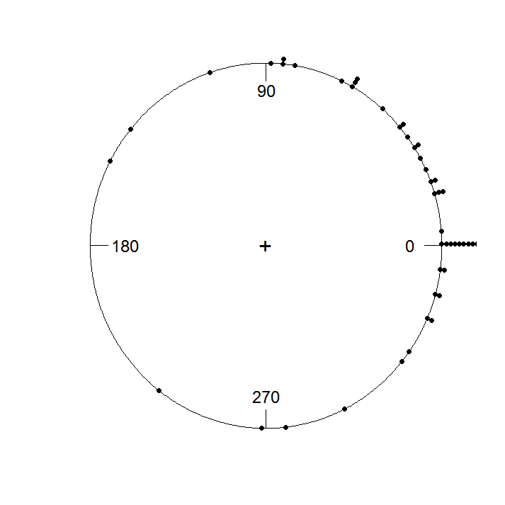

Numerous studies focusing on zero-inflated random variables in the linear setup are available in the literature. Tobin, 1958, Heckman, 1974 (Heckman, 1974, Heckman, 1979) proposed some models in the context of linear regression where the responses are zero-inflated. Lambert, 1992 considered Poisson regression for count data with excess zeros in the response variable. Bhuyan et al., 2019 discussed the case when both the responses and covariates are zero-inflated and proposed estimation methodology under a Bayesian setup. See Min and Agresti, 2002 for a detailed review of the zero-inflated regression models. However, in all of these works, the response and the covariate are linear in nature, where zero-inflation is caused by censorship through a selection mechanism. The case of circular random variables is considerably different from linear ones. The difference mainly arises due to the topology of the circle, where the zero cannot be considered to be located at the boundary of the sample space. In this context, a spike at zero may be interpreted in the same way as a spike at any other angle, since the origin can be fixed arbitrarily without loss of generality. There are only a few works on the analysis of zero-inflated circular data in the literature. The modeling of a circular random variable with point-accumulation was studied in Biswas et al., 2016. In the context of circular-circular regression, Jha and Biswas, 2018 proposed a model with a zero-inflated response variable and discussed the associated inferential issues. However, there is no model available in the literature for the case of a zero-inflated circular covariate. To avoid such difficulty, Jha and Biswas, 2018 analysed a subset of the dataset, considering only non-zero covariate values. It is important to note that the conventional circular-circular regression model and the model proposed by Jha and Biswas, 2018 are not appropriate for handling excess zeros in the covariate, and provide biased results. Moreover, the existing models are not capable of joint modeling of the periodical observations on astigmatism recorded over three different inspections. To model such data, we propose a two-stage circular-circular regression model based on continuous latent variables. In contrast to the assumption of randomly occurring zeros in Jha and Biswas, 2018, we consider a more realistic assumption that zero inflation occurs due to censoring. In Section 2, we discuss the modeling approach and propose an estimation methodology under a Bayesian setup using the Markov chain Monte Carlo (MCMC) algorithm. Some generalisations and a special case of the proposed model are also discussed in the same section. The performance of the proposed method is compared with the existing competitors through simulation in Section 3. Analysis of real datasets on post-operative astigmatism and abnormal gait are presented in Section 4. The key findings are summarised and concluded with some discussions on future research in Section 5.
2 Proposed Model and Methodology

In this section, we first describe the Möbius transformation based circular-circular regression model proposed by Kato et al., 2008, which is a reparameterization of the model proposed by Downs and Mardia, 2002. This reparameterization induces a nice geometry to the regression link function. When the angular error follows wrapped Cauchy distribution, it provides some advantages in terms of distributional properties as the wrapped Cauchy distribution is closed under rotation and Möbius transformation. See Kato et al., 2008 for details. It is important to note that the rotational model proposed by Mackenzie, 1957, where the predicted mean direction of the response is a fixed rotation of the covariate, is a special case of the Möbius transformation based model. Unlike the rotational model, this model is also appropriate when there is a high concentration of observed responses on a section of the unit circle. This unique feature makes the model parameters easily interpretable and provides interesting insights.
Let us represent circular random variables and as complex random variables and , respectively taking values on the circumference of a unit circle. The circular-circular regression model of Kato et al., 2008 is represented as:
| (1) |
where , , , and the angular error follows a wrapped Cauchy distribution with mean direction . The regression link function, which is a form of Möbius transformation, is a mapping from a unit circle onto itself. Here, is the rotation parameter because the multiplication by a unit complex number is an anti-clockwise rotation by the argument of the same unit complex number. In this case, the predicted mean given is obtained by rotating by , where is the intersection of the unit circle with the line joining and (see Figure 4). For , the regression link function can be geometrically represented as a straight line connecting and . Therefore, it also covers the cases in which the predicted mean direction depends on the conjugate of (i.e. when there is a reflection of ). The intersection of this line with the unit circle is then rotated by to obtain the predicted mean direction . If is closer to 1 and is uniformly distributed, then is highly concentrated around . The distribution of becomes independent of if . For , the predicted mean direction is just a rotation of , i.e. . See Kato et al., 2008 for more details.
To model the axis of astigmatism recursively based on three consecutive inspections, we extend the circular-circular regression model (1) in a two-stage setup as:
| (2) |
| (3) |
where , , , ; , , , and . We assume for , where represents the wrapped Cauchy distribution with parameters and . Also, and are assumed to be independently distributed. In the literature of Econometrics, is known as instrumental variable (Cameron and Trivedi, 2005, p-97), which may not directly effect the response but it can induce changes only through the covariate . This modeling approach allows us to compare the visual recovery of the patients over two consecutive weeks.
Note that the circular-circular regression model, given by equation (1), is inadequate for handling zero-inflated data (Jha and Biswas, 2018). Similarly, the aforementioned two-stage model will give very poor fit to the data due to point accumulation at zero for both the response and the covariate. In order to model zero-inflated circular data, we first define circular latent variables and as
and
respectively, where , are constants taking values in . Now we propose the two-stage circular-circular regression model based on the aforementioned latent variables as
| (4) |
| (5) |
where , , , . In the absence of instrumental variable, one can still use (4) and (5) for modeling of zero-inflated response and covariate with . Note that the above model reduces to the two-stage circular-circular regression model without zero-inflation, given by (2) and (3), when .
2.1 Bayesian Estimation
We propose a Bayesian estimation of the model parameters involved in the two-stage model given by (4) and (5), using the MCMC algorithm based on data augmentation. In the conventional frequentist approach, computational challenges arise in the model fitting due to intractable numerical integration involved in the log-likelihood function. Unlike the usual frequentist set-up, the proposed Bayesian approach provides simultaneous estimation of the model parameters and a natural framework for prediction over unobserved data. Thus, by generating posterior predictive densities, rather than point estimates, we can make probability statements giving greater flexibility in presenting results. For instance, we can discuss findings concerning specific hypotheses or in terms of credible intervals which can offer a more intuitive understanding for the practitioners.
Let us denote the observed data by , and the parameter vector by for , where , , , , . Also, denote the density of the wrapped Cauchy distribution and the truncated wrapped Cauchy distribution by and , respectively, where . The joint posterior density of the model parameters and the latent variable involved in equation (4) is given by
where , and denotes the prior density of . Similarly, the joint posterior density of the model parameters and the latent variable involved in equation (5), is given by
where , and denotes the prior density of . The full conditional densities of the latent variables and have the following closed-form expressions
| (6) |
and
| (7) |
respectively. We propose an algorithm for generating samples from the truncated wrapped Cauchy distribution which is discussed in Subsection 2.2. The full conditional densities of the model parameters and are given by
| (8) |
| (9) |
respectively. Note that the full conditionals of and cannot be expressed in closed form. Therefore, we employ the Metropolis-Hastings algorithm for generating samples from the posterior densities of the parameters and the detailed algorithm is provided in Subsection 2.2. In our context, and are known a priori. However, in many situations, these are not known and one can consider a suitable prior as discussed in Subsection 2.2.
2.2 Sampling Algorithms
2.2.1 Sample Generation from Truncated Wrapped Cauchy Distribution
Let be a circular random variable following truncated wrapped Cauchy distribution with pdf , where . The support of is , if , and , otherwise. To generate samples from , for , we simulate observations from and accept the observations which lie in . Similarly, for , we accept the observations lying in . However, the acceptance rate is very low for small values of . For example, the acceptance rate is approximately when , , , and . Thus, we propose a novel algorithm for generating samples from the truncated wrapped Cauchy distribution based on the geometry of the Möbius transformation.
If is uniformly distributed in and , then follows wrapped Cauchy distribution with parameters , and , where (Kato et al., 2008). The geometry of the transformation is presented in Figure 4 with , and . Note that, is the point on the circumference of the unit circle which is situated at the intersection of the line joining and and the unit circle. It is easy to see that follows wrapped Cauchy distribution with and . To simulate an observation from the truncated wrapped Cauchy distribution, first generate a unit complex number uniformly in the region between and where and . Then, consider the argument of its inverse Möbius transformation as . This construction is diagrammatically illustrated in Figure 5 and summarized in a simple algorithm below.
Algorithm 1: Sampling from Truncated Wrapped Cauchy Distribution
- Step 1:
Take , and choose a point in the support of .
- Step 2:
Generate a random unit complex number uniformly from the arc joining and containing , where .
- Step 3:
Take .

2.2.2 Metropolis-Hastings Algorithm
For the purpose of Bayesian estimation, we consider the following prior distributions for the parameter vectors and . The joint prior distribution can be expressed as the product of , , and , for . It can be easily verified that the joint posterior density is proper for . Similar priors have been considered by Ravindran and Ghosh, 2011 in the context of circular-circular and circular-linear regressions. For the purpose of implementing Metropolis-Hastings Algorithm, we consider the proposal distributions for to be uniform, and the proposal distributions for are chosen to be exponential. As discussed before, and may be unknown and one can employ the following MCMC algorithm with priors and , and uniform proposal densities.
Algorithm 2: Metropolis Hastings Algorithm
- Step 1:
- Step 2:
Generate the model parameters sequentially from the corresponding proposal densities and denote it as . Given the previous value of and the current draw , return with probability
where denotes the proposal density at with parameter , and denotes the full conditional densities given by equations (8) and (9). Otherwise, repeat the previous value .
- Step 3:
Repeat Step 1 and Step 2 until convergence.
2.3 Special case
Under certain restrictions on the model parameters, the geometry of the Möbius transformation based link function provides interesting insights when there is a preferred direction for the response variable. Without loss of generality, we consider to be the preferred direction. Then, we consider a special case of the circular-circular regression model given by equation (1), where and . Under this restriction, the symmetry about the preferred direction for the predicted responses and the corresponding covariate values is maintained as . This can be seen directly from the geometry as shown in Figure 4 by taking and . In this case, the larger the value of , the more is the tendency of the predicted response to move towards . The constraint ensures that both the predicted mean direction and the corresponding covariate value lie on the same semi-circle having the diameter as the line segment joining and . This implies that the predicted mean direction lies on the shortest arc joining the respective covariate value and when . This special case also ensures that , for all , where . That is, the closer the covariate value is to , the closer is the corresponding predicted mean response to .
This special case can be reparameterized and presented as the centered regression model proposed by Downs and Mardia, 2002 with both the angular location parameters fixed at 0. The corresponding regression link function can be written as , where . As the angular parameters are fixed at 0, there is a one-one monotonic correspondence between and , given by . Therefore, the parameter , if greater than or less than 1, indicates the general tendency of the predicted response to move towards or away from as compared to its covariate value, respectively.
For the two-stage circular-circular regression model given by equations (4) and (5), we consider , and . As compared to the unrestricted model, this special case enforces all the predicted response to either move towards or away from zero as compared to its respective covariate value. Therefore, the two stages of the regression model can be compared in terms of their tendency to move towards on the basis of the posterior distributions of and . In contrast to the general model, we consider uniform prior and proposal distributions for and . The choices of prior and proposal distributions for all the other parameters are considered same as discussed in Subsection 2.2.2. When there is a preferred direction, it is easier to compare two regression models based on the estimates obtained from the special case as compared to Model I. This special case is parsimonious and easy to interpret. However, a drawback of this special case as compared to the unrestricted model is that all the predicted mean responses simultaneously move towards or away from the preferred direction. Therefore, this model is not appropriate for prediction when some of the observed responses are closer, and some are farther from the preferred direction compared to their respective covariate values. We consider this special case for data analysis to provide some insights into the cataract surgery data based on the posterior distributions of the model parameters.
2.4 Some Generalisations
The proposed two-stage model, given by (4) and (5), can be extended to the case when there are multiple circular covariates. Jha and Biswas, 2017 proposed a multiple circular-circular regression model (MCR2) based on Möbius transformation which is represented as:
| (10) |
where , , for for , and are covariates. Note that the model (10) reduces to (1) for . Now, without loss of generality, we consider that is a zero-inflated covariate and define a latent circular variable as:
where . Note that the the response is also zero-inflated and we consider the latent response as defined in Section 2. Then, the generalised two-stage circular-circular regression model for zero-inflated data with multiple covariates is given as:
and
where , , , for , , , and are covariates used to regress . For the purpose of Bayesian estimation, one can consider Dirichlet priors for and with parameter vectors and , respectively. The priors for , for , and for , can be taken as uniform. The MCMC algorithm mentioned in Subsection 2.2 is readily extended to this generalised model. Further, one can generalise the proposed model for modeling data with multiple points of accumulation due to asymmetric censoring intervals.
3 Simulation Studies
In order to study the performance of the proposed method, we generate data considering different choices of parameter values for two different sample sizes, 50 and 100. We generate from von Mises distribution with mean 0 and concentration parameter . The five different sets of parameters values of and are chosen, keeping radians (), such that the approximate proportions of zeros in the response and covariate are given by , , , and , respectively. We consider the priors as discussed in the Subsection 2.2 with for . We generate 100,000 samples from the posterior distributions of the associated model parameters using the MCMC algorithm and find the posterior mean and standard deviation of the linear parameters based on every 10th iterate discarding the first 40,000 iterations as burn-in. Similarly, we compute the posterior circular mean and circular dispersion for the circular parameters. This is repeated 500 times and the average estimates are reported in Tables 1-5. Note that, the circular dispersion (c.d.) for circular observations is given by , where and for each . We also report the coverage probability (CP) corresponding to all the parameters. As expected, the standard deviation (s.d.) and c.d. decrease as the sample size increases (See Tables 1-5). In this limited simulation study, our proposed method seems to perform reasonably well.
| n=50 | |||||||
|---|---|---|---|---|---|---|---|
| Parameters | circular mean (c.d.) | Bias | CP | Parameters | mean (s.d.) | Relative Bias | CP |
| -0.019(0.193) | -0.019 | 0.71 | 0.907(0.083) | 0.008 | 0.90 | ||
| 0.019(0.128) | 0.019 | 0.74 | 1.177(0.100) | -0.019 | 0.92 | ||
| 0.020(0.208) | 0.020 | 0.70 | 0.845(0.030) | -0.006 | 0.95 | ||
| -0.018(0.110) | -0.018 | 0.75 | 0.846(0.030) | -0.005 | 0.95 | ||
| n=100 | |||||||
| Parameters | circular mean (c.d.) | Bias | CP | Parameters | mean (s.d.) | Relative Bias | CP |
| -0.003(0.061) | -0.003 | 0.77 | 0.903(0.058) | 0.003 | 0.91 | ||
| -0.004 (0.038) | -0.004 | 0.76 | 1.192(0.055) | 0.007 | 0.91 | ||
| 0.002(0.066) | 0.002 | 0.77 | 0.847(0.022) | -0.004 | 0.92 | ||
| 0.003(0.031) | 0.003 | 0.76 | 0.848(0.020) | -0.002 | 0.95 | ||
| n=50 | |||||||
|---|---|---|---|---|---|---|---|
| Parameters | circular mean (c.d.) | Bias | CP | Parameters | mean (s.d.) | Relative Bias | CP |
| 0.025(0.198) | 0.025 | 0.71 | 1.177(0.127) | -0.019 | 0.90 | ||
| -0.017(0.114) | -0.017 | 0.77 | 1.183(0.087) | -0.014 | 0.91 | ||
| -0.023(0.180) | -0.023 | 0.71 | 0.843(0.030) | -0.008 | 0.95 | ||
| 0.014(0.098) | 0.014 | 0.78 | 0.844(0.030) | -0.007 | 0.95 | ||
| n=100 | |||||||
| Parameters | circular mean (c.d.) | Bias | CP | Parameters | mean (s.d.) | Relative Bias | CP |
| -0.005(0.044) | -0.005 | 0.79 | 1.189(0.080) | -0.009 | 0.93 | ||
| -0.011 (0.046) | -0.011 | 0.76 | 1.190(0.056) | -0.008 | 0.94 | ||
| 0.005(0.039) | 0.005 | 0.78 | 0.847(0.021) | -0.004 | 0.95 | ||
| 0.012(0.038) | 0.012 | 0.76 | 0.847(0.020) | -0.004 | 0.95 | ||
| n=50 | |||||||
|---|---|---|---|---|---|---|---|
| Parameters | circular mean (c.d.) | Bias | CP | Parameters | mean (s.d.) | Relative Bias | CP |
| -0.025(0.127) | -0.025 | 0.79 | 0.888(0.078) | -0.013 | 0.91 | ||
| 1.552(0.087) | -0.019 | 0.77 | 1.448(0.122) | -0.034 | 0.88 | ||
| 0.025(0.138) | 0.025 | 0.80 | 0.843(0.030) | -0.008 | 0.95 | ||
| 0.016(0.062) | 0.016 | 0.79 | 0.844(0.031) | -0.007 | 0.93 | ||
| n=100 | |||||||
| Parameters | circular mean (c.d.) | Bias | CP | Parameters | mean (s.d.) | Relative Bias | CP |
| -0.060(0.022) | -0.060 | 0.86 | 0.894(0.034) | -0.007 | 0.93 | ||
| 1.587 (0.030) | 0.016 | 0.78 | 1.481(0.082) | -0.013 | 0.91 | ||
| 0.059(0.024) | 0.059 | 0.88 | 0.846(0.021) | -0.005 | 0.93 | ||
| -0.013(0.021) | -0.013 | 0.77 | 0.847(0.021) | -0.004 | 0.93 | ||
| n=50 | |||||||
|---|---|---|---|---|---|---|---|
| Parameters | circular mean (c.d.) | Bias | CP | Parameters | mean (s.d.) | Relative Bias | CP |
| 1.543(0.075) | 0.028 | 0.72 | 0.897(0.086) | -0.003 | 0.92 | ||
| 0.009(0.095) | 0.009 | 0.81 | 1.441(0.116) | -0.039 | 0.90 | ||
| 0.029(0.165) | 0.029 | 0.75 | 0.844(0.031) | -0.007 | 0.95 | ||
| -0.009(0.070) | -0.009 | 0.81 | 0.841(0.031) | -0.011 | 0.95 | ||
| n=100 | |||||||
| Parameters | circular mean (c.d.) | Bias | CP | Parameters | mean (s.d.) | Relative Bias | CP |
| 1.532(0.060) | -0.039 | 0.76 | 0.897(0.056) | -0.037 | 0.91 | ||
| 0.008 (0.027) | 0.008 | 0.83 | 1.484(0.083) | -0.011 | 0.91 | ||
| 0.041(0.061) | 0.041 | 0.76 | 0.847(0.021) | -0.004 | 0.95 | ||
| -0.008(0.019) | -0.008 | 0.83 | 0.847(0.021) | -0.004 | 0.94 | ||
| n=50 | |||||||
|---|---|---|---|---|---|---|---|
| Parameters | circular mean (c.d.) | Bias | CP | Parameters | mean (s.d.) | Relative Bias | CP |
| 1.559(0.012) | -0.025 | 0.95 | 0.303(0.049) | 0.010 | 0.94 | ||
| 1.572(0.001) | 0.009 | 0.94 | 0.318(0.044) | 0.060 | 0.95 | ||
| 0.030(0.013) | 0.030 | 0.96 | 0.842(0.031) | -0.009 | 0.95 | ||
| 0.007(0.037) | 0.007 | 0.94 | 0.847(0.030) | -0.004 | 0.94 | ||
| n=100 | |||||||
| Parameters | circular mean (c.d.) | Bias | CP | Parameters | mean (s.d.) | Relative Bias | CP |
| 1.567(0.002) | -0.004 | 0.93 | 0.301(0.032) | 0.003 | 0.92 | ||
| 1.568 (0.006) | -0.003 | 0.93 | 0.308(0.029) | 0.027 | 0.93 | ||
| 0.003(0.003) | 0.003 | 0.94 | 0.847(0.020) | -0.004 | 0.95 | ||
| 0.004(0.016) | 0.004 | 0.91 | 0.848(0.019) | -0.002 | 0.97 | ||
| Model I | |||||||
|---|---|---|---|---|---|---|---|
| Parameters | circular mean (c.d.) | Bias | CP | Parameters | mean (s.d.) | Relative Bias | CP |
| 0.073(0.004) | 0.003 | 0.56 | 0.898(0.060) | -0.002 | 0.91 | ||
| 0.063(0.001) | -0.007 | 0.47 | 1.186(0.057) | -0.012 | 0.90 | ||
| -0.002(0.011) | -0.002 | 0.57 | 0.928(0.010) | -0.077 | 0.94 | ||
| -0.002(0.008) | -0.002 | 0.44 | 0.949(0.008) | -0.001 | 0.95 | ||
| Model II | |||||||
| Parameters | circular mean (c.d.) | Bias | CP | Parameters | mean (s.d.) | Relative Bias | CP |
| 0.092(0.006) | 0.022 | 0.54 | 0.894(0.064) | -0.007 | 0.88 | ||
| 0.036(0.001) | -0.034 | 0.09 | 1.019(0.010) | -0.151 | 0.08 | ||
| -0.046(0.007) | -0.046 | 0.55 | 0.922(0.011) | -0.084 | 0.92 | ||
| -0.029(0.001) | -0.029 | 0.10 | 0.990(0.003) | 0.042 | 0.17 | ||
| Model III | |||||||
| Parameters | circular mean (c.d.) | Bias | CP | Parameters | mean (s.d.) | Relative Bias | CP |
| 0.088(0.004) | 0.018 | 0.55 | 0.899(0.057) | -0.001 | 0.89 | ||
| 0.037(0.001) | -0.033 | 0.10 | 1.016(0.009) | -0.153 | 0.05 | ||
| -0.020(0.005) | -0.020 | 0.55 | 0.928(0.011) | -0.077 | 0.96 | ||
| -0.031(0.001) | -0.031 | 0.09 | 0.991(0.003) | 0.043 | 0.14 | ||
| Model I | |||||||
|---|---|---|---|---|---|---|---|
| Parameters | circular mean (c.d.) | Bias | CP | Parameters | mean (s.d.) | Relative Bias | CP |
| 0.075(0.003) | 0.005 | 0.51 | 0.901(0.064) | 0.001 | 0.90 | ||
| 0.060(0.001) | -0.010 | 0.48 | 1.170(0.053) | -0.025 | 0.83 | ||
| -0.018(0.004) | -0.018 | 0.51 | 0.934(0.010) | 0.004 | 0.92 | ||
| -0.002(0.001) | -0.002 | 0.48 | 0.955(0.007) | 0.005 | 0.84 | ||
| Model II | |||||||
| Parameters | circular mean (c.d.) | Bias | CP | Parameters | mean (s.d.) | Relative Bias | CP |
| 0.061(0.003) | -0.009 | 0.47 | 0.912(0.057) | 0.013 | 0.79 | ||
| 0.035(0.001) | -0.035 | 0.02 | 1.005(0.003) | -0.163 | 0.01 | ||
| -0.033(0.004) | -0.033 | 0.46 | 0.937(0.010) | 0.008 | 0.82 | ||
| -0.033(0.001) | -0.033 | 0.02 | 0.998(0.001) | 0.051 | 0.02 | ||
| Model III | |||||||
| Parameters | circular mean (c.d.) | Bias | CP | Parameters | mean (s.d.) | Relative Bias | CP |
| 0.056(0.003) | -0.014 | 0.46 | 0.911(0.057) | 0.011 | 0.87 | ||
| 0.035(0.001) | -0.035 | 0.02 | 1.005(0.009) | -0.163 | 0.00 | ||
| -0.003(0.004) | -0.003 | 0.48 | 0.935(0.011) | 0.005 | 0.90 | ||
| -0.033(0.001) | -0.033 | 0.02 | 0.998(0.003) | 0.051 | 0.03 | ||
| Model I | |||||||
|---|---|---|---|---|---|---|---|
| Parameters | circular mean (c.d.) | Bias | CP | Parameters | mean (s.d.) | Relative Bias | CP |
| 0.065(0.002) | -0.005 | 0.51 | 0.919(0.067) | 0.021 | 0.87 | ||
| 0.056(0.001) | -0.014 | 0.51 | 1.141(0.051) | -0.049 | 0.72 | ||
| -0.016(0.003) | -0.016 | 0.51 | 0.940(0.009) | 0.011 | 0.73 | ||
| -0.007(0.001) | -0.007 | 0.51 | 0.961(0.007) | 0.012 | 0.61 | ||
| Model II | |||||||
| Parameters | circular mean (c.d.) | Bias | CP | Parameters | mean (s.d.) | Relative Bias | CP |
| 0.055(0.001) | -0.015 | 0.33 | 0.950(0.040) | 0.056 | 0.54 | ||
| 0.034(0.001) | -0.036 | 0.00 | 1.002(0.001) | -0.165 | 0.00 | ||
| -0.044(0.001) | -0.044 | 0.34 | 0.963(0.008) | 0.035 | 0.39 | ||
| -0.033(0.001) | -0.033 | 0.00 | 0.999(0.001) | 0.052 | 0.00 | ||
| Model III | |||||||
| Parameters | circular mean (c.d.) | Bias | CP | Parameters | mean (s.d.) | Relative Bias | CP |
| 0.061(0.002) | -0.009 | 0.52 | 0.924(0.063) | 0.027 | 0.84 | ||
| 0.033(0.001) | -0.037 | 0.00 | 1.002(0.001) | -0.165 | 0.00 | ||
| -0.011(0.003) | -0.011 | 0.50 | 0.941(0.009) | 0.012 | 0.70 | ||
| -0.032(0.001) | -0.032 | 0.00 | 0.999(0.001) | 0.052 | 0.00 | ||
3.1 Model Comparison and Sensitivity Analysis
For the purpose of comparison, we consider three different models, Model I, Model II and Model III, given by (4) and (5), (2) and (3), and (4) and (3), respectively. Note that Model I accounts for zero-inflation in both the response and the covariate, however, Model II does not account for zero-inflation, and Model III accounts for zero-inflation in the response only. We first compare the performance of parameter estimates associated with Model I, Model II and Model III when the data is generated from Model I with sample size and radians (). We consider the priors as discussed in the Subsection 2.2 with for . The averages of the estimates over 500 replications are reported in Table 6. It is observed that the performance of most of the estimates based on Model II and Model III are biased compared to those of Model I. The estimates of the parameters associated with the regression of on based on Model II and Model III have large bias and very low CP. It is important to note that the estimates associated with the regression of on based on Model III, which incorporates zero-inflation in the response, are biased compared to those of Model I that also incorporates zero-inflation in the covariate. These observations clearly indicate that both Model II and Model III are inadequate to model the underlying relationship in the data when there is significant zero-inflation in both response and covariate.
In order to carry out a sensitivity analysis, we consider a misspecified simulation model, where and are first generated as before and then contaminated with randomly occurring zeros with probability . Note that the aforementioned model reduces to the proposed two-stage circular-circular regression model, given by (4)-(5), for . We generate data of sample size for two different choices of with , and compare the different models with respect to bias and CP based on 500 replications. The results are presented in Table 7 and 8. It is observed that the performance of the estimates for all the models deteriorate with respect to both bias and CP as increases. The bias and CP for most of the parameters based on Model I are considerably better compared to Model II and III. In particular, the CP of the parameters associated with the regression of on based on Model II and Model III are close to zero. Even with the higher value of , the estimates obtained from Model I are robust compared to those of Model II and Model III.
Next, we compare the run-time of different models per dataset in Table 9, under the simulation settings presented in Tables 6-8, using a computer equipped with 32 GB RAM and 2.59 GHz Intel Core(TM) i7-8850H processor. As expected, the computing time increases with the increase in the proportion of zeros for Model I and Model III. We also observed the same pattern for the simulation settings corresponding to Tables 1-5. The difference among the run-times for the three different models is less than 3 minutes, even with large proportion of zeros. As it turns out, Model I seems to have an edge concerning the trade-off between computational time and model performance in presence of zero-inflation.
| Model I | Model II | Model III | |
|---|---|---|---|
| Table 6 | 6.75 | 4.95 | 5.01 |
| Table 7 | 6.95 | 4.82 | 5.81 |
| Table 8 | 7.66 | 5.21 | 5.95 |
4 Case Studies
As discussed before, applications of circular-circular regression are commonly found in the domain of orthopaedics and ophthalmology. In this Section, we consider two different case studies from each of these application areas. Significant amount of zero-inflation is observed in both ‘Cataract Surgery Data’ and ‘Abnormal Gait Data’. The results from analysis of these datasets based on the proposed methodology along with the practical implications are discussed below.
4.1 Analysis of Cataract Surgery Data
As discussed in Section 1, we consider a dataset on astigmatism observed at three different inspections from a study on cataract surgery conducted at Disha Eye Hospital and Research Center. In the proposed two-stage setup, we first consider the response () and the covariate () as the axis of astigmatism after 15 days and 7 days of the surgery, respectively. Among the 54 observations, there are and zeros in response and covariate, respectively. In this study, measurements on the axis of astigmatism just after a day of the surgery are also available. Next, we model the axis of astigmatism after 7 days of the surgery () with covariate as the axis of astigmatism just after a day of surgery (). In order to apply the methodology provided in Section 2, we consider radians () and for . This particular choice of and is considered as the original axes of astigmatism are censored in the interval .
We generate 250,000 samples from the posterior distributions of the associated model parameters using the MCMC algorithm and find the posterior mean/circular mean and s.d./c.d. based on every 10th iterate discarding the first 70,000 iterations as burn-in. The convergence of the chains is monitored graphically and using Geweke’s diagnostic test after taking cosine transformation of the samples for the circular parameters. The mean/circular mean, s.d/c.d. of the parameters and the results for Geweke’s diagnostic test are reported in Appendix A of the Supplementary Material. We also report the highest posterior density (HPD) credible interval. The algorithm for finding the HPD credible interval for circular parameters is provided in Jha, 2017. As expected, the HPD credible interval for both and does not contain 1. This indicates that and are dependent on and , respectively.
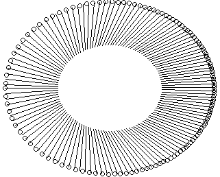
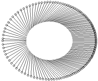
In order to compare the recovery processes in consecutive weeks, we present spoke plots in Figure 6 and Figure 7 based on the estimates from Model I and its special case, respectively. In the spoke plots, the predicted axes of astigmatism in the outer circle are joined with the corresponding axes of astigmatism a week before in the inner circle. It is important to note that there is a preferred direction for the axis of astigmatism, and it makes practically more sense to consider the equivalence of symmetric points about . It can be seen from the spoke plots based on Model I (See Figure 6), that the predicted responses for symmetric observations around are not symmetric. For example, the predicted mean direction for is rotated towards , while for , it is rotated away from . However, for the special case, the symmetric points rotate symmetrically towards the preferred direction (See Figure 7). Hence, the equivalence with respect to the preferred direction is maintained. Also, the predicted axes of astigmatism in the second week (astigmatism at day 15 based on day 7) are more attracted towards than those of the first week (astigmatism at day 7 based on day 1) for both the models. This indicates that the recovery in the second week is more than the recovery in the first week. This finding is also supported by the fact that , based on the estimates obtained from the special case of Model I.
Medical practitioners are more interested in identifying patients whose performances either improve or deteriorate. For this purpose, we consider Model I and compute the posterior predictive distributions of the axis of astigmatism at day 15 and day 7 with three different initial conditions fixed at (normal), (intermediate), and (serious) on day 1. We also compute the posterior predictive distribution of the axis of astigmatism at day 15 based on those three initial conditions on day 7. In Figure 8, we present rose diagrams based on the aforementioned posterior predictive distributions to analyse the recovery of patients over time. In all the cases, it is seen that the predictive distribution is concentrated around if the initial axis of astigmatism is close to (See the top panel of Figure 8). For both intermediate and serious cases, improvement is more prominent in the second week compared to the first week as the posterior predictive distribution shifts more towards in the second week (See middle and bottom panel of Figure 8). For the serious case, the patients who show early sign of recovery improve more at the end of two weeks than those with delayed recovery (See second and third column at the bottom panel in Figure 8).
To compare the predicted values with the observed values, we convert the predicted values in degrees and round off to the nearest integer divisible by 4. In general, the patients not affected by astigmatism after 7 days of the surgery remain unaffected in the near future. In this dataset, 17 patients remain unaffected by astigmatism during the study period and the fitted model identifies all of them correctly. We detect the improvement in 17 out of the 21 patients. However, the deterioration is detected for only 6 out of the 13 patients. Therefore, one can conclude that the patients whose conditions have improved and seem to stay good in the future require less monitoring while the rest of the patients need more frequent monitoring and care.


| Astigmatism at day 7 on day 1 | Astigmatism at day 15 on day 1 | Astigmatism at day 15 on day 7 | |
|---|---|---|---|
 |
 |
 |
Initial axis |
 |
 |
 |
Initial axis |
 |
 |
 |
Initial axis |
4.2 Analysis of Abnormal Gait Data
We consider a study on gait control conducted at Bio-Engineering Unit, University of Calcutta. The objective of this study is to analyse the angular movements of the patient’s affected limb with that of a healthy person while keeping the angular movement of the healthy limb fixed at a specified level within the range of natural variation. For this purpose, we consider the response () and the covariate () as the angle of ankle extension of the affected and the unaffected legs, respectively, of the 19 individuals with unilateral orthopaedic impairment. We also jointly model the angle of ankle extension of the non-dominated leg () as the response with that of the dominated leg () as covariate based on the measurements taken from 10 healthy individuals. As mentioned before, more than of the observations are recorded as in both response and covariate. For the purpose of joint modeling, we consider a shared-parameter model replacing with in (4), where , and takes value for orthopaedically impaired individuals, and , otherwise. In order to apply the methodology provided in Section 2, we consider , and radians (). We generate 150,000 samples from the posterior distributions of the associated model parameters using the MCMC algorithm and discard the first 50,000 iterations as burn-in. Here also, no convergence issues are found based on Geweke’s diagnostic test. The parameter estimates along with HPD credible interval are reported in Appendix A of the Supplementary Material.
Based on the results, it can be seen from Figure 9 that even the confidence ellipse of the posterior distribution of contains . This indicates that the rotation model is sufficient to explain the regression for this particular dataset under consideration. To study the difference between healthy and orthopaedically impaired person, we plot the posterior density of in Figure 10. It is clearly visible that the bulk of the distribution is near 0. This is also supported from Figure 11, and by the fact that HPD credible interval of includes (see Appendix A of the Supplementary Material). This indicates that the angle of ankle extension of the affected leg of an orthopaedically impaired patient is not significantly different from that of the non-dominating leg of a healthy person when the angle of extension of the other leg are fixed at the same level. Moreover, the HPD credible interval of also contains zero, which indicates no significant difference between the angles of ankle extension for both legs for healthy individuals as well as the orthopaedically impaired patients. This is also visible from the posterior predictive distributions of the angle of ankle extension of the affected/non-dominating leg where the modes of the posterior predictive distributions are very close to the respective angle of extension of the healthy/dominating leg (see Figure 12).

5 Discussion
In this paper, a Bayesian methodology has been developed for a circular-circular regression model with point-accumulation in covariate and response, unlike the existing frequentist methods that only model the cases with point-accumulation in the response variable. Circular-circular regression is not well studied from a Bayesian perspective. This paper makes an attempt in that direction and possibly for the first time Bayesian estimation is proposed for the Möbius transformation based circular-circular regression model. The proposed method is applied to analyse two real datasets on post operative astigmatism and abnormal gait due to orthopaedic impairments. Our analysis provides interesting insights and predictions associated with the recovery of patients. Findings from the analysis of cataract surgery data may help to reduce post-operative trauma and improve the patient’s experience after cataract surgery. Similarly, bio-engineers can exploit the analytical findings from abnormal gait data to develop efficient prosthesis.
In general, the methodology is applicable for conventional circular-circular regression with or without point-accumulation in response and/or covariate. Also, one can implement the proposed methodology with other choices of link function and/or choices of angular error distributions. As the latent variables involved in the modeling are continuous, one can easily modify the proposed methodology for a discrete response variable with multiple points of accumulation. Therefore, the scope of the proposed method goes far beyond the particular case studies under consideration. For example, one can model wind direction data where the recorded measurements are among some pre-specified discrete directions (e.g. North, West, East, and South). Although we have not considered missing data in our current analysis, a simple data augmentation technique has to be incorporated into the proposed methodology when the missingness is ignorable. Another possible direction of future research is to develop a bias-reduced estimation methodology for zero-inflated circular-circular regression using the approach proposed by Schwartz and Giles, 2016. In some real-life scenarios, a circular response may depend on both linear and circular covariates. It will be an interesting problem to model such data and develop associated estimation methodology. As the Möbius transformation based circular-circular regression model is not readily extendable to the case with linear covariates, it can be considered as future work.
Acknowledgement
The work of Dr. Prajamitra Bhuyan was supported in part by the Lloyd’s Register Foundation programme on data-centric engineering at the Alan Turing Institute, UK. The authors are thankful to Prof. Anup Dewanji, Dr. Arnab Chakraborty, Prof. Debasis Sengupta, Dr. Jayabrata Biswas, Dr. Sourabh Bhattacharya, and Mr. Sudipta Kundu for many helpful comments and suggestions.
References
- Bakshi, (2010) Bakshi, P. (2010). Evaluation of various surgical techniques in Brunescent cataracts. Unpublished thesis, Disha Eye Hospital, India.
- Bhattacharya and Sengupta, (2009) Bhattacharya, S. and Sengupta, A. (2009). Bayesian analysis of semiparametric linear-circular models. Journal of Agricultural, Biological, and Environmental Statistics, 9:14–33.
- Bhuyan et al., (2019) Bhuyan, P., Biswas, J., Ghosh, P., and Das, K. (2019). A bayesian two-stage regression approach of analyzing longitudinal outcomes with endogeneity and incompleteness. Statistical Modelling, 19(2):157–173.
- Biswas et al., (2016) Biswas, A., Jha, J., and Dutta, S. (2016). Modelling of circular random variables with a spike at zero. Statistics and Probability Letters, 109:194–201.
- Cameron and Trivedi, (2005) Cameron, A. C. and Trivedi, P. K. (2005). Microeconometrics: Methods and Applications. Cambridge University Press.
- Downs and Mardia, (2002) Downs, T. D. and Mardia, K. V. (2002). Circular regression. Biometrika, 89:683–697.
- Fisher and Lee, (1992) Fisher, N. I. and Lee, A. J. (1992). Regression models for an angular response. Biometrika, 48:665–677.
- Heckman, (1974) Heckman, J. (1974). Shadow prices, market wages and labor supply. Econometrica, 42:679–694.
- Heckman, (1979) Heckman, J. (1979). Sample selection bias as a specification error. Journal of the Royal statistical Society, Series B, Methodological, 49:127–145.
- Ingraham et al., (2016) Ingraham, K. A., Fey, N. P., Simon, A. M., and Hargrove, L. J. (2016). Assessing the relative contributions of active ankle and knee assistance to the walking mechanics of transfemoral amputees using a powered prosthesis. PLoS One.
- Jammalamadaka et al., (1986) Jammalamadaka, S. R., Bhadra, N., Charurvedi, D., Kutty, T. K., Mujumder, P. P., and Poduval, G. (1986). Functional assessment of knee and ankle during level walking. In T. Krishnan, editor, Data Analysis in Life Science, Indian Statistical Institute, Calcutta, India., pages 21–54.
- Jammalamadaka and SenGupta, (2001) Jammalamadaka, S. R. and SenGupta, A. (2001). Topics in Circular Statistics. World Scientific Publishing Co. Pte. Ltd.
- Jessop and Pain, (2016) Jessop, D. M. and Pain, M. T. (2016). Maximum velocities in flexion and extension actions for sport. Journal of Human Kinetics., 50:37–44.
- Jha, (2017) Jha, J. (2017). Best approach direction for spherical random variables. Technical Report No. ASU/2017/5, Applied Statistics Unit, Indian Statistical Institute, Kolkata, URL: http://www.isical.ac.in/ asu/TR/TechRepASU201705.pdf.
- Jha and Biswas, (2017) Jha, J. and Biswas, A. (2017). Multiple circular-circular regression. Statistical Modelling, 17(3):142–171.
- Jha and Biswas, (2018) Jha, J. and Biswas, A. (2018). Circular-circular regression model with a spike at zero. Statistics in Medicine, 37(1):71–81.
- Kato et al., (2008) Kato, S., Shimizu, K., and Shieh, G. S. (2008). A circular-circular regression model. Statistica Sinica, 18:633–645.
- Lambert, (1992) Lambert, D. (1992). Zero-inflated poisson regression, with an application to defects in manufacturing. Technometrics, 34:1–14.
- Lipfert et al., (2014) Lipfert, S. W., Günther, M., Renjewski, D., and Seyfarth, A. (2014). Impulsive ankle push-off powers leg swing in human walking. Journal of Experimental Biology., 217:1218–1228.
- Mackenzie, (1957) Mackenzie, J. K. (1957). The estimation of an orientation relationship. Acta Crystallographica, 10:61–62.
- Mahlknecht et al., (2013) Mahlknecht, P., Kiechl, S., Bloem, B. R., Willeit, J., Scherfler, C., Gasperi, A., Rungger, G., Poewe, W., and Seppi, K. (2013). Prevalence and burden of gait disorders in elderly men and women aged 60-97 years: a population-based study. PLoS One, 8(7).
- Mardia and Jupp, (2000) Mardia, K. V. and Jupp, P. E. (2000). Directional Statistics. Wiley, London.
- Mimouni et al., (2017) Mimouni, M., Nemet, A., Pokroy, R., Sela, T., Munzer, G., and Kaiserman, I. (2017). The effect of astigmatism axis on visual acuity. European Journal of Ophthalmology, 27:308–311.
- Min and Agresti, (2002) Min, Y. and Agresti, A. (2002). Modeling nonnegative data with clumping at zero: A survey. Journal of Iranian Statistical Society, 1:7–33.
- Mohan, (1989) Mohan, M. (1989). National survey of blindness-india. NPCB-WHO Report. New Delhi: Ministry of Health and Family Welfare, Government of India.
- Morlet et al., (2001) Morlet, N., Minassian, D., and Dart, J. (2001). Astigmatism and the analysis of its surgical correction. British Journal of Ophthalmology, 85:1127–1138.
- (27) Murthy, G. V., Gupta, S., Ellwein, L. B., Munoz, S. R., Bachani, D., and Dada, V. K. (2008a). A population-based eye survey of older adults in a rural district of rajasthan: I. central vision impairment, blindness, and cataract surgery. Ophthalmology, 108(4):679–85.
- (28) Murthy, G. V. S., Gupta, S. K., John, N., and Vashist, P. (2008b). Current status of cataract blindness and vision 2020: The right to sight initiative in india. Indian Journal of Ophthalmology, 56(6):489–494.
- Nutt et al., (2011) Nutt, J. G., Horak, F. B., and Bloem, B. R. (2011). Milestones in gait, balance, and falling. Movement Disorders, 26(6):1166–1174.
- Ravindran and Ghosh, (2011) Ravindran, P. and Ghosh, S. K. (2011). Bayesian analysis of circular data using wrapped distributions. Journal of Statistical Theory and Practice, 5(4):547–561.
- Rivest, (1997) Rivest, L. P. (1997). A decentred predictor for circular-circular regression. Biometrika, 84:318–324.
- Roaas and Andersson, (1982) Roaas, A. and Andersson, G. B. J. (1982). Normal range of motion of the hip, knee and ankle joints in male subjects, 30-40 years of age. Acta Orthopaedica Scandinavica., 53(2):205–208.
- Rueda et al., (2015) Rueda, C., Fernandez, M. A., Barragan, S., Mardia, K. V., and Peddada, S. D. (2015). Circular piecewise regression with an application to cell-cycle biology. Biometrics, 64:1–20.
- Sarma and Jammalamadaka, (1993) Sarma, Y. and Jammalamadaka, S. (1993). Circular regression. Proceeding of the Third Pacific Area Statistical Conference. VSP: Utrecht, Netherlands., pages 109–128.
- Schwartz and Giles, (2016) Schwartz, J. and Giles, D. E. (2016). Bias-reduced maximum likelihood estimation of the zero-inflated poisson distribution. Communications in Statistics - Theory and Methods, 45(2):465–478.
- Thulasiraj et al., (2003) Thulasiraj, R., Nirmalan, P. K., Ramakrishnan, R., Krishnadas, R., Manimekalai, T. K., Baburajan, N., Katz, J., Tielsch, J. M., and Robin, A. L. (2003). Blindness and vision impairment in a rural south indian population: the aravind comprehensive eye survey. Ophthalmology, 110(8):1491–1498.
- Tobin, (1958) Tobin, J. (1958). Estimation of relationships for limited dependent variables. Econometrica, 26:24–36.
- Zheng et al., (1997) Zheng, L., Merriam, J. C., and Zaider, M. (1997). Astigmatism and visual recovery after ‘large incision’ extracapsular cataract surgery and ‘small’ incisions for phakoemulsification. Transactions of the American Ophthalmological Society, 95:387–415.