Pair Dispersion in Dilute Suspension of Active SwimmersPreprint: AIP/123-QED
Abstract
Ensembles of biological and artificial microswimmers produce long-range velocity fields with strong nonequilibrium fluctuations, which result in dramatic increase diffusivity of embedded particles (tracers). While such enhanced diffusivity may point to enhanced mixing of the fluid, a rigorous quantification of the mixing efficiency requires analysis of pair dispersion of tracers, rather than simple one–particle diffusivity. Here, we calculate analytically the scale-dependent coefficient of relative diffusivity of passive tracers embedded in a dilute suspension of run-and-tumble microswimmers. Although each tracer is subject to strong fluctuations resulting in large absolute diffusivity, the small-scale relative dispersion is suppressed due to the correlations in fluid velocity which are relevant when the inter-tracers separation is below the persistence length of the swimmers motion. Our results suggest that the reorientation of swimming direction plays an important role in biological mixing and should be accounted in design of potential active matter devices capable of effective fluid mixing at microscale.
Suspensions of swimming microorganisms, a prototype of non-equilibrium, exhibit fascinating behaviors distinct from their equilibrium counterparts. Even at dilute concentrations, active swimmers can produce large non-Gaussian fluctuations in fluid velocity with long-range/time correlations, and not constrained by the fluctuation-dissipation theorem Rushkin_2010; Kurihara_2017; Chen_2007; Underhill_2011. The swimmer-induced hydrodynamic fluctuations have been shown to significantly enhance diffusivity of passive tracers placed in active suspensions Wu_2000; Leptos_2009; Wilson_2011; Kurtuldu_2011; Jepson_2013; Mino_2013. This observation is relevant to transport of nutrients, and may be relevant to understanding features of bacterial swimming Katija_2012. The enhanced tracer diffusion, driven either by motile organisms or by artificial self-propelled particles, can potentially be used for efficient mixing in microfluidic devices Kim_2004; Kim_2007.
But, does the enhanced diffusivity of tracers in active suspensions actually result in high mixing efficiency? Diffusive transport and mixing/stirring are often (and in some cases mistakenly, in our opinion) used interchangeably. Whereas the former is quantified by the one-particle diffusivity, the latter is associated with the relative dispersion of initially nearby tracers. Here we analytically investigate the effect of swimmer-induced hydrodynamic fluctuations on pair dispersion in a dilute active suspension. Our analysis uncovers the relation between scale-dependent mixing properties and randomization of swimming direction via stochastic tumbling. If the intertracer separation is sufficiently large, compared to the persistence length of swimmer trajectories, the relative dispersion is determined by the absolute diffusivity as the distant tracers move in an uncorrelated manner. In contrast, on spatial scales below the swimmer persistence length, correlations in the fluid velocity fluctuations can not be neglected leading to weaker relative dispersion.
Consider two non-Brownian tracer particles moving along Lagrangian trajectories in the incompressible fluid flow produced by an ensemble of active swimmers, see Fig. 1a. Following the seminal work by Richardson Richardson_1926, who established the foundations of two-particle dispersion in hydrodynamic turbulence, we consider the diffusion equation for the probability density of finding the tracers at separation at time
| (1) |
in which the (scale dependent) diffusion coefficient is defined as
| (2) |
where represents the Eulerian longitudinal velocity difference along the direction of particle separation, and the angular brackets denote averaging over the statistics of flow fluctuations. We assume spatial homogeneity and isotropy of the suspension; implying that the relative diffusivity depends only on the absolute value of the separation vector. In addition, Eq. (1) assumes that the probability distribution is spherically symmetric. Furthermore, describing the advection of passive tracers by means of a diffusion equation is based on the important assumption that the random velocity field is short-range correlated in time. This assumption will be justified at the end of the article.

As shown in Refs. Batchelor_1953; Kraichnan_1966 (see Appendix A for the details), the diffusion coefficient defined in Eq. (2) can be written as
| (3) |
in terms of the scalar pair correlation function of the fluid velocity,
| (4) |
Equation (3) explicitly relates the scale dependencies of relative diffusivity and velocity correlations. One may expect that at sufficiently large separations , the term in the integrand of this equation can be neglected as correlations between velocity fluctuations experienced by distant tracers are almost absent. Then the coefficient of relative diffusion is simply twice the absolute diffusivity, which can far exceed its thermal value even for dilute suspensions. It is clear, however, that the small-scale dispersion must be less pronounced due to the correlations present in the flow. Indeed, as we will see below, the relative diffusivity vanishes as the interparticle separation goes to zero. What is the characteristic length scale associated with the scale-dependent diffusivity ? This is the central question of this work.
To calculate , we need to describe the statistics of the flow fluctuations created by the active swimmers. Since the Reynolds number associated with swimming at microscale is small Purcell_1977 (), the fluid motion is governed by the Stokes equation. For an autonomously moving neutrally buoyant swimmer, a propulsive force is balanced by the resistive drag so that the swimmer exerts no net force on the fluid. Then the velocity field produced by the swimmer far away from its surface is determined by the leading order dipole term in a multipole expansion. Noting that the near-field flow (where high order harmonics are relevant) is not universal, we will consider dipolar swimmers for simplicity. Then, the fluid velocity induced at by a swimmer with orientation placed in the origin is given by (see, e.g., Refs. Lauga_2009; Yeomans_2014)
| (5) |
where denotes the strength of the force dipole exerted by the swimmer on the fluid with viscosity . The short-distance cut-off required to regularize singularity at is of the order of the physical size of a swimmer’s body. The strength is positive for pushers and negative for pullers Lauga_2009.

In the Stokes regime, the total fluid velocity is given by the superposition of flow contributions from all swimmers present in the system, i.e. , where and indicate, correspondingly, the position and the orientation of the th swimmer, and is given by Eq. (5). (We consider only a dilute suspension in which interactions between swimmers can be neglected, and thus assume that they move independently from each other.) In a statistically stationary state, the swimmers are uniformly distributed in the fluid with a concentration and the probability distribution of the swimmer orientation vector is isotropic. Then the two-point correlation function of the fluid velocity defined in Eq. (4) can be written as (see Appendix C)
| (6) |
where denotes the probability density that after the time the swimmer will be in with orientation having started at with the initial swimming direction . Equation (6) is valid at the leading order in concentration , accounting for correlations between the positions and orientations of the same swimmer at different moments of time.
To proceed further we need to specify the model for the swimmer’s motion. Let us assume that each swimmer moves ballistically with constant speed and undergoes complete reorientation at the rate . The random reorientations mimic the run-and-tumble behavior of bacteria Berg_1993 (see Fig 1b). It is known that real run-and-tumble dynamics is characterized by quick but non-instantaneous tumbles and exhibits correlations between directions of subsequent runs. Moreover, the runs are not perfectly straight due to rotational diffusion. However, what is important for succeeding arguments is that the swimmer’s orientation stochastically changes with time, and the fine details of the particular reorientation mechanism are not significant. As such, we adopt the analytically tractable model of uncorrelated Poisson tumbling to illustrate the main idea. In this case, the propagator entering Eq. (6) satisfies the kinetic equation Schnitzer_1993
| (7) |
supplemented by the initial condition .
Equation (7) is equivalent to the Boltzmann equation for the Lorentz model of electron conduction Lorentz_1905. The exact analytical solution of this equation can be constructed in the Fourier-Laplace space as shown in Refs. Hauge_1970; Martens_2012 (see also Appendix B). After lengthy but straightforward calculations, Eq. (6) reduces to
| (8) |
The appealing simplicity of the above relation is due to the vanishing of the contribution from the last term on the right-hand-side of Eq. (7), see Appendix C for the details.
Using Eqs. (5) and (8), we obtain the one-point correlation function (see Appendix D)
| (9) |
while the two-point correlation function for is found to be (see Appendix E)
| (10) |
see Fig. 2 for the illustration. Equations (9) and (10) generalize the results of Refs. Underhill_2008; Zaid_2011 where the one-point correlator (in the case ) and the one-time correlator were derived for the dipolar swimmer model.
Finally, inserting Eqs. (9) and (10) into Eq. (3), and performing integration, one finds
| (11) |
where we have introduced the swimmer persistence length , which is assumed to be large compared to the swimmer’s size , and denotes the exponential integral.
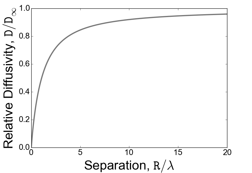
Equation (11) indicates that the relative diffusivity is a monotonically decreasing function of the interparticle separation, saturating to for , see Fig. 3. Estimating the strength of the force dipole as (see, e.g., Ref. Lauga_2009) we obtain where is the volume fraction of swimmers. Obviously, the limit of large separation corresponds to the uncorrelated motion of tracers so that is just twice the absolute diffusivity. Our estimate for is in agreement with previous studies of the hydrodynamic diffusion of non-Brownian tracers in dilute three-dimensional suspensions of dipolar swimmers with large persistence length (i.e. ) Lin_2011; Pushkin_2013; Kasyap_2014.
The small-scale asymptotic behavior of the relative diffusivity is linear, for . Equation (1) then implies a linear growth of the mean interparticle distance with time, , with
| (12) |
playing the role of a mean relative velocity. Estimated as , it is much smaller than the (rms) absolute tracer velocity as and by assumption. Despite of the enhanced diffusivity at the single particle level, nearby trajectories diverge relatively slowly due to the underlying velocity correlation. Indeed, the typical time it takes for two nearby fluid parcels to reach a separation of is given by , much longer than the naive estimate based on the assumption that the parcels undergo independent diffusive motions (as they do for ).
As was noted in the beginning of the article, describing dispersion by the diffusion equation is valid only when the fluid velocity fluctuations are short-range correlated in time. This is justified since the characteristic time associated with evolution of the separation vector accordingly to Eqs. (1) and (11) is large compared to the correlation time of a tracer’s relative velocity. Using Eqs. (9) and (10), the latter can be is estimated as for , while when . It is then evident that and and, therefore, the assumption of short correlation times is valid in both limits of small and large tracer separation.
Noteworthy, setting tumbling rate to zero we readily find from Eq. (11) that in the idealized system where swimmers move along infinite straight trajectories the relative diffusivity vanishes. This allows us to argue that independently on the particular mechanism underlying the randomization of the swimming direction, swimmer persistence length sets the boundary between two regimes of relative dispersion characterized by different mixing efficiencies. In particular, one may expect that mixing is always suppressed in the systems where swimmer reorientation occurs mainly upon hitting the container walls, since in this case the intertracer separation cannot be larger than the swimmer persistence length which is determined by the system size.
In conclusion, let us discuss some limitations of the analysis presented above, and possible directions for future studies. First, since we model the swimmer disturbance field as a point force dipole, our results cannot be directly applied to suspensions of quadrupolar swimmers such as active colloids and certain microorganisms Zottl_2016. Second, our analysis does not incorporate a detailed model of the near-field hydrodynamic interactions between the swimmer and the tracer particle. According to a recent experimental study of enhanced diffusion in a suspension of micro-alga Kasyap_2014, tracer entrainment by the near-flow of swimming microorganisms plays a crucial role in the physical regime when the tracer’s size is significantly smaller than that of the swimmers. Third, our model ignores Brownian motion, focusing on the purely convective transport of the tracers. This restricts applicability of the above results to the limit of large Peclet numbers, , where is the Brownian diffusivity of tracers. It may be possible to generalize calculation of the relative diffusivity beyond the assumptions and adopted here, based on recent theoretical progress Kasyap_2014; Burkholder_2017 in quantifying the absolute diffusivity. Fourth, here we focused on the very dilute regime neglecting any swimmer-swimmer correlations. However, a recent theoretical study Stenhammar_2017 indicates that, due to long-range nature of hydrodynamic interactions between swimmers, such correlations can become significant well below the onset of turbulence, resulting in non-linear scaling of the tracer diffusivity with swimmer concentration. Thus, further theoretical development is required to extend the present analysis to the case of moderate swimmer densities.
To summarize, we have characterized the spatio-temporal correlations present in a dilute suspension of run-and-tumble microswimmers by calculating the pair correlation function of the fluid velocity fluctuations. The knowledge of the two-point correlator allows us to derive an analytical expression for the relative diffusivity of passive tracers, thus, revealing those aspects of the mixing process that cannot be captured by the single-particle diffusivity. Our results provide insight into the role of swimmer tumbling (and other reorientation mechanisms) in bacteria-induced mixing in natural systems, and should be relevant to design of mixing enhancement systems using active swimmers.
Acknowledgements.
SB gratefully acknowledges support from the James S. McDonnell Foundation via its postdoctoral fellowship in studying complex systems. MK acknowledges support from NSF through grant DMR-1708280.Appendix A Relative diffusivity in incompressible random flow
Here we derive Eq. (3) for the relative diffusivity of passive tracers. The probability distribution of the separation vector of two tracers advected by short-time correlated incompressible random flow evolves accordingly to the diffusion equation
| (13) |
with the diffusivity tensor given by . If the flow is statistically homogeneous and isotropic, and the probability distribution is spherically symmetric, then Eq. (1) reduces to (see, e.g., Ref. Kraichnan_1966)
| (14) |
where is the longitudinal diagonal element of the diffusivity tensor in the coordinate system aligned with , which can be expressed as
| (15) | |||||
in terms of the scalar correlation function
| (16) |
and relaying on homogeneity and isotropy.
To derive Eq. (3) we note that the general form of the two-point velocity correlator in the homogeneous and isotropic random flow is given by (see Ref. Batchelor_1953)
| (17) |
where and are arbitrary functions of and . Let us also introduce the following scalar correlator
| (18) |
Here is the velocity component along an arbitrary chosen direction orthogonal to the separation vector . As it follows Eq. (17), the longitudinal and lateral velocity correlation functions, are , are related to the functions and as
| (19) | |||
| (20) |
and, therefore, Eq. (17) can be rewritten as
| (21) |
Next, the incompressibility condition, , implies that
| (22) |
where is the number of spatial dimensions, and consequently
| (23) |
The above equation allows us to express in terms of
| (24) |
Using Eqs. (21) and (24), we find
| (25) |
and, therefore,
| (26) |
Finally, inserting Eq. (26) into Eq. (15) one obtains
| (27) |
This expression gives Eq. (3) for . An equivalent representation of in terms of the energy-spectrum function (i.e. Fourier transform of ) can be found in Ref. Kraichnan_1966.
Appendix B Propagator of the run-and-tumble swimmer
Here we construct the solution to Eq. (7) by exploiting the trick proposed in Ref. Hauge_1970. It is convenient to use the spherical system of coordinates to parametrize the orientation vector . Then , where is the polar angle, and Eq. (7) from the main text can be written as
| (28) |
After the Fourier-Laplace transform
| (29) |
we obtain
| (30) |
Let us integrate Eq. (30) over assuming that the polar angle is measured from the direction determined by the wave vector
| (31) |
This allows us to express
| (32) |
Substituting this expression into Eq. (30), one obtains
| (33) |
or, equivalently,
| (34) |
Appendix C Velocity correlation function in suspension of swimmers
In this section we derive Eqs. (6) and (8). To compute the velocity field of the fluid we need to sum the contributions produced by all swimmers
| (35) |
Here and are, respectively, the position and the orientation of the th swimmer, and is given by Eq. (5) in the main text. Then, the two-point correlation function of the velocity can be written as
| (36) |
It is easy to check that in the absence of correlations between the different swimmers, all terms with go to zero after integration. Therefore the leading contribution comes from the correlations between position and orientation of the same swimmer at different moments of time. Taking into account that all swimmers are identical, we then obtain
| (37) |
where we have dropped the label for the swimmer number. Next, simple implementation of the Bayes formula yields
| (38) |
The first term in the right hand side of the last equation represents the joint probability distribution of the swimmer position and orientation, i.e.
| (39) |
where is the steady-state probability distribution of swimmer orientation and (=) is the volume of the system. We used the fact that in the statistically stationary state the probability density of the swimmer’s position is uniform at all positions.
The second factor in the right hand side of Eq. (38) represents the probability density that after the time the swimmer will be in having the orientation provided it starts in with orientation , i.e.
| (40) |
From Eq. (37) together with Eqs. (38-40) one obtains Eq. (6) from the main text.
Next, using the Fourier-Laplace transform of and we can rewrite Eq. (6) as
| (41) |
where is the contour in the plane of the complex variable , is given by Eq. (34) and
| (42) |
Taking into account Eq. (34), we find
| (43) | |||||
To perform integration over the swimmer orientations we choose a spherical system of coordinates with the zenith direction parallel to the wave vector . Then the vector is parametrised by the angle variables and . Let us note that
| (44) | |||||
and, therefore, the second term in the rhs of Eq. (43) goes to zero after integration over or . Since this zero contribution comes from the last term on the right hand side of Eq. (7), and there are no other contributions associated with this term, we can ignore it from the very beginning, thus, passing to the simpler kinetic equation
| (45) |
which is exactly solvable and gives
| (46) |
Appendix D The one-point correlation function
Appendix E The two-point correlation function
References
- (1) I. Rushkin, V. Kantsler, and R. E. Goldstein, “Fluid velocity fluctuations in a suspension of swimming protists,” Physical review letters, 105(18), 188101 (2010).
- (2) T. Kurihara, M. Aridome, H. Ayade, I. Zaid, & D. Mizuno, “Non-Gaussian limit fluctuations in active swimmer suspensions,” Phys. Rev. E 95(3), 030601 (2017).
- (3) D. T. Chen, A. W. C. Lau, L. A. Hough, M. F. Islam, M. Goulian, T. C. Lubensky, and A. G. Yodh, “Fluctuations and rheology in active bacterial suspensions,” Phys. Rev. Let. 99(14), 148302 (2007).
- (4) P. T. Underhill, and M. D. Graham, “Correlations and fluctuations of stress and velocity in suspensions of swimming microorganisms,” Physics of Fluids 23(12), 121902 (2011).
- (5) X.-L. Wu and A. Libchaber, “Particle diffusion in a quasi two-dimensional bacterial bath,” Phys. Rev. Lett. 84, 3017 (2000).
- (6) K. C. Leptos, J. S. Guasto, J. P. Gollub, A. I. Pesci, and R. E. Goldstein, “Dynamics of enhanced tracer diffusion in suspensions of swimming eukaryotic microorganisms,” Phys. Rev. Lett. 103, 198103 (2009).
- (7) L. G. Wilson, V. A. Martinez, J. Schwarz-Linek, J. Tailleur, G. Bryant, P. N. Pusey, & W. C. Poon, “Differential dynamic microscopy of bacterial motility,” Phys. Rev. Lett., 106(1), 018101 (2011).
- (8) H. Kurtuldu, J. S. Guasto, K. A. Johnson, and J. P. Gollub, “Enhancement of biomixing by swimming algal cells in two-dimensional films,” Proceedings of the National Academy of Sciences 108(26), 10391-10395 (2011).
- (9) A. Jepson, V. A. Martinez, J. Schwarz-Linek, A. Morozov, & W. C. Poon, “Enhanced diffusion of nonswimmers in a three-dimensional bath of motile bacteria,” Phys. Rev. E 88(4), 041002 (2013).
- (10) G. L. Mino, J. Dunstan, A. Rousselet, E. Clement, and R. Soto, “Induced diffusion of tracers in a bacterial suspension: theory and experiments,” J. Fluid Mech. 729, 423-444 (2013).
- (11) K. Katija, “Biogenic inputs to ocean mixing,” Journal of Experimental Biology 215(6), 1040-1049 (2012).
- (12) M. J. Kim and K. S. Breuer, “Enhanced diffusion due to motile bacteria,” Phys. Fluids 16, L78 (2004).
- (13) M. J. Kim and K. S. Breuer, “Controlled mixing in microfluidic systems using bacterial chemotaxis,” Anal. Chem. 79, 955 (2007).
- (14) LF. Richardson, “Atmospheric diffusion shown on a distance-neighbour graph,” Proc. R. Soc. Lond. Ser. A 110:709–37 (1926).
- (15) G. K. Batchelor, “The theory of homogeneous turbulence,” (Cambridge University Press, New York, 1953) pp. 46-50.
- (16) R. H. Kraichnan, “Dispersion of particle pairs in homogeneous turbulence,” The Physics of Fluids 9(10), 1937-1943 (1966).
- (17) E. M. Purcell, ”Life at low Reynolds number,” American journal of physics 45(1), 3-11 (1977).
- (18) E. Lauga and T. R. Powers, “The hydrodynamics of swimming microorganisms,” Reports on Progress in Physics 72(9), 096601 (2009).
- (19) J. M. Yeomans, D. O. Pushkin, and H. Shum, “An introduction to the hydrodynamics of swimming microorganisms,” The European Physical Journal Special Topics 223(9), 1771-1785 (2014).
- (20) H. C. Berg, “Random walks in biology,” (Princeton University Press, 1993)
- (21) M. J. Schnitzer, “Theory of continuum random walks and application to chemotaxis,” Phys. Rev. E 48(4), 2553 (1993).
- (22) H. A. Lorentz, (1905). HA Lorentz, Arch. Neerl. 10, 336 (1905). Arch. Neerl., 10, 336.
- (23) E. H. Hauge, “Exact and Chapman-Enskog Solutions of the Boltzmann Equation for the Lorentz Model,” The Physics of fluids 13(5), 1201-1208 (1970).
- (24) K. Martens, L. Angelani, R. Di Leonardo, and L. Bocquet, “Probability distributions for the run-and-tumble bacterial dynamics: An analogy to the Lorentz model,” The European Physical Journal E: Soft Matter and Biological Physics 35(9), 1-6 (2012).
- (25) Z. Lin, J. L. Thiffeault, and S. Childress, “Stirring by squirmers,” Journal of Fluid Mechanics, 669, 167-177 (2011).
- (26) D. O. Pushkin and J. M. Yeomans, “Fluid mixing by curved trajectories of microswimmers,” Phys. Rev. Lett. 111(18), 188101 (2013).
- (27) P. T. Underhill, J. P. Hernandez-Ortiz, and M. D. Graham, “Diffusion and spatial correlations in suspensions of swimming particles,” Phys. Rev. Lett. 100(24), 248101 (2008).
- (28) I. M. Zaid, J. Dunkel, and J. M. Yeomans, “Lévy fluctuations and mixing in dilute suspensions of algae and bacteria,” Journal of The Royal Society Interface 8(62), 1314-1331 (2011).
- (29) T. V. Kasyap, D. L. Koch, and M. Wu, “Hydrodynamic tracer diffusion in suspensions of swimming bacteria,” Physics of Fluids 26(8), 081901 (2014).
- (30) A. Zöttl and H. Stark, “Emergent behavior in active colloids,” Journal of Physics: Condensed Matter 28(25), 253001 (2016).
- (31) R. Jeanneret, D. O. Pushkin, V. Kantsler, and M. Polin, “Entrainment dominates the interaction of microalgae with micron-sized objects,” Nature communications 7, 12518 (2016).
- (32) E. W. Burkholder and J. F. Brady, “Tracer diffusion in active suspensions,” Phys. Rev. E 95(5), 052605 (2017).
- (33) J. Stenhammar, C. Nardini, R. W. Nash, D. Marenduzzo, and A. Morozov, “Role of correlations in the collective behavior of microswimmer suspensions,” Phys. Rev. Lett. 119(2), 028005 (2017).