Supporting Information: Artificial Intelligence Assists Discovery of Reaction Coordinates and Mechanisms from Molecular Dynamics Simulations

Hendrik Jung Thanks: These authors contributed equally to this work. Affiliation: Department of Theoretical Biophysics, Max Planck Institute of Biophysics, 60438 Frankfurt am Main, Germany. Roberto Covino Thanks: These authors contributed equally to this work. Affiliation: Department of Theoretical Biophysics, Max Planck Institute of Biophysics, 60438 Frankfurt am Main, Germany. Gerhard Hummer Corresponding author: gerhard.hummer@biophys.mpg.de Affiliation: Department of Theoretical Biophysics, Max Planck Institute of Biophysics, 60438 Frankfurt am Main, Germany. Affiliation: Institute of Biophysics, Goethe University, 60438 Frankfurt am Main, Germany.

Abstract

Exascale computing holds great opportunities for molecular dynamics (MD) simulations. However, to take full advantage of the new possibilities, we must learn how to focus computational power on the discovery of complex molecular mechanisms, and how to extract them from enormous amounts of data. Both aspects still rely heavily on human experts, which becomes a serious bottleneck when a large number of parallel simulations have to be orchestrated to take full advantage of the available computing power. Here, we use artificial intelligence (AI) both to guide the sampling and to extract the relevant mechanistic information. We combine advanced sampling schemes with statistical inference, artificial neural networks, and deep learning to discover molecular mechanisms from MD simulations. Our framework adaptively and autonomously initializes simulations and learns the sampled mechanism, and is thus suitable for massively parallel computing architectures. We propose practical solutions to make the neural networks interpretable, as illustrated in applications to molecular systems.

I Model system

The functional form of the model energy surface shown in Fig. 1 is

$\displaystyle V(x,y)$	$\displaystyle=\sigma_{x}x^{6}+\sigma_{y}y^{6}$
	$\displaystyle+\epsilon_{A}\exp\left(-\alpha_{x}^{A}(x-x_{0}^{A})^{2}-\alpha_{y}^{A}(y-y_{0}^{A})^{2}\right)$	(1)
	$\displaystyle+\epsilon_{B}\exp\left(-\alpha_{x}^{B}(x-x_{0}^{B})^{2}-\alpha_{y}^{B}(y-y_{0}^{B})^{2}\right)$

where $\sigma_{x}$ and $\sigma_{y}$ are parameters controlling the steepness of the outer boundary, and $\epsilon_{A}$ and $\epsilon_{B}$ control the depth of state $A$ and $B$ , respectively. The states have minima located at positions $\left(x_{0}^{A},y_{0}^{A}\right)$ and $\left(x_{0}^{B},y_{0}^{B}\right)$ , with extensions controlled by $\left(\alpha_{x}^{A},\alpha_{y}^{A}\right)$ and $\left(\alpha_{x}^{B},\alpha_{y}^{B}\right)$ . We expressed energies in inverse temperature units, $\beta=\left(\mathrm{k_{B}T}\right)^{-1}$ , with $\mathrm{k_{B}}$ the Boltzmann constant and $T$ the absolute temperature. We performed simulations with constants $\sigma_{x}=2\penalty\ \mathrm{\beta}^{-1}$ and $\sigma_{y}=10\penalty\ \mathrm{\beta}^{-1}$ , and $\alpha_{x}^{A}=\alpha_{y}^{A}=\alpha_{x}^{B}=\alpha_{y}^{B}=12$ . The barrier height was set to approximately $7\beta^{-1}$ by choosing $\epsilon_{A}=\epsilon_{B}=-7\penalty\ \mathrm{\beta}^{-1}$ . The states $A$ and $B$ are located at $\left(x_{0}^{A}=-0.75,y_{0}^{A}=-0.5\right)$ and $\left(x_{0}^{B}=0.75,y_{0}^{B}=0.5\right)$ .

II Transition path sampling

If transition path (TP) shooting produces a new TP $\chi^{\left(i\right)}$ , we accept or reject it with probability $p_{\mathrm{acc}}$ given by the Metropolis-Hastings criterion Jung et al. 2017.

p_{\mathrm{acc}}(\chi^{\left(i\right)}\mid\chi^{\left(i-1\right)}\left(\tau^{\prime}\right))=\min\left(1,\frac{p_{\mathrm{sel}}(\mathbf{x}_{\mathrm{sp}}\mid\chi^{\left(i\right)})}{p_{\mathrm{sel}}(\mathbf{x}_{\mathrm{sp}}\mid\chi^{\left(i-1\right)}\left(\tau^{\prime}\right)}\right),

(2)

where $p_{\mathrm{sel}}(\mathbf{x}_{\mathrm{sp}}\mid\chi^{\left(i\right)})$ is the probability to select a particular shooting configuration from the TP.

III Deep Learning

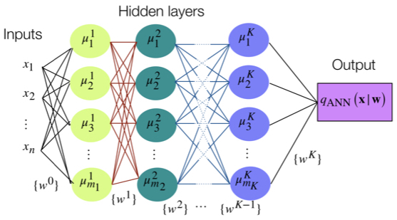
Refer to caption — Figure 1: Schematic representation of the ANN used for deep learning.

We write the unknown reaction coordinate $q\left(\mathbf{x}\right)$ in terms of the following artificial neural network (ANN):

\begin{split}q\left(\mathbf{x}\right)&=q_{\mathrm{ANN}}\left(\mathbf{x}|\mathbf{w}\right)\\ \equiv&\sum_{j_{K}=1}^{m_{K}}h\left(\ldots h\left\{\sum_{j_{2}=1}^{m_{2}}h\left[\sum_{j_{1}=1}^{m_{1}}h\left(\sum_{\alpha=1}^{n}x_{\alpha}w_{\alpha,j_{1}}^{0}+w_{0,j_{1}}^{0}\right)w_{j_{1},j_{2}}^{1}+w_{0,j_{2}}^{1}\right]w_{j_{2},j_{3}}^{2}+w_{0,j_{3}}^{2}\right\}\ldots\right)w_{j_{K}}^{K}+w_{0}^{K},\end{split}

(3)

which represents a network (Figure 1) that takes $x_{1,}x_{2},\ldots,x_{n}$ different inputs, with $K$ hidden layers containing each $m_{1},m_{2},\ldots,m_{K}$ different nodes. The weight matrix $\mathbf{w}$ , i.e., the fitting parameters, defines the connections between nodes, with $w_{ik}^{j}$ connecting node $i$ of layer $j$ with node $k$ of layer $j+1$ . The “activation” function $h$ is a non linear function mimicking the threshold firing behavior of biological neurons.

IV Symbolic Regression

After determining the most relevant inputs we use symbolic regression, and in particular differentiable Cartesian genetic programming, to approximate the trained ANN with a simple expression Izzo et al. 2016. We employ a 1+4 evolutionary strategy for 250 generations where every change in the genome of an offspring is followed by 2500 Newton steps in the weight space of that expression. We add a regularization term $\lambda n$ where $n$ is proportional to the number of active genes to avoid overfitting. We test regularization values of $\lambda\in\left[0.005,0.001,0.01\right]$ .

Table 1: Input relevance analysis for alnine dipeptide. The first 4 most relevant input coordinates and their range of values. All symmetry functions probe the oxygens of water using the parameters in brackets, the subscript to

G

indicates the index of the central atom. Index 5 is the oxygen of the acetyl involved in the peptide bond. Index 12 is the 3 symmetry related hydrogen atom of the methyl-group of alanine and index 16 is the nitrogen of the methylamide.

Index	Definition and range	Normalized relevance $r\left(x_{i}\right)$
$x_{1}$	$\tilde{\psi}=0.5(\cos(\psi+\pi)+1)\in[0.1306,0.9778]$	$1.00$
$x_{2}$	$G^{5}_{5}(\eta=40,r_{s}=0.175,\zeta=64,\lambda=-1)\in[0.0032,1.7550]$	$0.07$
$x_{3}$	$G^{5}_{12}(\eta=40,r_{s}=0.175,\zeta=64,\lambda=-1)\in[0.0035,1.3719]$	$0.05$
$x_{4}$	$G^{5}_{16}(\eta=40,r_{s}=0.175,\zeta=64,\lambda=-1)\in[0.0053,1.5534]$	$0.05$

Table 2: Symbolic regression results for alanine dipeptide. We used as input the first or the four most important coordinates as shown in Table I. Due to the regularization we applied, some input coordinates are not part of the final converged expressions. We used every 10th shooting configurations extracted from the TPS simulation as training set for the symbolic regression. The loss values

L_{\mathrm{ANN}}

and

L_{\mathrm{SR}}

were calculated for the reduced set of points and correspond to the test loss per shooting configuration of the ANN and symbolic regression expression respectively. For every parameter combination the symbolic regression was repeated three times to quantify the stability of the results.

$L_{\mathrm{ANN}}$	Selected coordinates	$\lambda$	$L_{\mathrm{SR}}$	Frequency	Final expression
1.031	1	0.01	1.057	3/3	$\!\begin{aligned} q_{\mathrm{SR}}&=-5.241\tilde{\psi}-1.865\ln(\tilde{\psi})+2.550\end{aligned}$
	1	0.005	1.057	3/3	$\!\begin{aligned} q_{\mathrm{SR}}&=-5.241\tilde{\psi}-1.865\ln(\tilde{\psi})+2.550\end{aligned}$
		0.001	1.057	2/3	$\!\begin{aligned} q_{\mathrm{SR}}&=-5.241\tilde{\psi}-1.865\ln(\tilde{\psi})+2.550\end{aligned}$
		0.001	1.049	1/3	$\!\begin{aligned} q_{\mathrm{SR}}&=-8.377\tilde{\psi}+5.424\end{aligned}$
	4	0.01	1.051	2/3	$\!\begin{aligned} q_{\mathrm{SR}}&=-8.384\tilde{\psi}+5.622\exp(-0.285x_{3})\end{aligned}$
		0.01	1.053	1/3	$\!\begin{aligned} q_{\mathrm{SR}}&=-1.438x_{3}-5.153\ln(\tilde{\psi})-2.172\end{aligned}$
		0.005	1.051	3/3	$\!\begin{aligned} q_{\mathrm{SR}}&=-8.384\tilde{\psi}+5.622\exp(-0.285x_{3})\end{aligned}$
		0.001	1.051	2/3	$\!\begin{aligned} q_{\mathrm{SR}}&=-8.384\tilde{\psi}+5.622\exp(-0.285x_{3})\end{aligned}$
		0.001	1.053	1/3	$\!\begin{aligned} q_{\mathrm{SR}}&=-1.438x_{3}-5.153\ln(\tilde{\psi})-2.172\end{aligned}$

Table 3: Input relevance analysis for LiCl. Range of values of the most relevant coordinates. The symmetry functions are centered on the central atom indicated by the subscript and use the parameters in brackets to probe for the solvent species in square brackets.

Index	Definition and range	Normalized relevance $r\left(x_{i}\right)$
$x_{1}$	$G^{5}_{\mathrm{Li}}(\eta=160,r_{s}=0.7,\zeta=4,\lambda=-1)[\mathrm{Cl}]\in[0.0,0.491]$	$1.00$
$x_{2}$	$G^{5}_{\mathrm{Li}}(\eta=160,r_{s}=0.7,\zeta=64,\lambda=-1)[\mathrm{Cl}]\in[0.0,0.417]$	$0.78$
$x_{3}$	$G^{5}_{\mathrm{Li}}(\eta=160,r_{s}=0.625,\zeta=16,\lambda=-1)[\mathrm{Cl}]\in[0.0,0.007]$	$0.68$
$x_{4}$	$G^{5}_{\mathrm{Li}}(\eta=160,r_{s}=0.625,\zeta=4,\lambda=-1)[\mathrm{Cl}]\in[0.0,0.343]$	$0.45$
$x_{5}$	$G^{5}_{\mathrm{Cl}}(\eta=160,r_{s}=0.7,\zeta=4,\lambda=1)[\mathrm{Li}]\in[0.0,6.940]$	$0.44$
$x_{6}$	$G^{2}_{\mathrm{Cl}}(\eta=300,r_{s}=0.4)[\mathrm{Li}]\in[0.0,5.072]$	$0.38$
$x_{7}$	$G^{5}_{\mathrm{Cl}}(\eta=160,r_{s}=0.7,\zeta=2,\lambda=1)[\mathrm{Li}]\in[0.0,5.678]$	$0.32$
$x_{8}$	$G^{5}_{\mathrm{Cl}}(\eta=160,r_{s}=0.625,\zeta=4,\lambda=-1)[\mathrm{Li}]\in[0.0,\penalty\ 0.971]$	$0.27$
$x_{9}$	$G^{5}_{\mathrm{Li}}(\eta=160,r_{s}=0.175,\zeta=16,\lambda=-1)[\mathrm{O}]\in[0.061,\penalty\ 6.713]$	$0.23$
$x_{10}$	$G^{5}_{\mathrm{Cl}}(\eta=160,r_{s}=0.475,\zeta=4,\lambda=-1)[\mathrm{Li}]\in[0.0,7.666]$	$0.19$
$x_{69}$	$r_{\mathrm{LiCl}}\in[0.240,0.470]$	$0.006$

Table 4: Symbolic regression results for LiCl. We use as input the 3 or 10 most important coordinates and the interionic distance as shown in Table III. Due to the regularization we apply, some input coordinates are not part of the final converged expressions. We used every 10th shooting configurations extracted from the TPS simulation as training set for the symbolic regression. The loss values

L_{\mathrm{ANN}}

and

L_{\mathrm{SR}}

are calculated for the reduced set of points and correspond to the test loss per shooting point of the ANN and symbolic regression expression respectively. For every parameter combination the symbolic regression was repeated three times to quantify the stability of the results.

$L_{\mathrm{ANN}}$	Selected coordinates	$\lambda$	$L_{\mathrm{SR}}$	Frequency	Final expression
0.706	3 + $r_{\mathrm{LiCl}}$	0.01	0.757	3/3	$\!\begin{aligned} q_{\mathrm{SR}}&=29.837r_{\mathrm{LiCl}}-8.485\exp(-0.728x_{1})\end{aligned}$
		0.005	0.757	3/3	$\!\begin{aligned} q_{\mathrm{SR}}&=29.837r_{\mathrm{LiCl}}-8.485\exp(-0.728x_{1})\end{aligned}$
		0.001	0.757	1/3	$\!\begin{aligned} q_{\mathrm{SR}}&=29.837r_{\mathrm{LiCl}}-8.485\exp(-0.728x_{1})\end{aligned}$
			0.754	1/3	$\!\begin{aligned} q_{\mathrm{SR}}&=29.896r_{\mathrm{LiCl}}-8.518\exp(-0.617x_{1})\\ &+4.953x_{2}\end{aligned}$
			0.746	1/3	$\!\begin{aligned} q_{\mathrm{SR}}&=30.115r_{\mathrm{LiCl}}\exp(0.996x_{2})\\ &-8.973\sin(1.260\exp(3.269x_{1}))\end{aligned}$
	10 + $r_{\mathrm{LiCl}}$	0.01	0.753	1/3	$\!\begin{aligned} q_{\mathrm{SR}}&=29.592r_{\mathrm{LiCl}}-8.204\exp(0.028x_{9})\\ &+10.093x_{4}\end{aligned}$
			0.757	1/3	$\!\begin{aligned} q_{\mathrm{SR}}&=29.837r_{\mathrm{LiCl}}-8.405\exp(-0.728x_{1})\end{aligned}$
			0.761	1/3	$\!\begin{aligned} q_{\mathrm{SR}}&=28.993r_{\mathrm{LiCl}}-0.182\ln(x_{9})-8.273\end{aligned}$
		0.005	0.758	2/3	$\!\begin{aligned} q_{\mathrm{SR}}&=29.913r_{\mathrm{LiCl}}-8.473\exp(-1.158x_{4})\end{aligned}$
		0.005	0.757	1/3	$\!\begin{aligned} q_{\mathrm{SR}}&=29.837r_{\mathrm{LiCl}}-8.485\exp(-0.728x_{1})\end{aligned}$
		0.001	0.751	1/3	$\!\begin{aligned} q_{\mathrm{SR}}&=29.510r_{\mathrm{LiCl}}-8.187\exp(-0.866x_{1})\\ &-0.289x_{9}\end{aligned}$
			0.751	1/3	$\!\begin{aligned} q_{\mathrm{SR}}&=29.550r_{\mathrm{LiCl}}-8.214\exp(0.031x_{9})\\ &+6.767x_{1}\end{aligned}$
			0.757	1/3	$\!\begin{aligned} q_{\mathrm{SR}}&=29.837r_{\mathrm{LiCl}}-8.485\exp(-0.728x_{1})\end{aligned}$

References

Jung et al. (2017) H. Jung, K.-i. Okazaki, and G. Hummer, J. Chem. Phys. 147, 152716 (2017).
Izzo et al. (2016) D. Izzo, F. Biscani, and A. Mereta, Lect. Notes Comput. Sci. (including Subser. Lect. Notes Artif. Intell. Lect. Notes Bioinformatics) 10196 LNCS, 35 (2016), arXiv:1611.04766 .