, , , ,
GLISSANDO 3: GLauber Initial-State Simulation AND mOre, ver. 3 Thanks: Supported by Polish National Science Centre, grants 2015/17/B/ST2/00101 (PB), 2015/19/B/ST2/00937 (WB), and 2016/23/B/ST2/00692 (MR)
Abstract
We present ver. 3 of GLISSANDO, a versatile Monte-Carlo generator for Glauber-like models of the initial stages of ultra-relativistic heavy-ion collisions. The present version incorporates the wounded parton model, which is phenomenologically successful in reproducing multiplicities of particle production at the RHIC and the LHC. Within this model, one can study the nucleon substructure fluctuation effects, recently explored in p-A collisions. In addition, the code includes the possibility of investigating collisions of light nuclei, such as 3He and 3H, or the -clustered 7,9Be, 12C, and 16O, where the deformation of the intrinsic wave function influences the transverse shape of the initial state. The current version, being down-compatible, retains the functionality of the previous releases, such as incorporation of various variants of Glauber-like models, a smooth inelasticity profile in the impact parameter obtained from a parametrization of experimental data, fluctuating strength of the entropy deposition, or realistic nuclear distributions of heavy nuclei with deformation. The code can provide output in the format containing the event-by-event source location, which may be further used in modeling the intermediate evolution phase, e.g., with hydrodynamics or transport models. The interface is simplified, such that in the control input file the user may supply only the very basic information, such as the collision energy, the mass numbers of the colliding nuclei, and the model type. GLISSANDO 3 is integrated with the CERN ROOT platform. The package includes numerous illustrative and useful ROOT scripts to compute and plot various results.
Keywords:
ultra-relativistic nuclear collisions, Monte Carlo generators, wounded quarks and nucleons, -clusterization, LHC, RHIC, SPSPROGRAM SUMMARY
Program Title: GLISSANDO 3 ver. 3.42
Licensing provisions: CC By 4.0
Programming language: C++ with the ROOT libraries
Nature of problem: The code implements in a versatile way the
Glauber modeling of the initial stages of ultra-relativistic nuclear collisions, including the wounded nucleon and
wounded quark models, with possible admixture of binary collisions. A state-of-the art inelastic nucleon-nucleon
collision profile is implemented. A statistical distribution of the strength of the sources can be overlaid.
The clustered structure of light nuclei is built in.
Solution method: Monte-Carlo simulation of nuclear collisions, analyzed off-line with numerous ROOT scripts. The software allows for
a straightforward event-by-event analysis of eccentricity coefficients and their correlations, size fluctuations, or multiplicity distributions.
Additional comments including Restrictions and Unusual features: The input may consist only of the model type, the mass numbers of the nuclei and the collision energy.
The output can also be used as initial conditions for further hydrodynamic studies.
1 Introduction
We present an extended version of the package GLISSANDO – GLauber Initial-State Simulation AND mOre, previously described in [1] (ver. 1) and [2] (ver. 2), where the user is directed for a more detailed description of the underlying physics and the features which remain unchanged in the present version.
With the on-going efforts to understand the nature of the ultra-relativistic nuclear collisions, more ideas and models are being explored. Consequently, the dedicated open-access software should follow these efforts and supply useful analysis tools. Concerning the earliest stage of such collisions, modeling based on the so-called Glauber approach [3, 4, 5] has been commonly used, as it works well phenomenologically.
Another dedicated publicly available code implementing the Glauber approach is the PHOBOS Glauber Monte Carlo [6, 7, 8], provided as a ROOT package. The Glauber initial condition is also an option in the parameterizations of TRENTo code [9]. Many other ultra-relativistic nuclear collision codes, e.g., HIJING [10], AMPT [11], URQMD [12], or EPOS [13] use internally the Glauber approach to model the early stage of the collision.
A very successful variant of the Glauber model is based on wounded quarks [14, 15, 16, 17, 18, 19, 20, 21, 22, 23, 24, 25, 26] acting as the particle production sources, rather than the commonly used wounded nucleons [27, 28] amended with binary collisions [29, 30]). Implementation of the wounded quark (or, in general, wounded parton) model is the first major extension in GLISSANDO 3.
Second, collisions of small nuclei with non-uniform distribution of nucleons may offer further stringent tests of the geometry-flow transmutation mechanism, including the event-by-event fluctuations [31, 32, 33, 34, 35, 36, 37, 38, 39, 40, 41, 42, 43, 44, 45, 46, 47, 48, 49, 50, 51, 52, 53, 54, 13, 55, 56, 57, 58, 59, 60, 61, 62, 63, 64, 65]. Moreover, the heavy-light reactions may provide insight into the ground-state clusterization structure in light nuclei, as first proposed in [66, 67] and further explored in [68, 69, 70]. We thus offer a possibility of simulating reactions with 3He (studied experimentally in [71]) or 3H nuclei, which may be thought of as small triangles, as well as collisions involving light -clustered nuclei, such as 7,9Be (dumbbell), 12C (triangle), and 16O (tetrahedron).
The nuclear configurations for 3He and 3H from [72, 73], as supplied with the PHOBOS Glauber Monte Carlo input files [7], are used in GLISSANDO 3 for simulations with nuclei. Similarly, the user has an option to use the configurations for 12C and 16O from [72, 73] as provided in [7].
The user interface to the code has been greatly simplified. In GLISSANDO 3, it suffices to provide the type of the model used (wounded nucleons or wounded partons), the energy of the collision, and the mass numbers of the colliding nuclei. The appropriate inelastic cross section and its profile in the impact parameter are then automatically generated from interpolation formulas based on the experimental scattering data. Specifically, we use here the COMPETE model parametrization implemented in the Particle Data Group review [74], which offers statistically the best description on the and scattering data over a very broad range of the collision energies.
As in the previous releases, the output of GLISSANDO 3 is generated in two ways. The key features of the formed initial states are stored in a ROOT tree containing ready to use results in a compact form. In addition, a full event-by-event output can be generated for use in event-by-event studies of further evolution stages, such as hydrodynamics [35, 75, 76, 77, 59, 78, 79, 80, 81] or transport.
The new features implemented in GLISSANDO 3 include:
- •
State-of-the art nucleon-nucleon inelastic cross sections and their impact-parameter profiles.
- •
Implementation of the wounded quark (in general, wounded parton) model.
- •
Possibility of colliding 3He and 3H, with the distributions from external files.
- •
Inclusion of -clustered structure of 7,9Be, 12C, and 16O nuclei.
- •
Possibility of studying the effect of the proton fluctuations in the framework of the wounded parton model.
- •
Simplified user interface.
The main retained features of the previous releases incorporate:
- •
Parametrization of distributions of all popular nuclei, in particular those used in the energy - system-size scan of the NA61/SHINE [82].
- •
- •
- •
Possibility of studying proton-nucleus and deuteron-nucleus collisions.
- •
Possibility of overlaying weights over the distribution of sources (Poisson, Gamma, negative binomial).
- •
- •
Output of the event-by-event data with location of the sources to a text file, to be used for initialization of hydrodynamics of transport codes.
- •
A reference manual generated with doxygen [92] may be useful for those who wish to tailor the code.
2 New features in GLISSANDO 3
2.1 Inelastic cross sections and inelasticity profiles
With new measurements of the total, elastic, and differential elastic cross section, in particular at the LHC [93, 94, 95] and in cosmic rays [96], new parameterizations of the and scattering amplitudes became available. A standard description is provided by the COMPAS group within the COMPETE model, presented in Sec. 52 of the 2016 edition of the Review of Particle Physics [74], which parametrizes the and scattering data in a very accurate way. In GLISSANDO 3 we use this parameterization of the data as the most complete one.
The inelastic profile function, determining the probability of an inelastic collision at impact parameter and collision energy is defined as
| (1) |
where is the Fourier-Bessel transform of the elastic scattering amplitude ,
| (2) |
with denoting the CM momentum of the nucleon. Using the COMPETE model for with parametrization from [74], we thus obtain . In the code, rather than using these long formulas involving a numerical integration in Eq. (2), we apply a simple parametrization of the inelastic profile of the form [97],
| (3) |
where denotes the incomplete Euler function, is the inelastic cross section, and and are suitably adjusted parameters such that the COMPETE results are accurately reproduced. The values obtained from our fit can be efficiently represented with interpolating functions (which we use for GeV):
| (4) | |||||
Note that the applied expressions are for shear numerical convenience and do not reflect physical mechanisms of high-energy scattering.
The quality of the interpolating formulas is illustrated in Fig. 1, where we compare the inelastic profile functions from the COMPETE model to Eq. (3) with parameters (4) for three selected collision energies. In the left panel of Fig. 2 we show the results of the COMPETE model for the total inelastic cross section (solid line) and our simple fit of Eq. (4). We also show (dotted line) the parametrization , with mb and mb, used in [8]. We note that whereas at higher collision energies ( GeV) this parametrization agrees with the COMPETE model (and thus with the data) accurately, for GeV the COMPETE parametrization, or our Eq. (4), is clearly advantageous. The interpolated dependence of parameters and on the collision energy, as given by formulas (4), is displayed in the right panel Fig. 2.
We recall that the use of a realistic inelasticity profile (as opposed to sometimes used hard-sphere profile in older software, e.g., [10]) is phenomenologically important. First, it leads to proper elastic differential cross section in collisions, as shown above. Second, it yields sizable effects in standard observables in ultra-relativistic nuclear collisions. In particular, the effect on ellipticity of the fireball was discussed in detail in [98], where the use of a realistic (smooth) wounding profile led to a significant (10-20%) reduction for peripheral A-A collisions, compared to the case with a hard-sphere profile.
2.2 Wounded partons
In the wounded quark model [14, 15, 17, 16] the valence quarks play the role of elementary scatterers. The approach is implemented in GLISSANDO 3, as it has proved to be phenomenologically successful in describing the multiplicity of produced hadrons in a variety of reactions, with the linear scaling
| (5) |
well satisfied. Here denotes the observed charged hadrons, and the number of wounded quarks in a given reaction and centrality class. It was first noticed that the RHIC data follow the scaling [18], further explored at RHIC by the PHENIX Collaboration [20, 21], as well as at the SPS [19]. See also [7, 20, 21, 23, 22, 24, 25, 26] for further developments.
Our implementation of the model is described in detail in [23]. The nucleon consists of partons ( for the wounded quark model) distributed according to a radial density
| (6) |
The scale parameter controls the size of the nucleon built of partons. The factor accounts for the center-of-mass corrections; a shift to the center of mass of the nucleon is carried out after randomly generating the positions of the centers of the partons. As is adjusted phenomenologically (see the following), the presence of the factor in formula (6) is conventional.
In the wounded parton approach one needs to choose the parton-parton inelasticity profile. We take it in the Gaussian form
| (7) |
where is the parton-parton inelastic cross section.
Thus our wounded parton model implementation brings in two parameters: and . Their values are chosen in such a way that the resulting collision profile reproduces the COMPETE parametrization discussed in Sec. 2.1. In other words, we impose the desired feature that the inelasticity profile is the same if one uses nucleons or partons as elementary scatterers. With our chosen parameterizations of Eq. (6) and (7) this cannot be accomplished in an exact manner, but optimization leads to a close agreement (within a few percent). This can be seen in Fig. 3, where we compare the elasticity profiles (multiplied with ) obtained in the nucleon and parton models for TeV. The quality of agreement is similar at other collision energies or values of .
The optimum values of the wounded parton model parameters are interpolated as follows for the parton-parton cross section and the parton distribution parameter:
| (8) | |||
| (9) | |||
The above parameterizations work for . The dependence of and on is visualized in Fig. 4. We note that in our model the parton-parton cross section decreases with , whereas the dependence of the size parameter exhibits a rather weak growth with . We also note that an approximate scaling holds, which is accurate to a few percent for .
As in previous releases of our code, centers of nucleons in a nucleus are distributed according to a Woods-Saxon density with additional repulsion [1], or are taken from external calculations, e.g., [86] of [7]. Nuclear shape deformation [99, 83, 84, 100] is implemented for deformed nuclei, such as 63Cu, 197Au, or 238U, in the same manner as in GLISSANDO 2.
2.3 Reactions with light clustered nuclei
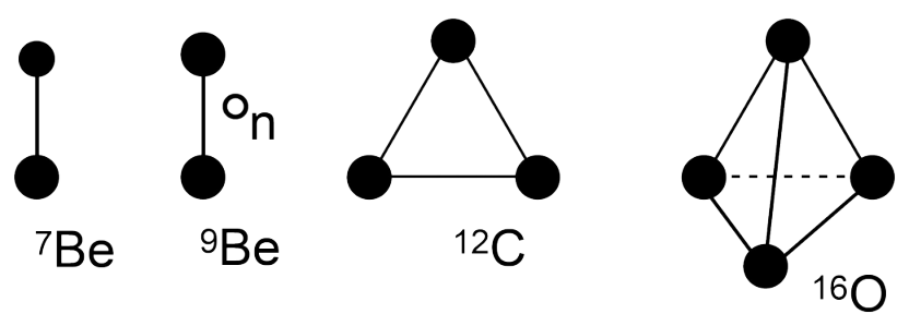
GLISSANDO 3 offers a possibility to collide nuclei whose structure exhibits clustering. Specifically, we implement 7Be as He, 9Be as neutron, 12C as , and 16O as (see Fig. 5). The details of our fixing of geometric parameters of the distributions are presented in [69]. The parameters are adjusted in such way that the one-body nuclear distributions [72, 73] are matched. We first arrange the positions of clusters as in Fig. 5, separating the centers by the distance . The distribution of the centers of nucleons in each cluster is randomly generated according to a Gaussian
| (10) |
where denotes the coordinate of the nucleon and is the position of the center of the cluster . The width of the cluster is controlled with , the rms radius of the cluster. Then the positions of the nucleons are generated sequentially, switching between clusters 1, 2,…, 1, 2,…, until all the needed nucleons are placed.
| Nucleus | [fm] | [fm] | [fm] | [fm] |
|---|---|---|---|---|
| 7Be | 3.2 | 1.2 | 1.4 | - |
| 9Be | 3.6 | 1.1 | - | 1.9 |
| 12C | 2.8 | 1.1 | - | - |
| 16O | 3.2 | 1.1 | - | - |
For the case of 9Be we place the extra neutron on top of the two clusters. The distribution is
| (11) |
and it exhibits a hole in the middle.
The values of parameters used in the code for the cluster model are collected in Table 1.
One may do many physical studies with light clustered nuclei, in particular looking for clusterization signatures in harmonic flow patterns [66, 67, 69, 101]. In Fig. 6 we present an example of a quantity, the symmetric cumulant of elliptic and triangular flows, which displays different behavior on the model with clusters compared to the case without clusters (uniform).
2.4 Smearing of sources
The Monte Carlo Glauber model provides, event-by event, the positions of point-like sources (wounded objects) in the transverse plane. Physically, the sources must have transverse size, which is accomplished by smoothing them, typically with a Gaussian form
| (12) |
where are the transverse coordinates and gives the location of the th source, and is the smearing width. Smearing is necessary, i.a., in forming the initial condition for subsequent hydrodynamic evolution. Moreover, smearing increases the size of the fireball and reduces the eccentricities, which are its basic characteristics. The effect is particularly relevant for small systems. The effects of Gaussian smearing (12) are simple to implement, as the corresponding expressions are analytic.
The eccentricity of rank () in a given event, , and the corresponding angle of the principal axis (the event-plane angle), , are defined in the standard way as
| (13) |
where is the transverse entropy distribution, and we have introduced the polar coordinates via , . When the sources are point-like, then and
| (14) |
where runs over all the sources in the event, and , . With Gaussian smearing (12), we have and, correspondingly,
| (15) | |||
In polar coordinates we may write explicitly
Integration over yields
| (17) |
and integration over
| (18) |
which means that the numerator with smearing in Eq. (2.4) is exactly the same as for point-like sources in Eq. (14).
Repeating the above steps for the denominator yields
| (19) | |||
where is the Euler Gamma function and is the Laguerre polynomial. The forms of for the first few even values of are
| (20) | |||
For odd values of
| (21) | |||
where are the modified Bessel functions of the first kind. It is apparent from the above formulas that smearing increases the denominators, therefore is quenched, in agreement with intuition. At the same time we observe that the principal axes angles are not altered by smearing.
The reduction of the contribution of a single source placed at for first few eccentricities, quantified with , is shown in Fig. 7. We note that, as expected, the effect increases with and with the value of the smearing parameter .
Taking for definiteness the ellipticity and collecting the contributions from all sources, we find the smearing reduction factor , which becomes increasingly important with decreasing mean squared radius, , of the fireball.
Smearing is incorporated in GLISSANDO 3 in the evaluation of eccentricities and the mean squared radius of the fireball. The amount of smearing is controlled with the parameter DS, whereby it has the interpretation of the Gaussian width in one dimension.
2.5 Rapidity modeling
The modeling in rapidity, present to some extent in ver. 2 of the code, has been removed. This is because, unlike the modeling in the transverse plane where the Glauber approach became one of the standards, the longitudinal modeling has much more freedom and is under development. If the user wishes to model the rapidity dependence of the fireball, she/he may use the transverse distributions (generated event-by-event and written to an output file) in an external application.
3 Installation and running
The user must first install the CERN ROOT package [102]. After downloading and unpacking GLISSANDO 3, the command
make
should be run, which creates the executable binary glissando3.
To optionally recreate the doxygen manual (provided as /doc/latex/refman.pdf with the distribution), the doxygen [92] package should be installed and the following commands executed:
make cleandoc
make doc
With the code installed, the user may look at an instructive presentation of the main features of the present version by executing the shell script
./demo_ver_3.sh
To see the created pdf files evince should be installed prior to the run. To use another pdf viewer, the line VIEW=evince should be edited in the *.sh files. The features of ver. 2, retained in the present release, may be explored by executing
./demo_ver_2.sh
For collisions of two nuclei, the standard running command has the syntax
./glissando3 [input_file] [output_file]
where the nuclei can be any, including the proton and the deuteron. When the input or output arguments are absent, the defaults are
input.dat - default input
glissando.root - default output
The input parameters with their defaults are collected in Appendix A.
3.1 Makefile
The Makefile contains commands for compilation and linking. It can be used for profiling the code by modifying the preprocessor options. Most importantly, the user should decide if she/he uses the wounded nucleon or the wounded parton version of the model. In the nucleon case the standard preprocessor options should read
PREPROCESS   := -D_partons_=0 -D_nnwp_=2
  -D_bindep_=1 -D_files_=0 -D_profile_=0 -D_weight_=0 -D_evout_=0
  -D_clusters_=0 -D_uncluster_=0 -D_pardis_=0 -D_rdsconv_=1
whereas for the wounded parton model
PREPROCESS   := -D_partons_=1 -D_nnwp_=1
  -D_bindep_=1 -D_files_=0 -D_profile_=0 -D_weight_=0 -D_evout_=0
  -D_clusters_=0 -D_uncluster_=0 -D_pardis_=0 -D_rdsconv_=1
The meaning of all preprocessor parameters is as follows:
 _nnwp_=0 - hard-sphere NN wounding profile, =1 - Gaussian, =2 - gamma
 _bindep_=1 - binary and wounding depend on each other, =0 - do not
 _files_=1 - read the nuclear distributions from external files,
           =0 - generate randomly
 _profile_=1 - generate the nucleon profile and NN correlation data, =0 - do not
 _weight_=1 - generate data for the NN collision profiles
                      and for the weight (RDS) ditributions, 0 - do not
 _evout_=0 - do not generate the text event data, =1 - short, =2 -long
 _clusters_=1  - generate clusters in light nuclei, =0 do not
 _uncluster_=1 - smoothe out the alpha clusters in nucleus A,
                   =2 - in nucleus B,
                   =3 in both nuclei,
                   =0 - do not smoothe
 _partons_=1 - wounded parton model, =0 - wounded nucleon model
 _pardis_=0  - exponential parton distribution in nucleus, =1 - Gaussian
 _rdsconv_=2 - convention for RDS: 1 - Nw/2, 2 - Nw
The user may modify the Makefile file to suit his needs, or, alternatively, run make for example as follows:
make ’PREPROCESS = -D_partons_=1 -D_nnwp_=1 -D_evout_=1 ’
to produce the binary code for the wounded parton model with the Gaussian wounding profile and with generation of some results to an external ASCII file.
Another functionality is the storage of the current version of the package,
make package
as well as the cleaning options:
make clean
make cleandoc
make cleanoutput
3.2 Input
The input file is a standard ASCII file. Every line contains the name of the parameter separated with space from the assigned value. The sequence of the lines with parameters is flexible. When a parameter is missing in the input file, or a line containing it is commented out with #, the default value is used. See Appendix A for details concerning the input parameters.
3.3 Output
A typical output from a run of GLISSANDO 3 to the console is shown in Table 2.
user@host: ~/GL3$  ./glissando3
Start: Mon Nov 12 15:36:16 2018
--------------------------------------

*********************************************************
GLISSANDO 3 ver. 3.3
ver. 3: http://arxiv.org.abs/1901.04484
ver. 2: Computer Physics Communications 185 (2014) 1759, arXiv:1310.5475
ver. 1: Computer Physics Communications 180 (2009)   69, arXiv:0710.5731
**********************************************************
Simulation of nuclear collisions in Glauber models
----------------------------------------------------------
parameters reset from default in input/input.dat:
EVENTSΨ2000
NUMAΨ208
NUMBΨ208
ECMΨ2760

generates ROOT output file output/glissando.root

number of events: 2000

208+208 @ sqrt(s_NN)=2760GeV

Woods-Saxon: RA=6.40677fm, aA=0.459fm, dA=0.9fm
Woods-Saxon: RB=6.40677fm, aB=0.459fm, dB=0.9fm

NUCLEON MODEL
mixed model: sig_w=61.9917mb, sig_bin=61.9917mb, alpha=0.12
RDS distribution scale with u=1 (wounded) and u=1 (binary)
gamma wounding profile, G=0.972569, omega=0.586854
source smearing width: 0.4 fm
acceptance window: b_min=0fm, b_max=25fm, Nw_min=2, Nw_max=100000

event: 2000     (100%)

Some quantities for the specified acceptance window
(+/- gives the e-by-e standard deviation):
A+B cross section = 7226.7mb  (makes sense for min. bias)
efficiency (accepted/all) = 36.8053%
N_w = 113.994+/-114.84
RDS: 93.5426+/-107.285

Finish: Mon Nov 12 15:37:04 2018
(0h:0m:48s)
**************************************
The results of the simulation are stored in the ROOT output file or, optionally, also in text files when the preprocessor parameter _evout_=1 or 2 is used.
To see the physical results, the user should enter the ROOT environment
root
and execute one of the supplied scripts *.C
.x macro/demo_3/<script name>.C(<optional parameters>)
or directly examine the output ROOT file, e.g. with a
TBrowser a
command (executed within ROOT environment). An alternative method of executing the ROOT scripts is provided in the example shell demo_ver_3.sh. Proceeding this way does not require a greater familiarity with ROOT.
The preprocessor option _evout_ controls the possible event-by-event output to an additional external ASCII file with the name of the ROOT output file appended with .points. If _evout_=2, then the file stores the transverse positions event-by-event. Its content consists of the blocks
RDS NwAB specA atan2(ycmA,xcmA) specB atan2(ycmB,xcmB)
followed with NwAB lines of the format
x y z c w
The second part of the block is
Nbin
followed with Nbin lines of the format
x y z c w
Above we use the notation RDS for the relative deposited strength in the event (defined below), NwAB for the number of wounded objects (nucleons or partons), specA for the number of spectators from nucleus A and atan2(ycmA,xcmA) for the azimuthal angle of their center of mass relative to the axis, and specB and atan2(ycmB,xcmB) for analogous quantities for nucleus B, and Nbin for the number of binary collisions. Next, x and y are the transverse coordinates of the sources in fm, z is the longitudinal coordinate, |c| indicates how many times a wounded nucleon collided, with positive (negative) c corresponding to nucleus A (B), while c=0 indicates the binary collisions. The last entry is the weight w of the given source (by source we customarily mean a wounded nucleon or a binary collision). The number of blocks is equals to the number of events.
If _evout_=1, then a simplified output is generated, with the format
NwA NwB Nbin RDS
where NwA and NwB are the numbers of wounded objects in nuclei A and B, respectively. The number of output lines equals to the number of events.
3.4 Reading external nuclear distributions
The user may provide external files with nuclear distributions. We have used two sets of such files. The first one comes from Alvioli et al. [86] for the case of 16O, 40Ca, and 208Pb. They can be obtained from http://sites.psu.edu/color/. The user must create from the downloaded files a singe file, for instance running
cat ca40-1.dat ca40-2.dat ca40-3.dat [more files] > ca40.dat
The resulting file o16.dat should be placed in the relative subdirectory nucl.
The files have the format
x y z k
where x, y, and z denote the Cartesian coordinates of the centers on nucleons in fm, while for neutrons and for protons. Groups of A lines, where A is the mass number of the nucleus, correspond to a single nuclear configuration.
The second case concerns 3He or 3H distributions, which are taken from the Green’s function Monte Carlo simulations [103] as provided in [7]. For the user’s convenience the files he3_plaintext.dat and h3_plaintext.dat are also provided at the GLISSANDO web site. The format of these files is
x1 y1 z1 x2 y2 z2 x3 y3 z3 foo foo foo foo
where (xi, yi, zi) are the Cartesian coordinates of the th nucleon in a given configuration.
Similarly, the configurations of 12C or 16O from [103] as provided in [7] may be used. They are provided at the GLISSANDO web site as carbon_plaintext.dat and oxygen_plaintext.dat.
To use the nuclear configurations from external files, the code must be compiled with
make ’PREPROCESS = -D_files_=1’
and executed as
./glissando3 [input_file] [output_file] [nucleus_A_file] [nucleus_B_file]
When the syntax
./glissando3 [input_file] [output_file] [nucleus_A_file]
is used, then the distribution of the nucleons in nucleus A is read from an external file, whereas for nucleus B the positions of nucleons are generated randomly. This syntax must also be used for the collisions of nucleus A with the proton or the deuteron.
3.5 Fixing centrality cuts
We explain how to impose centrality cuts on GLISSANDO 3 simulations and how to properly choose the range for the impact parameter (a too large range slows down the simulations). The supplied shell script centrality.sh implements the following procedure. First, a minimum-bias simulation must be run, with no (or broad-range) values for the W0, W1, RDS0, and RDS1 parameters, as well as BMIN=0 and BMAX set to a larger value than the sum of the radii of the two colliding nuclei. We typically use BMAX as about twice this sum to account for the tails in the Woods-Saxon distributions. Note, however, that large values for BMAX lead to a larger Monte Carlo rejection rate,slowing down the simulation. Next, the macro/demo_3/cent.C script should be executed in root. The values of W0, W1, or RDS0, RDS1 corresponding to the desired centrality classes can be read off from the generated file output/centrality.dat. Next, the input file must be modified with the proper values for W0, W1 supplied (if centrality is determined by the multiplicity of the wounded objects), or RDS0, RDS1 (if centrality is given by the relative deposited strength RDS), and the code must be rerun (with low statistics). Running /macro/demo_3/b_dist.C and looking at the plot b_dist.pdf allows us to determine the optimum values for BMIN=0 and BMAX. We thus should update these parameters in the input file and rerun simulations with full statistics.
The above steps can be simply traced by executing centrality.sh.
4 Structure of the code
The structure of the code is provided in the supplied reference manual created with doxygen.
5 Summary
We have presented GLISSANDO 3, with hopes it will continue to be a useful and versatile tool for the heavy-ion community. The authors most welcome suggestions and questions from the users.
We would like to thank dr Maksym Deliyergiyev for his help to make our scripts compatible with ROOT6.
This research was carried out in laboratories created under the project ”Development of research base of specialized laboratories of public universities in Swietokrzyskie region” no POIG 02.2.00-26-023/08 dated May 19, 2009.
Appendix A Input and output
The input parameters are collected in Table 3. The hash sign # at the beginning of the line in the input file comments it out, in which case a default value of the parameter as set in the code (file functions.h) is used.
| name | default | description |
|---|---|---|
| ECM | -1 | center of mass energy of the colliding system [GeV] |
| NUMA | 208 | mass number of nucleus |
| NUMB | 208 | mass number of nucleus |
| EVENTS | 10000 | number of generated events |
| BMIN | 0. | minimum impact parameter [fm] |
| BMAX | 25. | maximum impact parameter [fm] |
| W0 | 2 | minimum allowed number of wounded nucleons |
| W1 | 100000 | maximum allowed number of wounded nucleons |
| RDS0 | 0 | minimum allowed RDS |
| RDS1 | 100000 | maximum allowed RDS |
| MODEL | 0 | 0 - constant superimposed weight, 1 - Poisson, 2 - Gamma, 3 - Negative Binomial |
| Uw | 1. | Poisson, Gamma, or Negative Binomial mean value for wounded objects |
| Ubin | 1. | Poisson, Gamma, or Negative Binomial mean value for binary collisions |
| Vw | 2. | Gamma or Negative Binomial variance for wounded objects |
| Vbin | 2. | Gamma or Negative Binomial variance for binary collisions |
| NCS | 3 | number of partons in the nucleon |
| NBIN | 40 | number of bins for histograms in , , or |
| RWSA | -1 | Woods-Saxon radius for the distribution of centers, nucleus [fm] |
| AWSA | 0.459 | Woods-Saxon width, nucleus [fm] |
| BETA2A | -1 | deformation parameter , nucleus |
| BETA4A | -1 | deformation parameter , nucleus |
| ROTA_THETA | -1 | rotation parameter (angle ), -1 - random rotation, nucleus |
| ROTA_PHI | -1 | rotation parameter (angle ), -1 - random rotation, nucleus |
| RWSB | -1 | Woods-Saxon radius for the distribution of centers, nucleus [fm] |
| AWSB | 0.459 | Woods-Saxon width, nucleus [fm] |
| BETA2B | -1 | deformation parameter , nucleus |
| BETA4B | -1 | deformation parameter , nucleus |
| ROTB_THETA | -1 | rotation parameter (angle ), -1 - random rotation, nucleus |
| ROTB_PHI | -1 | rotation parameter (angle ), -1 - random rotation, nucleus |
| SNN | -1 | NN (parton-parton) “wounding” cross section [mb] |
| SBIN | -1 | NN (parton-parton) binary cross section [mb] |
| ALPHA | 0.12 | mixed model parameter, 0 - wounded, 1 - binary, 0.12 - LHC@2.76 TeV/nucleon |
| CD | 0.9 | closest allowed distance between centers of nucleons [fm] |
| ISEED | 0 | seed for the random number generator, if 0 a random seed is generated |
| BTOT | range parameter for histograms [fm], default= max(RWSA,RWSB)+AWSA+AWSB | |
| SHIFT | 1 | 1 - shift the coordinates of the fireball to the c.m. in the fixed-axes case, 0 - do not shift |
| DW | 0. | dispersion of the location of the source for wounded objectss [fm] |
| DBIN | 0. | dispersion of the location of the source for binary collisions [fm] |
| WFA | 0 | the w parameter of the Fermi distribution, nucleus |
| WFB | 0 | the w parameter of the Fermi distribution, nucleus |
| FBIN | 72 | number of bins for histograms in the azimuthal angle |
| DOBIN | 0 | 1 - compute the binary collisions also for the case ALPHA=0, 0 - do not |
| GA | 1.0 | central value of the Gaussian wounding profile |
| PP | -1 | power of the transverse radius in the Fourier moments |
| RO | 0 | rank of the rotation axes (0 - rotation rank = rank of the Fourier moment) |
| RCHA | 5.66 | harmonic oscillator shell model density mean squared charge radii of nucleus (12C-nucleus) |
| RCHB | 5.66 | harmonic oscillator shell model density mean squared charge radii of nucleus (12C-nucleus) |
| RCHP | 0.7714 | harmonic oscillator shell model density mean squared charge radii of proton |
| OMEGA | -1 | relative variance of cross-section fluctuations for the Gamma wounding profile |
| GAMA | -1 | central value of the Gamma wounding profile |
| SCALEA | 1. | scale parameter for the size of the nucleus (cluster version) [fm] |
| SIGMAA | 1. | standard deviation of x, y, z coordinates of nucleons in the alpha cluster [fm] |
| SIGMABISA | 1. | standard deviation of x, y, z coordinates of nucleons in the 3He cluster or nucleon no. 9 [fm] |
| SCALEB | 1. | scale parameter for the size of the nucleus (cluster version) [fm] |
| SIGMAB | 1. | standard deviation of x, y, z coordinates of nucleons in the alpha cluster [fm] |
| SIGMABISB | 1. | standard deviation of x, y, z coordinates of nucleons in the 3He cluster or nucleon no. 9 [fm] |
| QSCALE | -1 | scale parameter in the parton distribution function [fm] |
| DS | -1 | source smearing parameter |
References
- [1] W. Broniowski, M. Rybczyński and P. Bożek, Comput. Phys. Commun. 180 (2009) 69, 0710.5731.
- [2] M. Rybczyński et al., Comput. Phys. Commun. 185 (2014) 1759, 1310.5475.
- [3] R. Glauber, High energy collision theory, volume 1 in Lectures in theoretical physics (Interscience, NewYork, 1959).
- [4] W. Czyż and L.C. Maximon, Annals Phys. 52 (1969) 59.
- [5] M.L. Miller et al., Ann. Rev. Nucl. Part. Sci. 57 (2007) 205, nucl-ex/0701025.
- [6] B. Alver et al., (2008), 0805.4411.
- [7] C. Loizides, J. Nagle and P. Steinberg, SoftwareX 1-2 (2015) 13, 1408.2549.
- [8] C. Loizides, J. Kamin and D. d’Enterria, Phys. Rev. C97 (2018) 054910, 1710.07098, [erratum: Phys. Rev.C99,no.1,019901(2019)].
- [9] J.S. Moreland, J.E. Bernhard and S.A. Bass, Phys. Rev. C92 (2015) 011901, 1412.4708.
- [10] X.N. Wang and M. Gyulassy, Phys. Rev. D44 (1991) 3501.
- [11] Z.W. Lin et al., Phys. Rev. C72 (2005) 064901, nucl-th/0411110.
- [12] S.A. Bass et al., Prog. Part. Nucl. Phys. 41 (1998) 255, nucl-th/9803035.
- [13] K. Werner et al., Phys. Rev. C82 (2010) 044904, 1004.0805.
- [14] A. Białas, W. Czyż and W. Furmański, Acta Phys. Polon. B8 (1977) 585.
- [15] A. Białas et al., Acta Phys. Polon. B8 (1977) 855.
- [16] V.V. Anisovich, Yu.M. Shabelski and V.M. Shekhter, Nucl. Phys. B133 (1978) 477.
- [17] A. Białas and W. Czyż, Acta Phys. Polon. B10 (1979) 831.
- [18] S. Eremin and S. Voloshin, Phys. Rev. C67 (2003) 064905, nucl-th/0302071.
- [19] P. Kumar Netrakanti and B. Mohanty, Phys. Rev. C70 (2004) 027901, nucl-ex/0401036.
- [20] PHENIX, S.S. Adler et al., Phys. Rev. C89 (2014) 044905, 1312.6676.
- [21] PHENIX, A. Adare et al., Phys. Rev. C93 (2016) 024901, 1509.06727.
- [22] R.A. Lacey et al., Universe 4 (2018) 22, 1601.06001.
- [23] P. Bożek, W. Broniowski and M. Rybczyński, Phys. Rev. C94 (2016) 014902, 1604.07697.
- [24] L. Zheng and Z. Yin, Eur. Phys. J. A52 (2016) 45, 1603.02515.
- [25] J.T. Mitchell et al., Phys. Rev. C93 (2016) 054910, 1603.08836.
- [26] C. Loizides, Phys. Rev. C94 (2016) 024914, 1603.07375.
- [27] A. Białas, M. Błeszyński and W. Czyż, Nucl. Phys. B111 (1976) 461.
- [28] A. Białas, J. Phys. G35 (2008) 044053.
- [29] D. Kharzeev and M. Nardi, Phys. Lett. B507 (2001) 121, nucl-th/0012025.
- [30] PHOBOS, B.B. Back et al., Phys. Rev. C65 (2002) 031901, nucl-ex/0105011.
- [31] J.Y. Ollitrault, Phys. Rev. D46 (1992) 229.
- [32] C.E. Aguiar et al., Nucl. Phys. A698 (2002) 639, hep-ph/0106266.
- [33] M. Miller and R. Snellings, (2003), nucl-ex/0312008.
- [34] PHOBOS, S. Manly et al., Nucl. Phys. A774 (2006) 523, nucl-ex/0510031.
- [35] R. Andrade et al., Phys. Rev. Lett. 97 (2006) 202302, nucl-th/0608067.
- [36] S.A. Voloshin, (2006), nucl-th/0606022.
- [37] PHOBOS Collaboration, B. Alver et al., Phys. Rev. Lett. 98 (2007) 242302, nucl-ex/0610037.
- [38] H.J. Drescher and Y. Nara, Phys. Rev. C75 (2007) 034905, nucl-th/0611017.
- [39] W. Broniowski, P. Bożek and M. Rybczyński, Phys. Rev. C76 (2007) 054905, 0706.4266.
- [40] S.A. Voloshin et al., Phys. Lett. B659 (2008) 537, 0708.0800.
- [41] R.P.G. Andrade et al., Acta Phys. Polon. B40 (2009) 993, 0812.4143.
- [42] PHOBOS, B. Alver et al., Phys. Rev. C77 (2008) 014906, 0711.3724.
- [43] W. Broniowski, M. Chojnacki and L. Obara, Phys. Rev. C80 (2009) 051902, 0907.3216.
- [44] R. Andrade et al., J.Phys. G37 (2010) 094043, 0912.0703.
- [45] Y. Hama et al., Acta Phys. Polon. B40 (2009) 931, 0901.2849.
- [46] T. Hirano and Y. Nara, Phys.Rev. C79 (2009) 064904, 0904.4080.
- [47] B. Alver and G. Roland, Phys. Rev. C81 (2010) 054905, 1003.0194.
- [48] B.H. Alver et al., Phys. Rev. C82 (2010) 034913, 1007.5469.
- [49] P. Staig and E. Shuryak, Phys.Rev. C84 (2011) 034908, 1008.3139.
- [50] D. Teaney and L. Yan, Phys. Rev. C83 (2011) 064904, 1010.1876.
- [51] G.Y. Qin et al., Phys.Rev. C82 (2010) 064903, 1009.1847.
- [52] J.L. Nagle and M.P. McCumber, Phys.Rev. C83 (2011) 044908, 1011.1853.
- [53] J. Xu and C.M. Ko, Phys.Rev. C83 (2011) 021903, 1011.3750.
- [54] R.A. Lacey et al., Phys.Rev. C84 (2011) 027901, 1011.3535.
- [55] PHENIX Collaboration, A. Adare et al., Phys. Rev. Lett. 105 (2010) 062301, 1003.5586.
- [56] G.Y. Qin and B. Muller, Phys.Rev. C85 (2012) 061901, 1109.5961.
- [57] R.S. Bhalerao, M. Luzum and J.Y. Ollitrault, Phys. Rev. C84 (2011) 054901, 1107.5485.
- [58] R.S. Bhalerao, M. Luzum and J.Y. Ollitrault, Phys. Rev. C84 (2011) 034910, 1104.4740.
- [59] F.G. Gardim et al., Phys. Rev. C85 (2012) 024908, 1111.6538.
- [60] Z. Qiu, C. Shen and U. Heinz, Phys. Lett. B707 (2012) 151, 1110.3033.
- [61] Z. Qiu and U.W. Heinz, Phys.Rev. C84 (2011) 024911, 1104.0650.
- [62] J. Xu and C.M. Ko, Phys.Rev. C84 (2011) 044907, 1108.0717.
- [63] D. Teaney and L. Yan, Phys. Rev. C86 (2012) 044908, 1206.1905.
- [64] J. Jia and S. Mohapatra, (2012), 1203.5095.
- [65] T. Hirano et al., Prog. Part. Nucl. Phys. 70 (2013) 108, 1204.5814.
- [66] W. Broniowski and E.R. Arriola, Phys. Rev. Lett. 112 (2014) 112501, 1312.0289.
- [67] P. Bożek et al., Phys.Rev. C90 (2014) 064902, 1410.7434.
- [68] S. Zhang et al., Phys. Rev. C95 (2017) 064904, 1702.02507.
- [69] M. Rybczyński, M. Piotrowska and W. Broniowski, Phys. Rev. C97 (2018) 034912, 1711.00438.
- [70] S.H. Lim et al., Phys. Rev. C99 (2019) 044904, 1812.08096.
- [71] PHENIX, A. Adare et al., (2015), 1507.06273.
- [72] R.B. Wiringa et al., Phys. Rev. C89 (2014) 024305, 1309.3794.
- [73] D. Lonardoni et al., Phys. Rev. C96 (2017) 024326, 1705.04337.
- [74] Particle Data Group, C. Patrignani et al., Chin. Phys. C40 (2016) 100001.
- [75] K. Werner et al., J. Phys. G36 (2009) 064030, 0907.5529.
- [76] H. Petersen et al., Phys. Rev. C82 (2010) 041901, 1008.0625.
- [77] H. Holopainen, H. Niemi and K.J. Eskola, Phys. Rev. C83 (2011) 034901, 1007.0368.
- [78] P. Bożek, Phys. Rev. C85 (2012) 014911, 1112.0915.
- [79] B. Schenke, S. Jeon and C. Gale, Phys. Rev. Lett. 106 (2011) 042301, 1009.3244.
- [80] Z. Qiu and U.W. Heinz, AIP Conf.Proc. 1441 (2012) 774, 1108.1714.
- [81] A. Chaudhuri, Phys. Lett. B713 (2012) 91, 1112.1166.
- [82] https://na61.web.cern.ch/na61/xc/index.html, NA61/SHINE-Collaboration.
- [83] P. Filip, Phys. Atom. Nucl. 71 (2008) 1609, 0712.0088.
- [84] P. Filip et al., Phys. Rev. C80 (2009) 054903.
- [85] P. Filip, Nucl. Phys. Proc. Suppl. 198 (2010) 46.
- [86] M. Alvioli, H.J. Drescher and M. Strikman, Phys. Lett. B680 (2009) 225, 0905.2670.
- [87] W. Broniowski and M. Rybczyński, Phys. Rev. C81 (2010) 064909, 1003.1088.
- [88] C. Hohne, F. Puhlhofer and R. Stock, Phys. Lett. B640 (2006) 96, hep-ph/0507276.
- [89] F. Becattini and J. Manninen, Phys. Lett. B673 (2009) 19, 0811.3766.
- [90] P. Bożek, Acta Phys. Polon. B36 (2005) 3071, nucl-th/0506037.
- [91] K. Werner, Phys. Rev. Lett. 98 (2007) 152301, 0704.1270.
- [92] http://www.stack.nl/~dimitri/doxygen/.
- [93] TOTEM, G. Antchev et al., Phys. Rev. Lett. 111 (2013) 012001.
- [94] TOTEM, G. Antchev et al., Nucl. Phys. B899 (2015) 527, 1503.08111.
- [95] ATLAS, G. Aad et al., Nucl. Phys. B889 (2014) 486, 1408.5778.
- [96] Pierre Auger, P. Abreu et al., Phys. Rev. Lett. 109 (2012) 062002, 1208.1520.
- [97] M. Rybczyński and Z. Włodarczyk, J.Phys. G41 (2013) 015106, 1307.0636.
- [98] M. Rybczynski and W. Broniowski, Phys. Rev. C84 (2011) 064913, 1110.2609.
- [99] U.W. Heinz and A. Kuhlman, Phys. Rev. Lett. 94 (2005) 132301, nucl-th/0411054.
- [100] M. Rybczyński, W. Broniowski and G. Stefanek, Phys. Rev. C87 (2013) 044908, 1211.2537.
- [101] S. Zhang et al., Eur. Phys. J. A54 (2018) 161, 1808.10265.
- [102] https://root.cern.ch/.
- [103] J. Carlson and R. Schiavilla, Rev. Mod. Phys. 70 (1998) 743.