Practical issues of twin-field quantum key distribution
Abstract
Twin-Field Quantum Key Distribution(TF-QKD) protocol and its variants, such as Phase-Matching QKD(PM-QKD), sending or not QKD(SNS-QKD) and No Phase Post-Selection TF-QKD(NPP-TFQKD), are very promising for long-distance applications. However, there are still some gaps between theory and practice in these protocols. Concretely, a finite-key size analysis is still missing, and the intensity fluctuations are not taken into account. To address the finite-key size effect, we first give the key rate of NPP-TFQKD against collective attack in finite-key size region and then prove it can be against coherent attack. To deal with the intensity fluctuations, we present an analytical formula of 4-intensity decoy state NPP-TFQKD and a practical intensity fluctuation model. Finally, through detailed simulations, we show NPP-TFQKD can still keep its superiority of high key rate and long achievable distance.
I Introduction
Quantum Key Distribution(QKD)Bennett and Brassard 2014; Ekert 1991 is one of the most mature applications among the emerging quantum technologies. It allows two remote users, called Alice and Bob, to share random secret keys even if there is an eavesdropper, EveMayers 2001; Lo and Chau 1999; Shor and Preskill 2000. Due to the loss of channel, both the key rate and achievable distance of QKD are limited. Although increasing the secret key rate(SKR) and achievable distance are essentially significant for the real applications of QKD, the theorists proved there are some limits on the improvement of SKRTakeoka et al. 2014; Pirandola et al. 2017. In particular, for the channel of transmittance , the linear bound Pirandola et al. 2017, i.e. , gives the precise SKR bound for any point-to-point QKD without quantum repeaters. Surprisingly, a revolutionary protocol called Twin-Field Quantum Key Distribution(TF-QKD)Lucamarini et al. 2018 was recently proposed to beat this bound. Inspired by the novel idea of TF-QKD, researchers proposed some variants and completed the corresponding security proofs Tamaki et al. 2018; Ma et al. 2018; Wang et al. 2018; Cui et al. 2019; Curty et al. 2018; Lin and Lütkenhaus 2018. From the view of experiments, these variants, i.e. Phase-Matching QKD(PM-QKD)Ma et al. 2018, sending or not QKD(SNS-QKD)Wang et al. 2018 and No Phase Post-Selection TF-QKD(NPP-TFQKD)Cui et al. 2019; Curty et al. 2018; Lin and Lütkenhaus 2018, are simpler. Indeed, both the SNS-QKD and NPP-TFQKD have been scuccessfully demonstratedMinder et al. 2019; Wang et al. 2019; Liu et al. 2019; Zhong et al. 2019.
However, there are still some gaps between theory and implementation of TF-QKD. The first problem is the finite-key size effect is still not considered previously. In Refs.Cui et al. 2019; Curty et al. 2018; Lin and Lütkenhaus 2018, asymptotic SKR of NPP-TFQKD is proposed, but the SKR in finite-key region is not given. On the other hand, the key-size in a practical implementation is always finite, thus a framework to deal with the finite-key size effect in TF-QKD is indispensable.
Another problem we will discuss is a potential security loophole of TF-QKD and its variants. Although the Refs.Lucamarini et al. 2018; Tamaki et al. 2018; Ma et al. 2018; Wang et al. 2018; Cui et al. 2019; Curty et al. 2018; Lin and Lütkenhaus 2018 have proved the TF-QKD and its variants are information-theoretically secure even with unstrusted measurement device just like the original measurement-device-independent protocolLo et al. 2012; Wang et al. 2015; Liu et al. 2013; Ma and Razavi 2012, the imperfections of laser source may spoil the security. One of the intractable loopholes of source is the intensity fluctionWang et al. 2009; Wang 2007; Zhou et al. 2017. In the existing security proofs of NPP-TFQKD, it is assumed that Alice and Bob are able to accurately control the intensity of signal and decoy modes, which is not perfectly satisfied in experiment. In this work, we also propose a countermeasure to tackle the internsity fluctuation of NPP-TFQKD. A key step of our method is proposing the analytical formulas to deal with the 4-intensity decoy states in NPP-TFQKD. In the original NPP-TFQKDCui et al. 2019, one must use linear programing to solve linear equations of decoy states Lo et al. 2005; Wang 2005a; Wang 2005b; Wang 2013; Yu et al. 2015. Compared with linear programing, analytical formula has superiorities on some special situations. More importantly, the proposed analytical formulas are particularly convinient to be incorporated to our intensity fluctuation. Another key step of our method is introducing a new intensity fluctuation model in finite-key size regime. The model makes TF-QKD robuster to intensity fluctuation.
The rest of this paper is organized as followoing. Firstly, In Sec.II, we briefly review the flow of NPP-TFQKD protocol. In Sec.III, we analyze the finite-key size effect of NPP-TFQKD, give the SKR formula against coherent attack and evaluate the performance of TF-QKD in finite-key regime. In Sec.IV, the analytical formulas for 4-intensity decoy state method are given. Then we introduce the intensity fluctuation model and its countermeasure. Finally, a completed simulation taken both the finite-key size effect and intensity fluctuation into account is present.
II Protocol definition
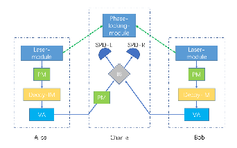
The setup of NPP-TFQKDCui et al. 2019 protocol is illustrated in Fig.1 and the flow is as following:
State preparation: This step will be repeated by trials. In each trial, Alice(Bob) chooses code mode or decoy mode with probabilities and respectively, sends corresponding quantum state to untrusted Charlie.
When code mode is selected, Alice(Bob) prepares a phase-locked weak coherent pulse(WCP) (), where the plus or minus of the quantum state depends on the bit value of Alice(Bob)’s random key of this trial.
When decoy mode is selected, Alice(Bob) prepares a phase randomized WCP, whose intensity () is randomly choosen from a pre-decided set. Alice(Bob) actually prepares a mixed state since the randomized phase in the decay mode will never be publicly announced. For instance, the density matrix of Alice’s WCP in decoy mode can be denoted as:
| (1) |
where is the Fock state.
Measurement: For each trail of the state preparation step, the untrusted Charlie must publicly announce a single click of his single photon detector(SPD) ’SPD-L’ or ’SPD-R’ or non-click meassage. Note that Charlie is untrusted, thus he is not necessarily to make the measurement shown in Fig.1.
Sifting: Alice and Bob publicly announce which trails are code mode and which are decoy mode. For the trials they both choose code mode and Charlie announce ’SPD-L’ or ’SPD-R’ clicked, Alice and Bob will retain this key bit. According to Charlie’s measurement result, Bob may decide to flip his key bit or not. After this step, Alice and Bob generate sifted key bit string and respectively.
Error correction: Alice sends bits of classical error correction data to Bob. Here =|Z|= |Z’| is the size of sifted key bits, is the Shannon entropy, is the error rate of sifted key bits and denotes error correction efficiency. Depending on the error correction data and , Bob obtains an estimated of . Next, by applying universal2 hash fuction, Alice sends bits of error verification information to Bob. If the error verification fails, they output an empty string and abort the protocol. Otherwise, they assume the error correction sucesses and .
Parameter estimation and privacy amplification: Alice and Bob accumulate data to estimate gain of trials that they both choose code mode, gains of trials they choose decoy mode with intensity and respectively. With these parameters and , , Alice and Bob perform privacy amplification, say, apply a random universal2 hash function to and respectively to generate -length secure bit string and respectively. The SKR per pulse is defined as
III finite-key analysis of NPP-TFQKD
Previous worksCui et al. 2019; Curty et al. 2018; Lin and Lütkenhaus 2018 of NPP-TFQKD are based on the asymptotic situation. However, since it’s impossible for Alice and Bob to send infinite pulses to generate their secure key in reality, the finite-key size effectChristandl et al. 2009; Sheridan et al. 2010; Ma et al. 2012; Curty et al. 2014 must be taken into account. In this section, we first extend the asymptoic SKR formula of Ref.Cui et al. 2019 to non-asymptotic one against collective attack. Then based on the postselection technique developed in Ref.Christandl et al. 2009, a formula against coherent attack is present.
III.1 Security definition and SKR against collective attack
As discussed above, in the end of NPP-TFQKD, Alice and Bob obtain a pair of bit string and respectively. Ideally, the bit strings are secure and applicable to any cryptosystem if two fundamental conditions are met, namely correctness and secrecy. The correctness is, in simple terms, , which is guarantted by the error verification. The secrecy requires Eve’s system is decoupled from Alice’s key , which is illustrated by , where denotes the density matrix of Alice and Eve’s quantum state, denotes the uniform mixture of all possible value of , denotes the orthonormal basis of Alice’s key and is Eve’s the density matrix of Eve’s system conditioned that Alice’s key is in the state . Clearly, Alice’s key is completely unknown to Eve in this ideal case.
However, in finite-key size regime, the ideal condition usually can’t be perfectly met. In Ref.Müller-Quade and Renner 2009, a composoble secruity criteria is proposed. This criteria introduces secure parameters to describe some small probabilities of the keys and varing from the ideal case. The protocol is -correct if , i.e. the probability of is less than . Similarly, the protocol is -secret if , which means is close to the ideal situation , where the symbol denotes trace norm of matrix . In general, if a protocol is -secure, must hold. To meet this criteria, with the same manner of Ref.Sheridan et al. 2010, the SKR formula of NPP-TFQKD against collective is given by
| (2) |
where is the size of sifted key bits, is the upperbound of Eve’s information on the sifted key bit if she launches collective attack, implies that , accounts for the probability of failure of privacy amplification, and measures the accuracy of the estimating the smooth min-entropySheridan et al. 2010. As shown in Ref.Cui et al. 2019, the estimation of against collectice attack depends on some experimentally observed parameters including the gains and . When the number of trials is finite, the expectations of these gains may vary from the experimentally observed values due to statistical fluctuations. Thus, another secure parameter Curty et al. 2014 characterizing the probablilty that parameter estimation fails must be taken into account. For instance, consider a set of random variables , the observed frequency of bit is usually not equal to its expectation , provided is finite. To solve this problem, we apply large deviation theory, specifically, the Chernoff bound to estimate a confidence interval of according to the obeserved value. In NPP-TFQKD, we can apply Chernoff boundCurty et al. 2014; Wang et al. 2017; Tang et al. 2014 to estimate and through the observed gains and with a failure probability respectively. For instance, we have that the expectation value of the gain satisfied with probability , where
| (3) | ||||
, , and denotes the total number of trails which Alice and Bob select decoy mode with intensity and , respectively. As there are totally 11 gains to estimate in NPP-TFQKD Cui et al. 2019, the probability of occuring any failure in the estimations of 11 gains is . Then applying the worst-case fluctuation analysis in the calculation of linear programmingWang et al. 2017; Yu et al. 2015, we can bound , where is the probability of Charlie announcing a click message conditioned that Alice and Bob send Fock states and respectively. Furthermore, with Eq.(2) in Ref.Cui et al. 2019, we obtain with the failure probability of .
Finally, Alice and Bob generate bits secret key against collective attack with -security. Obviousely, is not exceeding the sum of failure probabilities of error verification, privacy amplification, accuracy of smooth min-entropy and parameters estimation, say,
| (4) |
Now we have introduced how to generate -security keys against collective attack in NPP-TFQKD with finite-key effect. Next, we discuss how to obtain -security keys against coherent attack.
III.2 Countermeasure of coherent attack
According to Ref.Christandl et al. 2009, it is proved that for a QKD protocol, the security against collective attack could be extended to be against coherent attack easily. We introduce the following corollary from the theorem 1 of Ref.Christandl et al. 2009 to tackle coherent attack in finite-key region.
. The key rate against coherent attack could be given by
| (5) |
while the key is -secure and
| (6) |
. The proof is based on the theorem 1 of Ref.Christandl et al. 2009 and very similar proofs can be found in Ref.Christandl et al. 2009 and the appendix B of Ref.Sheridan et al. 2010. We denote , , and are the Hilbert space of Alice’s ancilla , Bob’s ancilla and Clarlie’s message respectively. Without compriomising the security, Charlie’s messgage (click or not) can be treated as a quantum stated shared by Alice and Bob. The NPP-TFQKD protocol using Eq.2 to generate keys could be viewed as a map tranforming , and into keys and () respectively. Let be a hypothecal map tranforming imperfect keys and into perfect ones and define . Recall last subsection, it asserts that holds when Eq.2 is used to generate keys, where the de Finetti-Hilbert-Schmidt state , , is the pure state shared by Alice, Bob and Eve induced by any collective attack, and is the Haar measure on the pure state .
Next, we consider Eve may control another ancilla to obtain the purification of . For such a purification, is not larger than Christandl et al. 2009 where . Through controlling ancilla , Eve’s min-entropy on sifted key is decreased at most bits. To meet the security, Alice and Bob may perform protocol , in which privacy amplification shortens the sifted key into bits. Then we have still holds, where is a hypothecal map generating perfect keys.
Finally, we apply the theorem 1 of Ref.Christandl et al. 2009 and obtain
Since is any state shared by Alice, Bob and Eve, this inequality clearly shows that the protocol is -secure for any coherent attack. Substituting , we end the proof.
According to the corollary, if Alice and Bob want to generate -secure keys against any attack, they will calculate the parameter with Eq.6, and generate keys with the fromulae Eqs.5, 2 and 4.
To evaluate the performance of NPP-TFQKD in finite-key region, simulations in fiber channel are performed here. We assume the dark-count rate of SPD is per trial, the detection efficiency is and optical misalignment is . The attenuation of fiber is and the fiber tranmittance is where is fiber length. The total secure parameter in Eq.6 is fixed as . In addition to fixed parameters above, there are some parameters should be optimized to maximize the SKR. There are 10 parameters should be optimized in total. The first set is decoy intensities , and . The second set is probabilities of modes and intensities. denote probabilities of choosing code mode and denote probabilities of choosing decoy mode with intensity , , . It worth noting that probabilities of vacuum state is . The number of pulses they both select code mode is and they select decoy mode with intensity and respectively is . The other set is , , and satisfying Eq.4. Define , , and .
The optimized paramters can be regarded as a vector . Noting that the convex form of function Lu et al. 2019; Wang and Lo 2018 is not guaranteed, we choose particle swarm optimization algorithm(PSO) which can optimize the non-smooth function and non-convex functionKennedy 2010 to search the best to maximize the .
The results of the simulations are illustrated in Fig.2 and 3. In Fig.2, we fix the pulses number to be , , and simulate the SKR as a function of distance between Alice and Bon. In Fig.3 the distance is fixed to be , and , then we simulate the SKR as a function of . The results show that compared with asymptotic situation, the protocol still works well in non-asymptotic situations and the linear bound is still overcomed when .


IV NPP-TFQKD with both large random intensity fluctuation and finite-key size effect
Except for finite-key size effect, a ubiquitous loophole in practical QKD system is intensity fluctuationZhou et al. 2017; Wang et al. 2009; Wang 2007. When applying decoy state technique, accurate intensity values are required to ensure the correct estimation of Cui et al. 2019. However, it’s very difficult to control the intensity of WCP exactly in practical QKD system since noise, time jitter, problem of modulation and other imperfections of devices. It brings potential loopholes and may allow Eve to perform sophisticated attacks. In this section, we discuss the NPP-TFQKD with large random intensity fluctuation in finite-key size regime. The main contribution of this section is that we present a countermeasure of both large random intensity fluctuation and finite-key size effect of NPP-TFQKD. By applying our method, the NPP-TFQKD with large random intensity fluctuation can remain its advantage of breaking the linear bound.
IV.1 Analytical formula of 4-intensity decoy state method of NPP-TFQKD
Before proposing the intensity fluctuation model of NPP-TFQKD, we will introduce our analytical formula of 4-intensity decoy state method. In ’Parameter estimation and privacy amplification’ step, the n-photon yield can be estimated by linear programming or analytical formulaWang 2013; Yu et al. 2015. However, the analytical formula of NPP-TFQKD is not given. In our countermeasure of imperfect WCP source loophole in next section, the analytical formula is needed. To make the NPP-TFQKD more practical, the analytical formula of 4-intensity decoy state method is proposed.
Define where . To estimate the upper bound of , we have to estimate the upper bound of , , , , , and lower bound of . The upper and lower bound of can be estimated by applying linear programming whose constraints are joint of:
| (7) |
where . Noting that these depend on the intensity , it’s obvious that the in Eq.(7) are uncertain and the linear programming will be not valid any more if we can’t control intensities exactly. Intuitively, we can still get secure bound of key rate if we correctly replace coefficients by its upper and lower bound in analytical formula. Thus we present an analytical formula before building the fluctuation model.
We will use superscript or subscript and to express, respectively, upper and lower bound of a variable and we denote intensities in decoy mode by ,, , where and is the vacuum state. It is worth noting that, the intensity of code mode should be the same as one of , or . To make our formula more clear, we suppose code mode intensity is and denote by , , .
Here we will demonstrate how to estimate n-photon yield by analytical formulas as follows. The details are showed in Appendix.
Estimation of :
.
Upper bound of and :
| (8) |
where , and .
Expression of is similar, the difference is , , .
Upper bound of and :
| (9) |
where , . Formula of is similar but , .
Upper bound of :
| (10) |
Lower bound of :
We take two steps to calculate the . Define , where and .
| (11) | ||||
where and
The lower bound of is
| (12) |
IV.2 Estimation of average intensity
In this subsection, we briefly introduce the simple tomography technique proposed by Ref.Wang 2007. Based on this work, we propose a large random intensity fluctuation model in finite-key size regime.
As illustrated in Fig.4, Alice (Bob) should firstly produce a WCP with intensity when she(he) actually wants . Before sending the WCP to Charlie, she (he) splits it by a 50:50 BS. One of the pulse is sent to Charlie and the other one is measured by a local low dark-count SPD whose detection efficiency is . After sending -intensity WCPs, the local detector’s count number is where the dark count is ignored since it’s orders of magnitude lower than light count. Because of the random fluctuations, whenever Alice (Bob) wants to modulate intensity , she (he) actually modulates , where is the average intensity and the instantaneous fluctuation is an unknow value. Mathematically, the click rate is:
| (13) |
However, this conclusion in Ref.Wang 2007 can’t be used in non-asymptotic situations directly. Here we apply large deviation theory to make the method met practice.
Noting that the distribution of intensity fluctuation is not independent identically distributed in most cases, we choose Azuma’s inequalityYin et al. 2010; Boileau et al. 2005; Azuma 1967 rather than Chernoff bound to estimate the confidence interval of . When the observed count number is , The upper and lower bound of is:
| (15) | ||||
where the is secure parameter of estimation. Then the bound of the average intensity is corrected as
| (16) | ||||

IV.3 Model of NPP-TFQKD with both intensity fluctuation and finite-key size effect
In this subsection, we will propose our countermeasure model. Firstly, we should define some symbols. Let’s take the first decoy state(intensity is ) as an example. When we want sent -intensity weak coherent pulse, we actually prepare since the intensity fluctuation. The intensity range is where and .
With definitions above, the density matrix of the source with fluctuation can be describe by:
| (17) |
and the is re-written as:
| (18) |
By applying taylor expansion to Eq.(18), we get:
| (19) | ||||
Noting an important fact that , we find the first order item of is not exist in Eq.(19). i.e, the Eq.(19) can be re-written as:
| (20) |
Define function , . and are, respectively, maximum and minimum values which can be easily found by optimization algorithms in interval . and are, respectively, maximum and minimum value points.
Noting that the function is monotonically increasing function when and , when , we can obtain a tight bound of as
| (21) | ||||
Espacially, when ,
| (22) |
However, without introduction of average intensity, when :
| (23) |
and when :
| (24) |
The difference between introducing average intensity or not is showed in Fig.5, it indicates that the introduction of average intensity can significantly tighten the bound.
By substituting Eq.(3),(21) and (22) into our analytical formula, we can obtain bounds of in uncertain intensity and finite-key size regime.
Upper bound of :
;
Upper bound of and :
We take as example, the is similar.
| (25) |
where , and .
Upper bound of and :
We take as example.
| (26) |
where , .
Upper bound of :
| (27) |
Lower bound of :
| (28) | ||||
where and


The simulation of NPP-TFQKD with both large random intensity fluctuation and finite-key size effect is shown in Fig.6. We fix pulse number, dark-count rate, detection efficiency, misalignment, total secure parameter and secure parameter of Azuma’s inequality in Eq.(15) to , ,, , and respectively. To emphasize the countermeasure of intensity fluctuation, we simulate the SKR as a function of distance for different intensity fluctuation range and optimize SKR by PSO algorithm as introduced in Sec.III. The simulation result in Fig.6 indicates that by applying our countermeasure model, the large random intensity fluctuation has very limited influence on the performance of NPP-TFQKD.

V Conclusion
In this article, we have discussed some practical issues of NPP-TFQKD based on Ref.Cui et al. 2019. We firstly analyzed the issue of finite-key size effect and solve this problem by applying post-selection technique for quantum channelsChristandl et al. 2009 and using Chernoff Bound to estimate statistic fluctuations of observed values. The simulation shows that NPP-TFQKD works well in non-asymptotic situations.
Another contribution of this work is we propose a countermeasure of intensity fluctuation. We introduce an analytical formula of decoy state method to meet the needs of our fluctuation model. Then we propose our intensity fluctuation model to deal with large random intensity fluctuation problem in the source side. Our model is practical since it doesn’t need any extra information except average intensity and fluctuation range. Our simulation results suggest that by applying our method,the non-asymptotic SKR can still break the linear bound even if the large random intensity fluctuation is taken into account.
This work has been supported by the National Key Research and Development Program of China (Grant No. 2016YFA0302600), the National Natural Science Foundation of China (Grant Nos. 61822115, 61775207, 61702469, 61771439, 61622506, 61627820, 61575183), National Cryptography Development Fund (Grant No. MMJJ20170120) and Anhui Initiative in Quantum Information Technologies.
Appendix: proof of analytical formula
Firstly, we should introduce an important conclusionWang 2013; Yu et al. 2015. and are coherent states, intensity is larger than . When , there is:
| (29) |
Upper bound of :
The since is vacuum state. Thus:
| (30) |
Upper bound of and :
We take as an example and the proof of is similar. Define , , . Noting that , We get an equation set:
| (31) |
.
By applying conclusion(29) and defining , we can derive inequalities:
| (32) |
Upper bound of and :
We take as an example. According to Eq.(7), we have:
| (35) | ||||
Noting that and defining and , we obtain:
| (36) |
By solving Eq.(36), we obtain:
| (37) |
The upper bound of is:
| (38) |
. Upper bound of :
It’s easily to calculate by using , , and :
| (39) |
Thus the upper bound of is:
| (40) |
Lower bound of : Define , and . Obviously there is .
Firstly, we estimate the lower bound of . It’s obviously that:
| (41) |
Then we estimate the lower bound of . Similar to the estimation of , by defining , and , we obtain an equation set:
| (42) |
Our target, i.e. the lower bound of is:
| (45) |
References
- Bennett and Brassard (2014) C. H. Bennett and G. Brassard, Theor. Comput. Sci. 560, 7 (2014).
- Ekert (1991) A. K. Ekert, Physical review letters 67, 661 (1991).
- Mayers (2001) D. Mayers, Journal of the ACM (JACM) 48, 351 (2001).
- Lo and Chau (1999) H.-K. Lo and H. F. Chau, science 283, 2050 (1999).
- Shor and Preskill (2000) P. W. Shor and J. Preskill, Physical review letters 85, 441 (2000).
- Takeoka et al. (2014) M. Takeoka, S. Guha, and M. M. Wilde, Nat. Commun 5, 5235 (2014).
- Pirandola et al. (2017) S. Pirandola, R. Laurenza, C. Ottaviani, and L. Banchi, Nat. Commun. 8, 15043 (2017).
- Lucamarini et al. (2018) M. Lucamarini, Z. Yuan, J. Dynes, and A. Shields, Nature 557, 400 (2018).
- Tamaki et al. (2018) K. Tamaki, H.-K. Lo, W. Wang, and M. Lucamarini, arXiv preprint arXiv:1805.05511 (2018).
- Ma et al. (2018) X. Ma, P. Zeng, and H. Zhou, arXiv preprint arXiv:1805.05538 (2018).
- Wang et al. (2018) X.-B. Wang, Z.-W. Yu, and X.-L. Hu, Physical Review A 98, 062323 (2018).
- Cui et al. (2019) C. Cui, Z.-Q. Yin, R. Wang, W. Chen, S. Wang, G.-C. Guo, and Z.-F. Han, Physical Review Applied 11, 034053 (2019).
- Curty et al. (2018) M. Curty, K. Azuma, and H.-K. Lo, arXiv preprint arXiv:1807.07667 (2018).
- Lin and Lütkenhaus (2018) J. Lin and N. Lütkenhaus, Physical Review A 98, 042332 (2018).
- Minder et al. (2019) M. Minder, M. Pittaluga, G. Roberts, M. Lucamarini, J. Dynes, Z. Yuan, and A. Shields, Nature Photonics p. 1 (2019).
- Wang et al. (2019) S. Wang, D.-Y. He, Z.-Q. Yin, F.-Y. Lu, C.-H. Cui, W. Chen, Z. Zhou, G.-C. Guo, and Z.-F. Han, arXiv preprint arXiv:1902.06884 (2019).
- Liu et al. (2019) Y. Liu, Z.-W. Yu, W. Zhang, J.-Y. Guan, J.-P. Chen, C. Zhang, X.-L. Hu, H. Li, T.-Y. Chen, L. You, et al., arXiv preprint arXiv:1902.06268 (2019).
- Zhong et al. (2019) X. Zhong, J. Hu, M. Curty, L. Qian, and H.-K. Lo, arXiv preprint arXiv:1902.10209 (2019).
- Lo et al. (2012) H.-K. Lo, M. Curty, and B. Qi, Physical review letters 108, 130503 (2012).
- Wang et al. (2015) C. Wang, X.-T. Song, Z.-Q. Yin, S. Wang, W. Chen, C.-M. Zhang, G.-C. Guo, and Z.-F. Han, Physical review letters 115, 160502 (2015).
- Liu et al. (2013) Y. Liu, T.-Y. Chen, L.-J. Wang, H. Liang, G.-L. Shentu, J. Wang, K. Cui, H.-L. Yin, N.-L. Liu, L. Li, et al., Physical review letters 111, 130502 (2013).
- Ma and Razavi (2012) X. Ma and M. Razavi, Physical Review A 86, 062319 (2012).
- Wang et al. (2009) X.-B. Wang, L. Yang, C.-Z. Peng, and J.-W. Pan, New Journal of Physics 11, 075006 (2009).
- Wang (2007) X.-B. Wang, Physical Review A 75, 052301 (2007).
- Zhou et al. (2017) X.-Y. Zhou, C.-M. Zhang, and Q. Wang, JOSA B 34, 1518 (2017).
- Lo et al. (2005) H.-K. Lo, X. Ma, and K. Chen, Physical review letters 94, 230504 (2005).
- Wang (2005a) X.-B. Wang, Physical Review A 72, 012322 (2005a).
- Wang (2005b) X.-B. Wang, Physical review letters 94, 230503 (2005b).
- Wang (2013) X.-B. Wang, Physical Review A 87, 012320 (2013).
- Yu et al. (2015) Z.-W. Yu, Y.-H. Zhou, and X.-B. Wang, Physical Review A 91, 032318 (2015).
- Christandl et al. (2009) M. Christandl, R. König, and R. Renner, Physical review letters 102, 020504 (2009).
- Sheridan et al. (2010) L. Sheridan, T. P. Le, and V. Scarani, New Journal of Physics 12, 123019 (2010).
- Ma et al. (2012) X. Ma, C.-H. F. Fung, and M. Razavi, Physical Review A 86, 052305 (2012).
- Curty et al. (2014) M. Curty, F. Xu, W. Cui, C. C. W. Lim, K. Tamaki, and H.-K. Lo, Nature communications 5, 3732 (2014).
- Müller-Quade and Renner (2009) J. Müller-Quade and R. Renner, New Journal of Physics 11, 085006 (2009).
- Wang et al. (2017) C. Wang, Z.-Q. Yin, S. Wang, W. Chen, G.-C. Guo, and Z.-F. Han, Optica 4, 1016 (2017).
- Tang et al. (2014) Y.-L. Tang, H.-L. Yin, S.-J. Chen, Y. Liu, W.-J. Zhang, X. Jiang, L. Zhang, J. Wang, L.-X. You, J.-Y. Guan, et al., Physical review letters 113, 190501 (2014).
- Lu et al. (2019) F.-Y. Lu, Z.-Q. Yin, and C. Wang, JOSA B 36, 92 (2019).
- Wang and Lo (2018) W. Wang and H.-K. Lo, arXiv preprint arXiv:1812.07724 (2018).
- Kennedy (2010) J. Kennedy, Encyclopedia of machine learning pp. 760–766 (2010).
- Yin et al. (2010) Z. Q. Yin, H. W. Li, W. Chen, Z. F. Han, and G. C. Guo, Phys. Rev. A 82, 042335 (2010).
- Boileau et al. (2005) J. C. Boileau, K. Tamaki, J. Batuwantudawe, R. Laflamme, and J. M. Renes, Phys. Rev. Lett. 94, 040503 (2005).
- Azuma (1967) K. Azuma, Tohoku Math. J. 19, 357 (1967).