Exact universal excitation waveform for optimal enhancement of directed ratchet transport
Abstract
The aim of the present paper is to show the existence and properties of an exact universal excitation waveform for optimal enhancement of directed ratchet transport (in the sense of the average velocity). This is deduced from the criticality scenario giving rise to ratchet universality, and confirmed by numerical experiments in the context of a driven overdamped Brownian particle subjected to a vibrating periodic potential. While the universality scenario holds regardless of the waveform of the periodic vibratory excitations involved, it is shown that the enhancement of directed ratchet transport is optimal when the impulse transmitted by those excitations (time integral over a half-period) is maximum. Additionally, the existence of a frequency-dependent optimal value of the relative amplitude of the two excitations involved is illustrated in the simple case of harmonic excitations.
The possibility of generating directed transport from a fluctuating environment without any net external force, the ratchet effect [1-3], has been a major research topic in distinct areas of science over the last few decades. The reasons are its potential applications for understanding such systems as molecular motors [4], protein translocation processes [5], and coupled Josephson junctions [6], and its wide range of potential technological applications including the design of micro- and nano-devices suitable for on-chip implementation. Directed ratchet transport (DRT) is now understood qualitatively to be a result of the interplay of nonlinearity, symmetry breaking [7], and non-equilibrium fluctuations including temporal noise [2], spatial disorder [8], and quenched temporal disorder [9]. But only recently have several fundamental aspects begun to be elucidated, including current reversals [10] and the quantitative dependence of DRT strength on the system’s parameters [11]. At first sight, this aspect of controllability should be easier to investigate in non-chaotic physical contexts such as those of certain extremely small systems, including many nanoscale devices and systems occurring in biological and liquid environments, in which DRT is often suitably described by overdamped ratchets [2,12-14]. Thus, the interplay between thermal noise and symmetry breaking in the DRT of a Brownian particle moving on a periodic substrate subjected to a homogeneous temporal biharmonic excitation has been explained quantitatively in coherence with the degree-of-symmetry-breaking (DSB) mechanism [15], as predicted by the theory of ratchet universality (RU) [16]. For deterministic ratchets subjected to biharmonic forces, it has been shown [16] that there exists a universal force waveform which optimally enhances directed transport by symmetry breaking. Specifically, such a particular waveform has been shown to be unique for both temporal and spatial biharmonic forces. This universal waveform is a direct consequence of the DSB mechanism: It is possible to consider a quantitative measure of the DSB on which the strength of directed transport by symmetry breaking must depend. This mechanism has led to the unveiling of a criticality scenario for DRT. Indeed, it has been shown that optimal enhancement of DRT is achieved when maximal effective (i.e., critical) symmetry breaking occurs, which is in turn a consequence of two reshaping-induced competing effects: the increase of the DSB and the decrease of the (normalized) maximal transmitted impulse over a half-period ( [16]), thus implying the existence of a particular force waveform which optimally enhances DRT. The definition of the DSB of the symmetries of a -periodic zero-mean ac force is included here for the sake of completeness:
| (1) |
where increasing deviation of from 1(unbroken shift and reversal symmetries, respectively) indicates an increase in the DSB and (see [16] for additional details). Given the existence of such a universal waveform whose biharmonic approximation is now known, the following fundamental questions naturally arise: What is the exact waveform of such a universal periodic force? What are the geometric properties of the associated optimal ratchet potential?
We shall here deduce the existence and properties of such an exact universal excitation waveform from the criticality scenario by providing two alternative derivations, and explore its implications in the case of a driven Brownian particle moving in a back-and-forth travelling periodic potential [2] described by the overdamped model
| (2) |
where are temporal excitations with zero mean, is -periodic, is an amplitude factor, is a Gaussian white noise with zero mean and , and with and being the Boltzmann constant and temperature, respectively. Note that Eq. (2) is equivalent to
| (3) |
where , and and are the particle phases relative to the vibrating potential frame and the laboratory frame, respectively. Since the mean velocity on averaging over different realizations of noise is the same in both frames, , we shall consider Eq. (3) for convenience in our analysis. For the sake of clarity, we shall confine ourselves to the regime where the DSB mechanism dominates over the thermal inter-well activation mechanism [15]. Also, we shall show how RU allows the dependence of DRT velocity on the system’s parameters to be explained quantitatively, and works effectively in two significant cases: (1) when is a truncated Fourier series of the exact universal periodic excitation after terms, and (2) when and are harmonic excitations. For deterministic ratchets, the effectiveness of the theory of RU has been demonstrated in diverse physical contexts in which the driving excitations are chosen to be biharmonic. Examples are cold atoms in optical lattices [17], topological solitons [9], Bose-Einstein condensates exposed to a sawtooth-like optical lattice potential [18], matter-wave solitons [11], and one-dimensional granular chains [19].
Exact universal excitation waveform.Let us assume in this section that the excitation’s amplitude and period are fixed. The criticality scenario giving rise to the existence of a universal excitation waveform which optimally enhances DRT is a consequence of two competing reshaping-induced effects: the increase in DSB and the decrease in the (normalized) maximal transmitted impulse over a half-period [16]. This means that the greater the impulse transmitted by a periodic excitation having its shift symmetry broken, the lower the DSB needed to yield the same strength of DRT, and vice versa. Since the strength of any transport (induced by symmetry breaking or not, i.e., by non-zero-mean forces), in the sense of the mean kinetic energy per unit of mass on averaging over different realizations of noise , depends upon the impulse transmitted by the driving excitation (see the Appendix for a detailed deduction), and the waveform yielding maximal transmitted impulse is that of a square-wave, the exact universal waveform should present a constant positive value, , over a certain range , and a constant negative value, , over the remaining range , i.e., it should belong to the parameterized family of functions
| (4) |
where . Clearly, the constraints and are necessary conditions to satisfy two requirements: the breaking of the shift symmetry and the zero-mean property of the exact universal excitation . This further requirement implies the relationship
| (5) |
i.e., one only has to obtain the suitable value of either the asymmetry parameter or that makes the DSB maximally effective, thus providing the exact universal excitation waveform.
The suitable value of can be calculated from the observation that the exact universal excitation waveform cannot be independent of the biharmonic universal excitation waveform due to the unique character of both waveforms. This is due to the latter should inevitably be contained in the Fourier series of the former in the form of an infinity of harmonic pairs whose frequencies are one double the other while having the same waveform than that of the biharmonic universal excitation. Indeed, the biharmonic universal excitation is equivalently described by the expressions [16]
| (6) |
which satisfy the symmetries
| (7) |
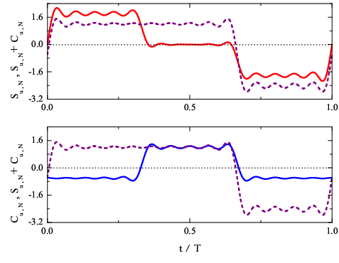
(see Fig. 1, top panel). From the Fourier series of [Eq. (4)], one has four harmonic pairs having frequencies and in each pair:
| (8a) | ||||
| (8b) | ||||
| (8c) | ||||
| (8d) |
We see that the waveforms of the biharmonic expressions (8c) and (8d) do not correspond to that of the biharmonic universal excitation (cf. Eq. (6)), the biharmonic expression (8b) with does but presents a phase difference of with respect to , while the biharmonic expression (8a) with does and is in phase with . Therefore, the compatibility between the exact universal excitation waveform and the biharmonic universal excitation requires that , i.e.,
| (9) |
After defining , Eq. (9) can be put into the form , , for the signs , respectively. The solutions and of the latter algebraic equation lack mathematical sense () and physical sense (, cf. Eq. (5)), respectively. The solutions of the former algebraic equation are . For the only meaningful solution, , one has
| (10) |
Thus, after using Eq. (5), one finally obtains the conditions and for the cases and , respectively. Therefore, the values (or equivalently ) fix the exact universal waveform of the excitation which yields DRT having the same strength but opposite direction in the cases and . It is worth noting that, for these two values of , , the Fourier coefficients of the exact universal excitation satisfy the properties (cf. Eq. (4))
| (11a) | ||||
| (11b) | ||||
| (11c) | ||||
| (11d) | ||||
| (11e) | ||||
| (11f) |
Properties (11a) and (11b) indicate a subtle periodicity of the coefficients, while property (11c) makes explicit the periodic absence of an infinity of coefficients. Remarkably, properties (11d) and (11e) indicate that the harmonic pairs of the types and , respectively, also satisfy the requirement of the biharmonic universal excitation regarding the relative amplitude of the two harmonics of each pair. Notice that property (11d) also shows that the biharmonic universal excitation waveform is present in an infinite series of harmonic pairs. Moreover, property (11f) together with properties (11a), (11b), and (11c) suggest that the complete Fourier series of the exact universal excitation can be understood as the sum of two complementary series: a series consisting only of sine terms containing all the ratcheting effect, and another series consisting only of cosine terms yielding the maximization of the transmitted impulse. Indeed, for the case for instance, one has
| (12) |
where represent the aforementioned complementary series, while denote the corresponding truncated series after terms, respectively (see Fig. 1, middle and bottom panels).


Alternatively, the suitable value of can be calculated from the quantifier of the DSB associated with the shift symmetry of , [cf. Eq. (1)]. To this end, we properly require that the (positive and negative) amplitudes of and a suitable (symmetry-breaking-inducing) biharmonic excitation, for example with [16], should be the same, i.e., , . One thus obtains straightforwardly
| (13) |
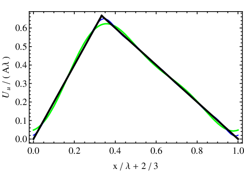
with (and hence ), and where an increase in the deviation of from 1 (unbroken symmetry) indicates an increase in the DSB. One finds that has the value , and presents, as a function of , a single extremum at (see Fig. 2, top panel), and hence the DSB is maximum when [cf. Eqs. (5) and (13)]. As expected from a symmetry analysis, we obtained the same behaviour when using any other alternative form for together with the corresponding suitable values of in each case [16]. In particular, for the other optimal value, corresponding to , one straightforwardly obtains , , and with (and hence ). This value of presents the same dependence on than that corresponding to [Eq. (13)], and hence the DSB is maximum when and the DRT has the same strength but opposite direction to that corresponding to . Therefore, the values (or equivalently ) again fix the exact universal waveform of the excitation as well as the properties of the associated ratchet potential (see Fig. 2, middle and bottom panels). In this regard, it is worth mentioning that the biparametric family of dichotomous driving waveforms predicted in Ref. [20] for optimal enhancement of DRT in overdamped, adiabatic rocking ratchets includes (without indicating that it is a special case) the exact universal waveform of for the particular choice . Also, the exact universal waveform was used (without indicating the reason of its choice) in the experimental realization of a relativistic-flux-quantum-based diode [12]. After calculating the Fourier series of the universal excitation and potential,
| (14) | ||||
| (15) |
where is the spatial period, one obtains the geometric properties of the universal ratchet potential per unit of amplitude and unit of spatial period [Eq. (15); see Fig. 2, bottom panel].


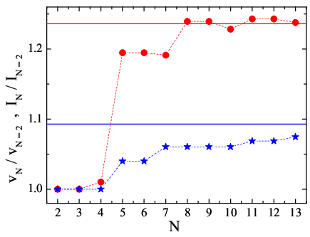
Next, we consider the case and [cf. Eq. (15)], i.e., in Eq. (3), with being the Fourier series of truncated after terms [cf. Eq. (14)]. Our numerical results systematically indicate an overall increase of the maximum value of with the number of terms , while keeping the remaining parameters constant. Moreover, the typical instance shown in Fig. 3 (top panel) indicates that the average velocity (absolute value) quickly increases with , and reaches its asymptotic value for . This behaviour is found to be correlated with that of the impulse per unit of amplitude transmitted by over a half-period,
| (16) |
as expected from the theory of RU [16] (see Fig. 3, bottom panel).

Harmonic excitations.For the sake of completeness, we next explore the standard case [2] in which the two temporal excitations involved are harmonic: , in Eq. (2), i.e.,
| (17) |
in Eq. (3). Leaving aside the effect of noise (an effective change of the potential barrier which is in turn controlled by the DSB mechanism [15]), RU predicts (for ) that the optimal value of the relative amplitude comes from the condition that the amplitude of must be twice as large as that of in Eq. (3) with given by Eq. (17), and the optimal values of the initial phase difference are [16]. Thus, RU predicts the existence of a frequency-dependent optimal value of :
| (18) |
and, equivalently, an optimal frequency for each value of : . Numerical simulations confirmed this prediction over a wide range of frequencies (see Fig. 4, top panel).

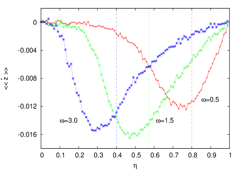
As mentioned above, the numerical estimate of the value at which the average velocity presents an extremum, , is slightly lower than the corresponding value [Eq. (18)], as expected [15] (see Fig. 4, bottom panel). It is worth noting that the property Eq. (18) represents a genuine feature of the back-and-forth travelling potential ratchet [Eq. (2)] which is absent in the case of an overdamped rocking ratchet [15]. Also, this finding is in sharp contrast with the prediction coming from all the earlier theoretical approaches [3,7, 21-23], namely, that the dependence of the average velocity should scale as
| (19) |
which fails to explain the observed phenomenology (cf. Fig. 4). Indeed, this amplitudes catastrophe comes from the assumption that the contributions of the amplitudes of the two harmonic excitations to the average velocity are independent. However, the existence of a universal waveform which optimally enhances DRT implies that the two amplitudes are correlated in the sense mentioned above. It is worth mentioning that the case where the roles played by the harmonic excitations and are interchanged presents different optimal values of the initial phase and a different dependence on the frequency of the optimal value of , and that numerical simulations again confirmed these predictions from RU (see the Appendix for analytical and numerical details). To confirm the aforementioned characteristics of the criticality scenario giving rise to the existence of the exact universal excitation waveform, we compared the ratchet effectiveness of the biharmonic excitation [Eq. (17)] with that of [cf. Eq. (4)] subjected to the requirement that both excitations have the same (positive and negative) amplitudes for each value of . Recall that varying the amplitudes of implies varying the asymmetry parameter , and vice versa [cf. Eq. (5)], whence both and will be -dependent so as to allow a proper comparison of the ratchet effectiveness of these excitations. Indeed, the results shown in Fig. 5 indicate that the DRT strength of the dichotomous excitation is greater than that of the biharmonic excitation over (almost) the entire range of values, i.e., enhancement of DRT occurs when the impulse transmitted is maximum regardless of the DSB of the two excitations. One clearly sees in Fig. 5 that the greater the impulse transmitted, the lower the DSB needed to yield the same strength of DRT, and vice versa, as predicted from the criticality scenario. Note that the noise-induced decrease of the optimal value of with respect to the corresponding deterministic prediction, [; cf. Eq. (18)], is slightly lower when the transmitted impulse is maximum. This provides additional evidence for the impulse being the main quantifier of the driving effectiveness of a periodic excitation. Additionally, robustness of the present universality scenario is also observed when the external periodic excitation is replaced by a chaotic excitation having the same underlying main frequency in its Fourier spectrum (see the Appendix).

Conclusions.–In summary, from the criticality scenario giving rise to ratchet universality we have demonstrated the existence and properties of an exact universal excitation waveform for optimal enhancement of directed ratchet transport by providing two alternative derivations. Our numerical experiments confirmed those findings, as well as revealed other unanticipated properties for the standard case of harmonic excitations in the general context of a driven overdamped Brownian particle subjected to a vibrating periodic potential. The exact universal waveform is the simplest possible (a particular dichotomous waveform), and is far more efficient that its biharmonic approximation, and the waveform of the associated optimal ratchet potential is therefore a particular case of the simplest piecewise waveform as is used, for instance, in a flashing ratchet. Since most models of biological Brownian motors are compatible with a simplified description based on the flashing ratchet, we are tempted to conjecture that the universal optimal ratchet potential could underlie the complex biological machinery operating at the nanoscale as a result of evolutionary processes.
R.C. acknowledges financial support from the Junta de Extremadura (JEx, Spain) through Project No. GR18081 cofinanced by FEDER funds. P.J.M. acknowledges financial support from the Ministerio de Economía y Competitividad (MINECO, Spain) through project FIS2017-87519 cofinanced by FEDER funds and from the Gobierno de Aragón (DGA, Spain) through grant E36_17R to the FENOL group.
I APPENDIX: SUPPLEMENTARY CALCULATION DETAILS AND RESULTS
This Appendix provides details on the energy analysis, the case where the roles of the harmonic excitations are interchanged, and the case where the external periodic excitation is substituted by a chaotic excitation.
I.1 Energy-based analysis
In this subsection we deduce an analytical expression for the mean kinetic energy per unit of mass on averaging over different realizations of noise of a Brownian particle of mass which satisfies the general equation of motion
| (A1) |
where is a potential subject to a lower bound (i.e., ), is a unit-amplitude -periodic function with zero mean, is a Gaussian white noise of zero mean and , and with and being the Boltzmann constant and temperature, respectively. Also, we assume without loss of generality that and redefine here the impulse transmitted by (per unit of amplitude) as
| (A2) |
Equation (A1) has the associated energy equation
| (A3) |
where is the energy function. Integration of Eq. (A3) over the intervals and , , yields
| (A4) | ||||
| (A5) |
respectively, where the second integrals in Eqs. (A4) and (A5) are considered in the Stratonovich sense. After applying the first mean value theorem for integrals [24] to the last integrals on the right-hand sides of Eqs. (A4) and (A5), using Eq. (A2), and recalling that is a zero-mean function, one obtains
| (A6) | ||||
| (A7) | ||||
respectively, where the discrete variables , with and being unknown instants which only have to satisfy the respective relationships and , according to the first mean value theorem for integrals. After adding Eqs. (A6) and (A7) from to and dividing the result by , one obtains
| (A8) |
Upon taking the limit in Eq. (A8), averaging over different realizations of noise, and recalling that the system (A1) is dissipative and that is a stationary random process which cannot contain a shot noise component, one finally obtains
| (A9) |
The following remarks are now in order. First, provides the average of the particle’s velocity when is measured exclusively at certain instants for which has the same sign as the acceleration [cf. Eq. (A1)], i.e., when tends to yield an increase in the particle’s velocity, while does the same when has the opposite sign to , i.e., when tends to yield a decrease in the particle’s velocity. One sees from Eq. (A9) that the effect of the difference on the average kinetic energy per unit of mass is modulated by the impulse per unit of amplitude, while keeping the remaining parameters constant. Second, increasing the noise strength from activates the term , which can be positive or negative. Third, one has and hence Eq. (A9) remains valid in the overdamped limiting case.
I.2 Complementary case of harmonic excitations
Let us consider the case of harmonic excitations in Eq. (2) when the roles of the excitations and are interchanged, i.e., the Langevin equation now reads
| (A10) |
In the reference frame associated with the vibrating potential, one then obtains
| (A11) |
where . Once again, ratchet universality predicts that the optimal value of the relative amplitude comes from the condition that the amplitude of must be twice as large as that of in Eq. (A11), while the optimal values of the initial phase difference are [16]. It therefore predicts the existence of a different (with respect to the case considered above, cf. Eq. (18)) frequency-dependent optimal value of :
| (A12) |
and, equivalently, a different optimal frequency for each value of :
| (A13) |
Numerical simulations (as shown in Fig. 6) confirmed this new prediction over a wide range of frequencies.

I.3 Robustness against chaotic excitations
In this subsection, we study the robustness of the universality scenario against the presence of a bounded chaotic excitation instead of an external periodic excitation. We shall consider the simple case , in Eq. (2), i.e.,
| (A14) |
in Eq. (3), where is a chaotic response of a master system exhibiting the same underlying main frequency, , in its Fourier spectrum [cf. Eq. (17)], but cannot itself yield DRT. The value of is chosen in order for the excitations and to have similar ranges. We considered the following master system (damped driven pendulum)
| (A15) |
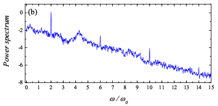
with the parameter values for which the pendulum presents a chaotic attractor irrespective of the initial conditions. Figure 7(a) shows the time series corresponding to the velocity , and Fig. 7(b) shows the corresponding power spectrum which presents its main peak at the frequency . Note the presence of additional peaks at the frequencies , i.e., the underlying periodic solution, , only presents odd harmonics and hence satisfies the shift symmetry with . This means that the function itself cannot yield directed ratchet transport.

We found numerically the same dependence of the average velocity on as in the biharmonic case [Eq. (17)], but with a drastic decrease of the DRT strength (see Fig. 8, top). Indeed, the presence of other noticeable harmonics in the Fourier spectrum of [cf. Fig. 7(b)] yields interferences with the excitation which leads to deviate from the optimal biharmonic approximation [cf. Eq. (10)]. This phenomenon and the inherent noise background lead to losing DRT effectiveness, but without deactivating the DSB mechanism, and also to an additional decrease in the optimal value of with respect to the corresponding deterministic prediction [cf. Eq. (18)]. This robustness is also manifest in the dependence of the average velocity on (see Fig. 8, bottom).

References
- (1) R. P. Feynman, R. B. Leighton, and M. Sands, The Feynman Lectures on Physics (Addison Wesley, Reading, 1966) Vol. 1, Chapt. 46; J. M. R. Parrondo and P. Español, Am. J. Phys. 64, 1125 (1996).
- (2) P. Reimann, Phys. Rep. 361, 57 (2002).
- (3) P. Hänggi and F. Marchesoni, Rev. Mod. Phys. 81, 387 (2009).
- (4) F. Jülicher, A. Ajdari, and J. Prost, Rev. Mod. Phys. 69, 1269 (1997).
- (5) M. Gu and C. M. Rice, Proc. Natl. Acad. Sci. U.S.A. 107, 521 (2010).
- (6) Jing-hui Li, Phys. Rev. E 67, 061110 (2003).
- (7) S. Flach, O. Yevtushenko, and Y. Zolotaryuk, Phys. Rev. Lett. 84, 2358 (2000); S. Denisov, S. Flach, A. A. Ovchinnikov, O. Yevtushenko, and Y. Zolotaryuk, Phys. Rev. E 66, 041104 (2002).
- (8) A. B. Kolton, Phys. Rev. B 75, 020201(R) (2007).
- (9) P. J. Martínez and R. Chacón, Phys. Rev. Lett. 100, 144101 (2008).
- (10) J. L. Mateos, Phys. Rev. Lett. 84, 258 (2000); P. Malgaretti, I. Pagonabarraga, and D. Frenkel, Phys. Rev. Lett. 109, 168104 (2011); A. Wickenbrock, D. Cubero, N. A. Abdul Wahab, P. Phoonthong, and F. Renzoni, Phys. Rev. E 84, 021127 (2011).
- (11) M. Rietmann, R. Carretero-González, and R. Chacón, Phys. Rev. A 83, 053617 (2011).
- (12) G. Carapella and G. Costabile, Phys. Rev. Lett. 87, 077002 (2001); G. Carapella, Phys. Rev. B 63, 054515 (2001).
- (13) F. R. Alatriste and J. L. Mateos, Physica A 372, 263 (2006).
- (14) R. Gommers, S. Bergamini, and F. Renzoni, Phys. Rev. Lett. 95, 073003 (2005).
- (15) P. J. Martínez and R. Chacón, Phys. Rev. E 87, 062114 (2013); 88, 019902(E) (2013); 88, 066102 (2013).
- (16) R. Chacón, J. Phys. A: Math. Theor. 40, F413 (2007); 43, 322001 (2010).
- (17) M. Schiavoni, L. Sánchez-Palencia, F. Renzoni, and G. Grynberg, Phys. Rev. Lett. 90, 094101 (2003); R. Chacón, arXiv:1802.02826 (2018).
- (18) T. Salger et al., Science 326, 1241 (2009).
- (19) V. Berardi, J. Lydon, P. G. Kevrekidis, C. Daraio, and R. Carretero-González, Phys. Rev. E 88, 052202 (2013).
- (20) S. J. Lade, J. Phys. A: Math. Theor. 41, 275103 (2008).
- (21) F. Marchesoni, Phys. Lett. A 119, 221 (1986).
- (22) N. R. Quintero, J. A. Cuesta, and R. Alvarez-Nodarse, Phys. Rev. E 81, 030102(R) (2010); J. A. Cuesta, N. R. Quintero, and R. Alvarez-Nodarse, Phys. Rev. X 3, 041014 (2013).
- (23) S. Denisov, S. Flach, and P. Hänggi, Phys. Rep. 538, 77 (2014).
- (24) Gradshteyn, I. S. & Ryzhik, I. M. Table of Integrals, Series, and Products (Academic Press, 1980).