Wave-particle duality of many-body quantum states

The first-quantization formalism developed in the present section is equivalent to the usual second-quantization approach but highlights the interdependencies between internal and external degrees of freedom, which are at the heart of our understanding of particle distinguishability. We aim at describing $N$ identical bosons or fermions which are prepared in an arbitrary state of their internal ($\mathrm{I}$) degrees of freedom, and expanded over $n$ mutually orthogonal external ($\mathrm{E}$) states (or modes). The single-particle Hilbert space $\mathcal{H}=\mathcal{H}_{\mathrm{E}}\otimes\mathcal{H}_{\mathrm{I}}$ is composed of the $n$-dimensional external Hilbert space $\mathcal{H}_{\mathrm{E}}$ spanned by the orthonormal basis $\{\ket{1},\dots,\ket{n}\}$, tensored with the $m$-dimensional internal Hilbert space $\mathcal{H}_{\mathrm{I}}$ spanned by the orthonormal basis $\{\ket{i_{1}},\dots,\ket{i_{m}}\}$. Note that, while we choose to work with finite-dimensional Hilbert spaces for simplicity, our formalism allows a straightforward extension to include continuous degrees of freedom. For $N$ identical particles, the basis states of $\mathcal{H}^{\otimes N}=\mathcal{H}_{\mathrm{E}}^{\otimes N}\otimes\mathcal{H}_{\mathrm{I}}^{\otimes N}$ are then given as $N$-fold tensor products of single particle basis states. An orthonormal basis of the $n^{N}$-dimensional external Hilbert space $\mathcal{H}_{\mathrm{E}}^{\otimes N}$ is therefore composed of the states

with $\mathcal{E}_{j}\in\{1,\dots,n\}$. In the literature, the $N$-tuple $\vec{\mathcal{E}}$ is commonly called mode assignment list Tichy et al. 2010; Tichy et al. 2012; Tichy 2014; Dittel et al. 2018a; Dittel et al. 2018b. Analogously, an orthonormal basis of the $m^{N}$-dimensional $N$-particle internal Hilbert space $\mathcal{H}_{\mathrm{I}}^{\otimes N}$ is given by states

where $\mathcal{I}_{j}\in\{i_{1},\dots,i_{m}\}$. Note that in Eqs. (13) and (14) each particle is implicitly given a label corresponding to its position in the tensor product. This sort of labeling is characteristic of the first quantization formalism and is unphysical for identical particles. Therefore, we eliminate it by (anti)symmetrization later on.

With an orthonormal basis of $\mathcal{H}^{\otimes N}$ at hand, we can now describe partially distinguishable particles with an arbitrary internal state and a fixed particle occupation in the external modes (the latter is a natural assumption, inspired by a typical experimental scenario, e.g., in photonic circuitry Tillmann et al. 2013; Spagnolo et al. 2014; Carolan et al. 2015; Loredo et al. 2017; Wang et al. 2017). This distribution is specified by the mode occupation list Tichy et al. 2010; Tichy et al. 2012; Tichy 2014; Dittel et al. 2018a; Dittel et al. 2018b $\vec{R}=(R_{1},\dots,R_{n})$, where $R_{j}$ is the number of particles in mode $j$. Since several mode assignment lists $\vec{\mathcal{E}}$ correspond to a given occupation $\vec{R}$, we single out the mode assignment list $\vec{E}\equiv\vec{E}(\vec{R})$ with components listed in non-decreasing order, $E_{1}\leq E_{2}\leq\dots\leq E_{N}$. Other external basis states $\ket{\vec{\mathcal{E}}}$ corresponding to the same mode occupation $\vec{R}$ are then obtained by permutation of the factors of $\ket{\vec{E}}$. The external state of the particles can therefore be written in terms of the states

for $\pi$ a permutation in the symmetric group $\mathrm{S}_{N}$. In short, for each mode occupation $\vec{R}$, there exists a unique basis state $\ket{\vec{E}}$ with elements in non-decreasing order, from which we obtain all basis states $\ket{\vec{\mathcal{E}}}$ associated with $\vec{R}$ by permuting the factors of $\ket{\vec{E}}$.

Regarding the internal degrees of freedom, we impose no restriction on the $N$-particle state, which we write as a general superposition of all internal basis states (14),

This allows us to consider the effects of correlations and mixedness in the internal state (with the index $j$ used below to label different states in a statistical mixture) on many-particle interference in the external degree of freedom. The coefficients $C_{\vec{\mathcal{I}}}^{(j)}$ ultimately determine the distinguishability of the particles Shchesnovich 2015b; Shchesnovich 2016; Shchesnovich and Bezerra 2017. The bosonic (fermionic) state of particles in the external configuration $\vec{R}$ with internal state $\ket{\Omega^{(j)}}$ is then obtained by (anti)symmetrization, i.e. by forming the coherent sum over all permutations (disregarding normalization, for the moment)

where we have introduced the permuted internal basis states

The sign factor is given by $(-1)^{\pi}_{\mathrm{B}}=1$ for bosons and $(-1)^{\pi}_{\mathrm{F}}=\mathrm{sgn}(\pi)$ for fermions, respectively. As apparent from Eq. (17), the (anti)symmetrization of $\ket{\Psi^{(j)}}$ results in the entanglement of the particles’ external and internal degrees of freedom, with a strength which depends on the particles’ internal state. We will elaborate upon this observation further down.

In the case of multiple occupations, i.e. if there is a mode $i$ such that $R_{i}\geq 2$, distinct permutations $\pi\neq\pi^{\prime}$ can lead to the same state $\ket{\vec{E}_{\pi}}=\ket{\vec{E}_{\pi^{\prime}}}$. This defines an equivalence relation $\pi\sim\pi^{\prime}$, and we constitute a set $\Sigma\equiv\Sigma(\vec{R})$ by choosing one representative in each of the $R=N!/(\prod_{j=1}^{n}R_{j}!)$ equivalence classes. Any permutation $\pi\in\mathrm{S}_{N}$ can then be uniquely decomposed as $\pi=\xi\mu$, with $\mu\in\Sigma$ and $\xi\in\mathrm{S}_{\vec{R}}$, where $\mathrm{S}_{\vec{R}}=\mathrm{S}_{R_{1}}\otimes\dots\otimes\mathrm{S}_{R_{n}}$ denotes the subgroup of $\mathrm{S}_{N}$ which leaves $\ket{\vec{E}}$ invariant. In group theoretical terms, $\Sigma$ is a transversal of the set of right cosets of $\mathrm{S}_{\vec{R}}$ in $\mathrm{S}_{N}$, also called right transversal of $\mathrm{S}_{\vec{R}}$ in $\mathrm{S}_{N}$ Baumslag and Chandler 1968. Since each permutation $\mu\in\Sigma$ corresponds to one of the $R$ inequivalent ways of ordering the particles, we refer to $\mu$ as a particle labeling. The normalized state $\ket{\Psi^{(j)}}$ can thus be written as a sum over particle labelings

with

From Eq. (20), one sees that the coefficients $C_{\vec{\mathcal{I}}}^{(j)}$ must be (anti)symmetrized over permutations of bosons (fermions) belonging to the same external mode,

for all $\xi\in\mathrm{S}_{\vec{R}}$ (note that $\vec{\mathcal{I}}_{\xi}=(\mathcal{I}_{\xi(1)},\dots,\mathcal{I}_{\xi(N)})$). For fermions, this enforces Pauli’s exclusion principle Pauli 1925: fermions in the same mode must be in orthogonal internal states. Without loss of generality, we choose the $C_{\vec{\mathcal{I}}}^{(j)}$ to already satisfy this symmetry and obey $\sum_{\vec{\mathcal{I}}}|C_{\vec{\mathcal{I}}}^{(j)}|^{2}=1$, such that the normalized internal states in Eq. (19) read

Finally, states with mixed internal degrees of freedom can be expressed as

where $\ket{\Psi^{(j)}}$ from Eq. (19) appears with probability $q_{j}$, and $\sum_{j}q_{j}=1$.

The state of $N$ fully indistinguishable identical particles is obtained by assigning the same internal state to each particle, e.g. $\ket{\Omega}=\ket{i_{1}}^{\otimes N}$. Fully distinguishable identical particles are obtained when all particles are in mutually orthogonal internal states, such that they can be identified unambiguously, e.g. if $\ket{\Omega}=\ket{i_{1}}\otimes\ket{i_{2}}\otimes\dots\otimes\ket{i_{N}}$.

Before we continue, let us consider a brief example, illustrated in Fig. 3. We consider $N=3$ bosons in $n$ modes with two particles in mode $1$ and one particle in mode $2$, such that $\vec{R}=(2,1,0\dots,0)$, $R=N!/(\prod_{j=1}^{n}R_{j}!)=3$, and $\vec{E}=(1,1,2)$. With $\epsilon$ the identity permutation and permutations given in cycle notation, we have $\mathrm{S}_{\vec{R}}=\{\epsilon,(12)\}$, and find $\Sigma=\{\epsilon,(13),(23)\}$. Note that for $\vec{R}=(2,1,0,\dots,0)$ and $\pi\in\mathrm{S}_{3}$, there are three distinct right cosets $\mathrm{S}_{\vec{R}}\pi$ of $\mathrm{S}_{\vec{R}}$ in $\mathrm{S}_{3}$, $\mathrm{S}_{\vec{R}}\epsilon=\mathrm{S}_{\vec{R}}(12)=\{\epsilon,(12)\}$, $\mathrm{S}_{\vec{R}}(13)=\mathrm{S}_{\vec{R}}(132)=\{(13),(132)\}$, and $\mathrm{S}_{\vec{R}}(23)=\mathrm{S}_{\vec{R}}(123)=\{(23),(123)\}$. The right transversal $\Sigma$ is then obtained by choosing one element of each distinct right coset, e.g. $\Sigma=\{\epsilon,(13),(23)\}$. With the help of $\Sigma$ we can extract the subset of external basis states needed in Eq. (19), $\{\ket{\vec{E}_{\mu}}\}_{\mu\in\Sigma}=\{\ket{1,1,2},\ket{2,1,1},\ket{1,2,1}\}$.

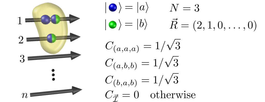
In this example, we consider pure internal states, such that the sum in Eq. (22) consists of just one term and the index $j$ is dropped. Moreover, the single-particle internal Hilbert space is assumed to be of dimension $m=2$ and spanned by the basis $\{\ket{a},\ket{b}\}$. We consider the correlated internal state defined by the choice of coefficients $C_{(a,a,a)}=C_{(a,b,b)}=C_{(b,a,b)}=1/\sqrt{3}$, and $C_{\vec{\mathcal{I}}}=0$ otherwise. These coefficients satisfy the required symmetry $C_{\vec{\mathcal{I}}_{\xi}}=C_{\vec{\mathcal{I}}}$ for all $\xi\in\mathrm{S}_{\vec{R}}=\mathrm{S}_{2}\otimes\mathrm{S}_{1}\otimes\mathrm{S}_{0}\otimes\dots=\{\epsilon,(12)\}$, where permutations $\xi\in\mathrm{S}_{\vec{R}}$ only permute particles in the same mode. The internal state (16) then reads

The symmetrized pure state (19) is obtained by combining the external states $\ket{\vec{E}_{\mu}}$ and the internal states $\ket{\Omega_{\mu}}$ for all particle labelings $\mu\in\Sigma$,

where the summands in the first, second and third row correspond to $\mu=\epsilon$, $\mu=(13)$ and $\mu=(23)$, respectively. One can easily verify that this state is symmetric under the exchange of any two particles, as required for a state of many bosons.

We now consider the reduced external and internal states of systems of partially distinguishable particles, to reveal the connection to the single-particle case described in section II. First, let us rewrite the state (22) in the same form as Eq. (2), with the help of Eq. (19):

In general, the (anti)symmetrized state (24) shows entanglement between external and internal degrees of freedom. As we show below, this entanglement can be used to characterize the distinguishability of the particles Stanisic and Turner 2018, and to quantify the many-particle wave character.

We first consider the reduced external state obtained by tracing out the internal state-space in Eq. (24),

with elements

[compare with Eqs. (3) and (4)]. In the basis $\{\ket{\vec{\mathcal{E}}}\}_{\vec{\mathcal{E}}}$, the off-diagonal elements of $\rho_{\mathrm{E}}$ are thus determined by particle distinguishability via the overlaps $\langle\Omega_{\nu}^{(j)}\vphantom{\Omega_{\mu}^{(j)}}|\Omega_{\mu}^{(j)}\vphantom{\Omega_{\nu}^{(j)}}\rangle$ for different particle labelings $\mu\neq\nu$. Note that in Refs. Shchesnovich 2015a; Shchesnovich 2015b; Shchesnovich and Bezerra 2017, particle distinguishability is described by the so called $J$-matrix which, in our formalism, has elements $J_{\nu,\mu}=R[\rho_{\mathrm{E}}]_{\mu,\nu}=\sum_{j}q_{j}\langle\Omega_{\nu}^{(j)}\vphantom{\Omega_{\mu}^{(j)}}|\Omega_{\mu}^{(j)}\vphantom{\Omega_{\nu}^{(j)}}\rangle$. On the other hand, for the description of particles in an internal product state, Ref. Tichy 2015 introduced the distinguishability matrix $\mathcal{S}$. In this case, we have $\langle\Omega_{\nu}\vphantom{\Omega_{\mu}}|\Omega_{\mu}\vphantom{\Omega_{\nu}}\rangle=\prod_{i=1}^{N}\mathcal{S}_{\nu(i),\mu(i)}$ [see also Ref. Chin and Huh 2018].

In the case of distinguishable particles $(\mathrm{D})$, each particle is in a distinct orthogonal internal state and these overlaps vanish. As a result, the reduced external state is maximally mixed,

On the other hand, perfectly indistinguishable bosons (fermions) share the same pure internal state, such that $\langle\Omega_{\nu}^{(j)}\vphantom{\Omega_{\mu}^{(j)}}|\Omega_{\mu}^{(j)}\vphantom{\Omega_{\nu}^{(j)}}\rangle=1$, for all $j$ and $\mu,\nu\in\Sigma$. Therefore, the external state is pure and given by

with

The coherences (off-diagonal elements) of the reduced external state (25) thus reflect the indistinguishability of the particles. As we show in Eq. (44) in Sec. IV below, these coherences are at the origin of many-particle interference in the external degrees of freedom and are therefore constitutive of the particles’ wave character. On a related note, the purity of $\rho_{\mathrm{E}}$, which, by virtue of Eqs. (27) and (28), quantifies the separability of internal and external degrees of freedom, is, in turn, a marker of indistinguishability. In the case of indistinguishable particles, the particles’ internal and external degrees of freedom are uncorrelated and $\rho_{\mathrm{E}}$ appears pure. On the other hand, for fully distinguishable particles, with each particle in a distinct orthogonal internal state, the particles’ internal and external degrees of freedom are maximally correlated, and the reduced state $\rho_{\mathrm{E}}^{\mathrm{D}}$ is maximally mixed on its support. We pursue this direction further in the next section.

Let us now consider the reduced internal state by tracing over the external state-space in Eq. (24):

The result is a balanced mixture of the internal states

which correspond to different particle labelings $\mu$ [note the close analogy with Eq. (7)]. In the case of indistinguishable particles, the internal states $\rho_{\mathrm{I}}^{\mu}$ are equal for all particle labelings $\mu\in\Sigma$ and cannot be discriminated. In contrast, for distinguishable particles and pure internal states, such that the sum in (31) reduces to a single term, the states $\rho_{\mathrm{I}}^{\mu}$ can be discriminated with certainty, i.e. $\rho_{\mathrm{I}}^{\mu}$ and $\rho_{\mathrm{I}}^{\nu}$ have support on orthogonal subspaces for $\mu\neq\nu$. Therefore, different particle labelings can be told apart from each other. The ability to discriminate different labelings thus constitutes a particle-like property of the many-body state. Note, however, that, for mixed internal states, even if every term in the mixture corresponds to fully distinguishable particles, perfect discrimination of the labellings might not be possible.

In the previous section, we identified the magnitude of the coherences of the reduced external state (25) with the many-particle wave character, and the ability to discriminate the internal states (31) with the constituents’ particle character. Based on these observations, we now define normalized measures that quantify these attributes.

So far, for a state of many partially distinguishable particles, we related the measures $\mathcal{W}_{\mathrm{C}}$ and $\mathcal{W}_{\mathrm{P}}$ [see Eqs. (32) and (33)] to its many-particle wave character, and $\mathcal{P}_{\mathrm{T}}$ and $\mathcal{P}_{\mathrm{F}}$ [see Eqs. (37) and (40)] to its particle character. These measures quantify the ability of particles to display many-particle interference on the one hand, and the possibility of individually identifying and tracking them, on the other hand. Wave-particle duality relations state that both properties cannot be fully realized in the same state: the amount of wave character limits the amount of particle character, and vice versa. For $\mathcal{P}_{\mathrm{F}}$ and $\mathcal{W}_{\mathrm{P}}$, this is quantitatively expressed by

which we prove in Appendix D. This constitutes a wave-particle duality relation since it saturates for pure internal states. By the hierarchies (34) and (41) (which do not necessarily saturate for pure internal states), we additionally find complementarity relations between all combinations of the above defined wave and particle measures:

for $\mathcal{P}\in\{\mathcal{P}_{\mathrm{T}},\mathcal{P}_{\mathrm{F}}\}$ and $\mathcal{W}\in\{\mathcal{W}_{\mathrm{C}},\mathcal{W}_{\mathrm{P}}\}$. Interestingly, the complementarity relation (43) saturates for pure internal states for the wave measure $\mathcal{W}_{\mathrm{P}}$, but not for $\mathcal{W}_{\mathrm{C}}$. While the former quantifies the correlations between internal and external degrees of freedom independently of the chosen basis via their entanglement, the latter measures these correlations via the coherence of $\rho_{\mathrm{E}}$ in the chosen external basis. Therefore, the entanglement-based measure $\mathcal{W}_{\mathrm{P}}$ seems to have a more fundamental status, while the coherence-based one $\mathcal{W}_{\mathrm{C}}$ might be more suited to describe measurements performed in a specific basis.

All complementarity relations (43) and their dependence on the mixedness of the internal state are illustrated via a numerical example in Fig. 4. We consider $N=3$ particles occupying distinct modes, with external and internal single-particle Hilbert spaces of dimension $n=m=4$. We generate $300$ random states of partially distinguishable particles by mixing $l=1,3,10$ or $30$ different pure internal states (21) [see Eq. (22)]. The probabilities $q_{j}$ in (22) are randomly chosen according to a uniform probability distribution in the range $q_{j}\in[0,1]$, and normalized such that $\sum_{j=1}^{l}q_{j}=1$. Many-particle distinguishability is encoded in the coefficients $C_{\vec{\mathcal{I}}}^{(j)}=r_{\vec{\mathcal{I}}}^{(j)}\exp(i\varphi_{\vec{\mathcal{I}}}^{(j)})$ – which enter through (21). To fairly distribute the $300$ generated states over all possible levels of partial distinguishability, for the internal states of the $k$th state (with $0\leq k\leq 300$), we uniformly pick $r_{\vec{\mathcal{I}}}^{(j)}\in[1-k/300,1]$ and $\varphi_{\vec{\mathcal{I}}}^{(j)}\in[-\pi k/300,\pi k/300]$ for each $\vec{\mathcal{I}}$ and each pure state $j$. This results in $lm^{N}=l4^{3}$ different coefficients $C_{\vec{\mathcal{I}}}^{(j)}$, which are then appropriately normalized, such that $\sum_{\vec{\mathcal{I}}}|C_{\vec{\mathcal{I}}}^{(j)}|^{2}=1$ for each $j=1,\dots,l$. Note that no symmetrization of the coefficients is required since we consider at most singly occupied modes.

In Figs. 4(a-d) and 4(e-h), we plot the squared wave character quantifiers $\mathcal{W}_{\mathrm{C}}^{2}$ and $\mathcal{W}_{\mathrm{P}}^{2}$ against the squared particle character quantifiers $\mathcal{P}_{\mathrm{F}}^{2}$ and $\mathcal{P}_{\mathrm{T}}^{2}$, for $\l=1,3,10,$ and $30$. Pure internal states ($l=1$) come close to saturating the upper bound for all complementarity relations (43), as shown in Figs. 4(a) and (e). In particular, the saturation of Eq. (42) is evident from Fig. 4(a). However, for stronger mixing of the internal states, i.e. for increasing $l$, the sum of the squared quantifiers of complementary many-particle properties tends to move away from the upper bound which, by Eq. (41), is stronger for $\mathcal{P}_{\mathrm{T}}^{2}$ as compared to $\mathcal{P}_{\mathrm{F}}^{2}$ [compare Figs. 4(a-d) with Figs. 4(e-h)]. Note that while full wave character quantifiers imply vanishing particle character quantifiers, the converse is not true. Indeed, mixing of internal states can reduce the particle character quantifiers [see the discussion below Eq. (31)], such that states with a low wave character can also have low particle character. For all sampled states, we find very similar values for both wave character quantifiers. As shown by the zooms in Fig. (4)(f), the difference between $\mathcal{W}_{\mathrm{P}}^{2}$ and $\mathcal{W}_{\mathrm{C}}^{2}$ tends to increase with more pronounced particle character, which can be traced back to inhomogeneities in the moduli of the off-diagonal elements of $\rho_{\mathrm{E}}$ [see Appendix B].

Let us now return to the analogy between many-particle complementarity as summarized by (43) and the double-slit experiment discussed in Sec. II. First of all, the common state (2) of particle and detector is structurally very similar to the many-body state (24) of external and internal degrees of freedom. In both cases, the weaker the entanglement between the subsystems, the more pronounced the wave character of the state. This observation has its direct counterpart in the congruent structure of the wave character quantifiers in Eqs. (6) and (33). Consistently, the wave character is related to the coherences of the reduced single-particle state by (5), and of the reduced many-particle external state by (32). The latter, however, leaves room for a much more subtle quantum-classical transition than the former, due to the many degrees of freedom involved.

Likewise, the particle character is determined by the ability to discriminate the states (7) of the which-path detectors in the single-particle case and the many-body internal states (30) in case of partially distinguishable particles. To quantify the particle character, concepts imported from quantum state discrimination lead to a generalization of Eqs. (9) and (10) by  (37) and (40). This deep analogy then results in the many-body generalization (43) of the single particle duality relation (12). For the sake of clarity, all character measures and complementarity relations presented in Secs. II and III are summarized in Table 1.

In Sec. III.3.2, we defined the measures $\mathcal{P}_{\mathrm{T}}$ and $\mathcal{P}_{\mathrm{F}}$ [see Eqs. (37) and (40)] to quantify the many-body state’s particle character. These measures are based on the formal discrimination of different particle labelings $\mu\in\Sigma$ by comparison of the associated internal states $\rho_{\mathrm{I}}^{\mu}$ from Eq. (31). We now show that different particle labelings can equivalently be discriminated by comparing common states, of external and internal degrees of freedom, that differ by an initial permutation of the internal states. Therefore, instead of the unpermuted internal many-particle states $\ket{\Omega^{(j)}}$ from Eq. (16), we consider the internal states $\ket{\Omega_{\kappa}^{(j)}}$ permuted according to $\kappa\in\Sigma$ [see Eq. (21)]. While the unpermuted common state $\rho$ of external and internal degrees of freedom is given in Eq. (24), the permuted states read

Here, the subscript $\kappa\mu$ in $\ket{\Omega_{\kappa\mu}^{(j)}}$ refers to a composition of permutations, with permutation $\kappa$ and $\mu$ arising due to the initially permuted internal states and the symmetrization of the many-particle state, respectively.

In Appendix E, we prove the equality of the distances

and of the fidelities

with $\rho^{\kappa}$ and $\rho_{\mathrm{I}}^{\kappa}$ from Eq. (50) and (31), respectively. Thus, the discrimination of different particle labelings $\kappa$ can be performed equally well by comparison of the internal states $\rho_{\mathrm{I}}^{\kappa}$, or of the permuted common states $\rho^{\kappa}$. We therefore investigate how the outcomes of interference experiments as sketched in Fig. (5) differ for permuted states. This will lead us to classical counterparts of the measures $\mathcal{P}_{\mathrm{T}}$ and $\mathcal{P}_{\mathrm{F}}$ of the particle character, evaluated on the output counting statistics, which also obey complementarity relations of the form (43).

Let us denote by $\rho_{\mathrm{E}}^{\kappa}$ the reduced external state of the permuted state, $\rho_{\mathrm{E}}^{\kappa}=\mathrm{Tr}_{\mathrm{I}}\left(\rho^{\kappa}\right)$, and by $P_{\mathcal{M}}^{\kappa}$ the probability distribution obtained when $\rho^{\kappa}$ is used as input in the experiment depicted in Fig. 5. As we prove in Appendix F, for two permutations $\kappa\neq\tau$, the classical distances between the corresponding output probability distributions are bounded by the magnitude of the corresponding off-diagonal element of $\rho_{\mathrm{E}}$,

References

- Bohr (1935) N. Bohr, Can quantum-mechanical description of physical reality be considered complete?, Phys. Rev. 48, 696 (1935).
- Bohr (1949) N. Bohr, Discussion with Einstein on epistemological problems in atomic physics, in The Library of Living Philosophers, Volume 7. Albert Einstein: Philosopher-Scientist, edited by P. A. Schilpp (Open Court, 1949) pp. 199–241.
- Wootters and Zurek (1979) W. K. Wootters and W. H. Zurek, Complementarity in the double-slit experiment: Quantum nonseparability and a quantitative statement of Bohr’s principle, Phys. Rev. D 19, 473 (1979).
- Greenberger and Yasin (1988) D. M. Greenberger and A. Yasin, Simultaneous wave and particle knowledge in a neutron interferometer, Phys. Lett. A 128, 391 (1988).
- Mandel (1991) L. Mandel, Coherence and indistinguishability, Opt. Lett. 16, 1882 (1991).
- Jaeger et al. (1995) G. Jaeger, A. Shimony, and L. Vaidman, Two interferometric complementarities, Phys. Rev. A 51, 54 (1995).
- Englert (1996) B.-G. Englert, Fringe visibility and which-way information: An inequality, Phys. Rev. Lett. 77, 2154 (1996).
- Dürr (2001) S. Dürr, Quantitative wave-particle duality in multibeam interferometers, Phys. Rev. A 64, 042113 (2001).
- Bimonte and Musto (2003a) G. Bimonte and R. Musto, Comment on “quantitative wave-particle duality in multibeam interferometers”, Phys. Rev. A 67, 066101 (2003a).
- Bimonte and Musto (2003b) G. Bimonte and R. Musto, On interferometric duality in multibeam experiments, J. Phys. A: Math. Gen. 36, 11481 (2003b).
- Englert et al. (2008) B.-G. Englert, D. Kaszlikowski, L. C. Kwek, and W. H. Chee, Wave-particle duality in multi-path interferometers: General concepts and three-path interferometers, Int. J. Quantum Inform. 06, 129 (2008).
- Siddiqui and Qureshi (2015) A. M. Siddiqui and T. Qureshi, Three-slit interference: A duality relation, Prog. Theor. Exp. Phys. 2015, 083A02 (2015).
- Bera et al. (2015) M. N. Bera, T. Qureshi, M. A. Siddiqui, and A. K. Pati, Duality of quantum coherence and path distinguishability, Phys. Rev. A 92, 012118 (2015).
- Bagan et al. (2016) E. Bagan, J. A. Bergou, S. S. Cottrell, and M. Hillery, Relations between coherence and path information, Phys. Rev. Lett. 116, 160406 (2016).
- Coles (2016) P. J. Coles, Entropic framework for wave-particle duality in multipath interferometers, Phys. Rev. A 93, 062111 (2016).
- Qureshi and Siddiqui (2017) T. Qureshi and M. A. Siddiqui, Wave–particle duality in -path interference, Ann. Phys. 385, 598 (2017).
- Bagan et al. (2018) E. Bagan, J. Calsamiglia, J. A. Bergou, and M. Hillery, Duality games and operational duality relations, Phys. Rev. Lett. 120, 050402 (2018).
- Dürr et al. (1998) S. Dürr, T. Nonn, and G. Rempe, Fringe visibility and which-way information in an atom interferometer, Phys. Rev. Lett. 81, 5705 (1998).
- Mei and Weitz (2001) M. Mei and M. Weitz, Controlled decoherence in multiple beam Ramsey interference, Phys. Rev. Lett. 86, 559 (2001).
- Peng et al. (2003) X. Peng, X. Zhu, X. Fang, M. Feng, M. Liu, and K. Gao, An interferometric complementarity experiment in a bulk nuclear magnetic resonance ensemble, J. Phys. A: Math. Gen. 36, 2555 (2003).
- Hornberger et al. (2003) K. Hornberger, S. Uttenthaler, B. Brezger, L. Hackermüller, M. Arndt, and A. Zeilinger, Collisional decoherence observed in matter wave interferometry, Phys. Rev. Lett. 90, 160401 (2003).
- Hackermüller et al. (2004) L. Hackermüller, K. Hornberger, B. Brezger, A. Zeilinger, and M. Arndt, Decoherence of matter wave by thermal emission of radiatoin, Nature 427, 711 (2004).
- Arndt et al. (2005) M. Arndt, K. Hornberger, and A. Zeilinger, Probing the limits of the quantum world, Phys. World 18, 35 (2005).
- Schwindt et al. (1999) P. D. D. Schwindt, P. G. Kwiat, and B.-G. Englert, Quantitative wave-particle duality and nonerasing quantum erasure, Phys. Rev. A 60, 4285 (1999).
- Jacques et al. (2008) V. Jacques, E. Wu, F. Grosshans, F. Treussart, P. Grangier, A. Aspect, and J.-F. Roch, Delayed-choice test of quantum complementarity with interfering single photons, Phys. Rev. Lett. 100, 220402 (2008).
- Yuan et al. (2018) Y. Yuan, Z. Hou, Y.-Y. Zhao, H.-S. Zhong, G.-Y. Xiang, C.-F. Li, and G.-C. Guo, Experimental demonstration of wave-particle duality relation based on coherence measure, Opt. Express 26, 4470 (2018).
- Brune et al. (1996) M. Brune, E. Hagley, J. Dreyer, X. Maître, A. Maali, C. Wunderlich, J. M. Raimond, and S. Haroche, Observing the progressive decoherence of the “meter” in a quantum measurement, Phys. Rev. Lett. 77, 4887 (1996).
- Hong et al. (1987) C. K. Hong, Z. Y. Ou, and L. Mandel, Measurement of subpicosecond time intervals between two photons by interference, Phys. Rev. Lett. 59, 2044 (1987).
- Shih and Alley (1988) Y. H. Shih and C. O. Alley, New type of Einstein-Podolsky-Rosen-Bohm experiment using pairs of light quanta produced by optical parametric down conversion, Phys. Rev. Lett. 61, 2921 (1988).
- Tichy et al. (2010) M. C. Tichy, M. Tiersch, F. de Melo, F. Mintert, and A. Buchleitner, Zero-transmission law for multiport beam splitters, Phys. Rev. Lett. 104, 220405 (2010).
- Mayer et al. (2011) K. Mayer, M. C. Tichy, F. Mintert, T. Konrad, and A. Buchleitner, Counting statistics of many-particle quantum walks, Phys. Rev. A 83, 062307 (2011).
- Cohen-Tannoudji et al. (1973) C. Cohen-Tannoudji, B. Diu, and F. Laloë, Mecanique quantique II (Hermann, editeurs des sciences et des arts, Paris, 1973).
- Ra et al. (2013) Y.-S. Ra, M. C. Tichy, H.-T. Lim, O. Kwon, F. Mintert, A. Buchleitner, and Y.-H. Kim, Nonmonotonic quantum-to-classical transition in multiparticle interference, Proc. Natl. Acad. Sci. U.S.A. 110, 1227 (2013).
- Shchesnovich (2014) V. S. Shchesnovich, Sufficient condition for the mode mismatch of single photons for scalability of the boson-sampling computer, Phys. Rev. A 89, 022333 (2014).
- de Guise et al. (2014) H. de Guise, S.-H. Tan, I. P. Poulin, and B. C. Sanders, Coincidence landscapes for three-channel linear optical networks, Phys. Rev. A 89, 063819 (2014).
- Shchesnovich (2015a) V. S. Shchesnovich, Partial indistinguishability theory for multiphoton experiments in multiport devices, Phys. Rev. A 91, 013844 (2015a).
- Tichy (2015) M. C. Tichy, Sampling of partially distinguishable bosons and the relation to the multidimensional permanent, Phys. Rev. A 91, 022316 (2015).
- Shchesnovich (2015b) V. S. Shchesnovich, Tight bound on the trace distance between a realistic device with partially indistinguishable bosons and the ideal BosonSampling, Phys. Rev. A 91, 063842 (2015b).
- Laibacher and Tamma (2015) S. Laibacher and V. Tamma, From the physics to the computational complexity of multiboson correlation interference, Phys. Rev. Lett. 115, 243605 (2015).
- Tamma and Laibacher (2015) V. Tamma and S. Laibacher, Multiboson correlation interferometry with arbitrary single-photon pure states, Phys. Rev. Lett. 114, 243601 (2015).
- Tillmann et al. (2015) M. Tillmann, S.-H. Tan, S. E. Stoeckl, B. C. Sanders, H. de Guise, R. Heilmann, S. Nolte, A. Szameit, and P. Walther, Generalized multiphoton quantum interference, Phys. Rev. X 5, 041015 (2015).
- Shchesnovich and Bezerra (2017) V. S. Shchesnovich and M. E. O. Bezerra, Collective phases of identical particle interfering on linear multiports, arXiv: 1707:03893v2 (2017).
- Shchesnovich (2017) V. S. Shchesnovich, Partial distinguishability and photon counting probabilities in linear multiport devices, arXiv: 1712:03191:v2 (2017).
- Walschaers (2018) M. Walschaers, Statistical Benchmarks for Quantum Transport in Complex Systems: From Characterisation to Design, Springer Theses (Springer International Publishing, 2018).
- Khalid et al. (2018) A. Khalid, D. Spivak, B. C. Sanders, and H. de Guise, Permutational symmetries for coincidence rates in multimode multiphotonic interferometry, Phys. Rev. A 97, 063802 (2018).
- Stanisic and Turner (2018) S. Stanisic and P. S. Turner, Discriminating distinguishability, arXiv: 1806:01236 (2018).
- Knill et al. (2001) E. Knill, R. Laflamme, and G. J. Milburn, A scheme for efficient quantum computation with linear optics, Nature 409, 46 (2001).
- O’Brien (2007) J. L. O’Brien, Optical quantum computing, Science 318, 1567 (2007).
- Aaronson and Arkhipov (2013) S. Aaronson and A. Arkhipov, The computational complexity of linear optics, Theory of Comput. 9, 143 (2013).
- O’Brien et al. (2003) J. L. O’Brien, G. J. Pryde, A. G. White, T. C. Ralph, and D. Branning, Demonstration of an all-optical quantum controlled-not gate, Nature 426, 264 (2003).
- Franson et al. (2003) J. D. Franson, B. C. Jacobs, and T. B. Pittman, Experimental demonstration of quantum logic operations using linear optical elements, Fortschr. Phys. 51, 369 (2003).
- Gasparoni et al. (2004) S. Gasparoni, J.-W. Pan, P. Walther, T. Rudolph, and A. Zeilinger, Realization of a photonic controlled-not gate sufficient for quantum computation, Phys. Rev. Lett. 93, 020504 (2004).
- Crespi et al. (2013) A. Crespi, R. Osellame, R. Ramponi, D. J. Brod, E. F. Galvão, N. Spagnolo, C. Vitelli, E. Maiorino, P. Mataloni, and F. Sciarrino, Integrated multimode interferometers with arbitrary designs for photonic boson sampling, Nat. Photonics 7, 545 (2013).
- Broome et al. (2013) M. A. Broome, A. Fedrizzi, S. Rahimi-Keshari, J. Dove, S. Aaronson, T. C. Ralph, and A. G. White, Photonic boson sampling in a tunable circuit, Science 339, 794 (2013).
- Tillmann et al. (2013) M. Tillmann, B. Dakić, R. Heilmann, S. Nolte, A. Szameit, and P. Walther, Experimental boson sampling, Nat. Photonics 7, 540 (2013).
- Wang et al. (2017) H. Wang, Y. He, Y.-H. Li, Z.-E. Su, B. Li, H.-L. Huang, X. Ding, M.-C. Chen, C. Liu, J. Qin, J.-P. Li, Y.-M. He, C. Schneider, M. Kamp, C.-Z. Peng, S. Höfling, C.-Y. Lu, and J.-W. Pan, High-efficiency multiphoton boson sampling, Nat. Photonics 11, 361 (2017).
- Kaufman et al. (2014) A. M. Kaufman, B. J. Lester, C. M. Reynolds, M. L. Wall, M. Foss-Feig, K. R. A. Hazzard, A. M. Rey, and C. A. Regal, Two-particle quantum interference in tunnel-coupled optical tweezers, Science 345, 306 (2014).
- Preiss et al. (2015) P. M. Preiss, R. Ma, M. E. Tai, A. Lukin, M. Rispoli, P. Zupancic, Y. Lahini, R. Islam, and M. Greiner, Strongly correlated quantum walks in optical lattices, Science 347, 1229 (2015).
- Kaufman et al. (2016) A. M. Kaufman, M. E. Tai, A. Lukin, M. Rispoli, R. Schittko, P. M. Preiss, and M. Greiner, Quantum thermalization through entanglement in an isolated many-body system, Science 353, 794 (2016).
- Zeiher et al. (2017) J. Zeiher, J. y Choi, A. Rubio-Abadal, T. Pohl, R. van Bijnen, I. Bloch, and C. Gross, Coherent many-body spin dynamics in a long-range interacting ising chain, Phys. Rev. X 7, 041063 (2017).
- Gross and Bloch (2017) C. Gross and I. Bloch, Quantum simulations with ultracold atoms in optical lattices, Science 357, 995 (2017).
- Bergschneider et al. (2018) A. Bergschneider, V. M. Klinkhamer, J. H. Becher, R. Klemt, L. Palm, G. Zürn, S. Jochim, and P. M. Preiss, Correlation and entanglement in an itinerant quantum system, arXiv: 1807.06405 (2018).
- Kaufman et al. (2018) A. M. Kaufman, M. C. Tichy, F. Mintert, A. M. Rey, and C. A. Regal, The Hong–Ou–Mandel effect with atoms (Academic Press, 2018) pp. 377 – 427.
- Preiss et al. (2019) P. M. Preiss, J. H. Becher, R. Klemt, V. Klinkhamer, A. Bergschneider, N. Defenu, and S. Jochim, High-contrast interference of ultracold fermions, Phys. Rev. Lett. 122, 143602 (2019).
- Nielsen and Chuang (2011) M. A. Nielsen and I. L. Chuang, Quantum Computation and Quantum Information: 10th Anniversary Edition, 10th ed. (Cambridge University Press, New York, NY, USA, 2011).
- Fuchs and van de Graaf (1999) C. A. Fuchs and J. van de Graaf, Cryptographic distinguishability measures for quantum-mechanical states, IEEE Trans. Inf. Theory 45, 1216 (1999).
- Helstrom (1976) C. W. Helstrom, Quantum detection and estimation theory (Academic Press New York, 1976).
- Sacchi (2005) M. F. Sacchi, Optimal discrimination of quantum operations, Phys. Rev. A 71, 062340 (2005).
- Spehner (2014) D. Spehner, Quantum correlations and distinguishability of quantum states, J. Math. Phys. 55, 075211 (2014).
- Rudolph et al. (2003) T. Rudolph, R. W. Spekkens, and P. S. Turner, Unambiguous discrimination of mixed states, Phys. Rev. A 68, 010301 (2003).
- Feng et al. (2004) Y. Feng, R. Duan, and M. Ying, Unambiguous discrimination between mixed quantum states, Phys. Rev. A 70, 012308 (2004).
- Tichy et al. (2012) M. C. Tichy, M. Tiersch, F. Mintert, and A. Buchleitner, Many-particle interference beyond many-boson and many-fermion statistics, New J. Phys. 14, 093015 (2012).
- Tichy (2014) M. C. Tichy, Interference of identical particles from entanglement to boson-sampling, Journal of Physics B: Atomic, Molecular and Optical Physics 47, 103001 (2014).
- Dittel et al. (2018a) C. Dittel, G. Dufour, M. Walschaers, G. Weihs, A. Buchleitner, and R. Keil, Totally destructive many-particle interference, Phys. Rev. Lett. 120, 240404 (2018a).
- Dittel et al. (2018b) C. Dittel, G. Dufour, M. Walschaers, G. Weihs, A. Buchleitner, and R. Keil, Totally destructive interference for permutation-symmetric many-particle states, Phys. Rev. A 97, 062116 (2018b).
- Spagnolo et al. (2014) N. Spagnolo, C. Vitelli, M. Bentivegna, D. J. Brod, A. Crespi, F. Flamini, S. Giacomini, G. Milani, R. Ramponi, P. Mataloni, R. Osellame, E. F. Galvão, and F. Sciarrino, Experimental validation of photonic boson sampling, Nat. Photonics 8, 615 (2014).
- Carolan et al. (2015) J. Carolan, C. Harrold, C. Sparrow, E. Martín-López, N. J. Russell, J. W. Silverstone, P. J. Shadbolt, N. Matsudai, M. Oguma, M. Itoh, G. D. Marshall, M. G. Thompson, J. C. F. Matthews, T. Hashimoto, J. L. O’Brien, and A. Laing, Universal linear optics, Science 349, 711 (2015).
- Loredo et al. (2017) J. C. Loredo, M. A. Broome, P. Hilaire, O. Gazzano, I. Sagnes, A. Lemaitre, M. P. Almeida, P. Senellart, and A. G. White, Boson sampling with single-photon Fock states from a bright solid-state source, Phys. Rev. Lett. 118, 130503 (2017).
- Shchesnovich (2016) V. S. Shchesnovich, Universality of generalized bunching and efficient assessment of boson sampling, Phys. Rev. Lett. 116, 123601 (2016).
- Baumslag and Chandler (1968) B. Baumslag and B. Chandler, Schaum’s outline of theory and problems of group theory, Schaum’s outline series (McGraw-Hill, New York, 1968) cover title: Theory and problems of group theory.
- Pauli (1925) W. Pauli, Über den Zusammenhang des Abschlusses der Elektronengruppen im Atom mit der Komplexstruktur der Spektren, Z. Physik 31, 765 (1925).
- Chin and Huh (2018) S. Chin and J. Huh, Partial distinguishability as a coherence resource in boson sampling, arXiv: 1807:11187v1 (2018).
- Yao et al. (2016) Y. Yao, G. H. Dong, X. Xiao, and C. P. Sun, Frobenius-norm-based measures of quantum coherence and asymmetry, Sci. Rep. 6 (2016).
- Qiu (2008) D. Qiu, Minimum-error discrimination between mixed quantum states, Phys. Rev. A 77, 012328 (2008).
- Qiu and Li (2010) D. Qiu and L. Li, Minimum-error discrimination of quantum states: Bounds and comparisons, Phys. Rev. A 81, 042329 (2010).
- Ivanovic (1987) I. D. Ivanovic, How to differentiate between non-orthogonal states, Phys. Lett. A 123, 257 (1987).
- Dieks (1988) D. Dieks, Overlap and distinguishability of quantum states, Phys. Lett. A 126, 303 (1988).
- Peres (1988) A. Peres, How to differentiate between non-orthogonal states, Phys. Lett. A 128, 19 (1988).
- Michler et al. (1996) M. Michler, K. Mattle, H. Weinfurter, and A. Zeilinger, Interferometric Bell-state analysis, Phys. Rev. A 53, R1209 (1996).
- Mattle et al. (1996) K. Mattle, H. Weinfurter, P. G. Kwiat, and A. Zeilinger, Dense coding in experimental quantum communication, Phys. Rev. Lett. 76, 4656 (1996).
- Rowe et al. (2012) D. J. Rowe, M. J. Carvalho, and J. Repka, Dual pairing of symmetry and dynamical groups in physics, Reviews of Modern Physics 84, 711 (2012).
- Puchała and Miszczak (2009) Z. Puchała and J. A. Miszczak, Bound on trace distance based on superfidelity, Phys. Rev. A 79, 024302 (2009).
- Miszczak et al. (2009) J. A. Miszczak, Z. Puchała, P. Horodecki, A. Uhlmann, and K. Zyczkowski, Sub- and super-fidelity as bounds for quantum fidelity, Quantum Info. Comput. 9, 103 (2009).