跳到论文正文
W Papers独立论文阅读器 arXiv:1901.02617 论文正文 计算阅读时间 · 0%
引用这篇论文根据当前论文元数据生成,正式投稿前建议核对。


License: arXiv.org perpetual non-exclusive license
arXiv:1901.02617v2 [cond-mat.str-el] 10 Jan 2019
\typearea

12

J. Stat. Phys. 84, 535–653 (1996).

Stability of Ferromagnetism in Hubbard Models
with Nearly-Flat Bands

Hal Tasaki** * Department of Physics, Gakushuin University, Mejiro, Toshima-ku, Tokyo 171-8588, Japan

Whether spin-independent Coulomb interaction in an electron system can be the origin of ferromagnetism has been an open problem for a long time. Recently, a “constructive” approach to this problem has been developed, and the existence of ferromagnetism in the ground states of certain Hubbard models was established rigorously. A special feature of these Hubbard models is that their lowest bands (in the corresponding single-electron problems) are completely flat. Here we study models obtained by adding small but arbitrary translation-invariant perturbation to the hopping Hamiltonian of these flat-band models. The resulting models have nearly-flat lowest bands. We prove that the ferromagnetic state is stable against a single-spin flip provided that Coulomb interaction UU is sufficiently large. (It is easily found that the same state is unstable against a single-spin flip if UU is small enough.) We also prove upper and lower bounds for the dispersion relation of the lowest energy eigenstate with a single flipped spin, which bounds establish that the model has “healthy” spin-wave excitation. It is notable that the (local) stability of ferromagnetism is proved in non-singular Hubbard models, in which we must overcome competition between the kinetic energy and the Coulomb interaction. We also note that this is one of the very few rigorous and robust results which deal with truly nonperturbative phenomena in many electron systems. The local stability strongly suggests that the Hubbard models with nearly flat bands have ferromagnetic ground states. We believe that the present models can be studied as paradigm models for (insulating) ferromagnetism in itinerant electron systems.

1 Introduction

1.1 Background

The origin of strong ferromagnetic ordering observed in some materials has been a mystery in physical science for a long time [29]. Since non-interacting electron systems universally exhibit paramagnetism, the origin of ferromagnetism should be sought in electron-electron interaction. In most solids, however, the dominant part of interaction between electrons is the Coulomb interaction, which is perfectly spin-independent. (See Chapter 32, page 674 of [3] for example.) Therefore we are faced with a very interesting and fundamental problem in theoretical physics to determine whether spin-independent interaction in an itinerant electron system can be the origin of ferromagnetic ordering. This problem is important not only because ferromagnetism is a very common (and useful) phenomenon, but because it focuses on a fundamental role of nonlinear interactions in many-body quantum mechanical systems.

The present work is a continuation of our work [47, 34], where we dealt with the above fundamental problem from a standpoint of “constructive condensed matter physics.” Our goal is to provide concrete models in which the existence of ferromagnetic ordering can be established rigorously. Such models should shed light on mechanisms by which Coulomb interaction generates ferromagnetic ordering.

It was Heisenberg [14] who first realized that ferromagnetism is an intrinsically quantum mechanical phenomenon. In Heisenberg’s approach to ferromagnetism, one starts from the picture that each electron (relevant to magnetism) is almost localized at an atomic orbit. By treating the effect of Coulomb interaction and overlap between nearby atomic orbits in a perturbative manner, Heisenberg concluded that there appears “exchange interaction” between nearby electronic spins which determines magnetic properties of the system.

The validity of the Heisenberg’s picture has been challenged both from theoretical and from physical points of views. (See, for example, [15].) It has been realized that, in most of the situations, the exchange interaction is antiferromagnetic rather than ferromagnetic. Moreover conditions which would justify the basic assumption that electrons can be treated as localized at atomic sites are not well understood11 1 This issue is closely related to the problem of Mott-Hubbard insulators. .

In a different approach to the problem of ferromagnetism, which was originated by Bloch [5], one starts from the quantum mechanical free electron gas, in which electrons are in plane-wave like states. One then treats the effect of Coulomb interaction perturbatively, and tries to find instability against certain magnetic ordering. When combined with the Hartree-Fock approximation (or a mean-field theory), this approach leads to the picture that there is an instability against ferromagnetism when the density of states at the fermi energy and the Coulomb interaction are sufficiently large.

It has been realized, however, that the Hartree-Fock approximation drastically overestimates the tendency towards ferromagnetism, thus predicting the existence of ferromagnetism in many situations where it does not take place. From a theoretical point of view, the approximation is unsatisfactory since it artificially replaces the fundamental S​U​(2)SU(2) symmetry (i.e., rotation symmetry in the spin space) of the electron systems with a discrete 𝐙2{\bf Z}_{2} symmetry. Although there have appeared many improvements of the simple Hartree-Fock theory, this approach does not provide a conclusive answer to the fundamental problem about the origin of ferromagnetism that we raised in the beginning of the present subsection. See, for example, [16] for a review.

1.2 Ferromagnetism in the Hubbard Model

A modern version of the problem about the origin of ferromagnetism was formulated by Kanamori [18], Gutzwiller [12], and Hubbard [17] in 1960’s. (The similar formulation was given earlier, for example, in [41].) They studied simple tight-binding models of electrons with on-site Coulomb interaction22 2 It is sometimes argued that the originally long ranged Coulomb interaction becomes short ranged by the screening effect from electrons in the bands (or orbits) which are not taken into account in the Hubbard model. But it is still true that the assumption that there is only on-site interaction is highly artificial. whose strength is denoted as UU. The model is usually called the Hubbard model. When there is no electron-electron interaction (i.e., U=0U=0), the model exhibits paramagnetism as an inevitable consequence of the Pauli exclusion principle. Among other things, Kanamori, Gutzwiller, and Hubbard asked whether the paramagnetism found for U=0U=0 can be converted into ferromagnetism when there is a sufficiently large Coulomb interaction UU. This is a concrete formulation of the fundamental problem that we raised in the opening of the previous subsection.

It is worth noting that the on-site Coulomb interaction itself is completely independent of electronic spins, and does not favor any magnetic ordering. Therefore one does not find any terms in the Hubbard Hamiltonian which explicitly favor ferromagnetism (or any other ordering). Our theoretical goal will be to show that magnetic ordering arises as a consequence of subtle interplay between kinetic motion of electrons and the short-ranged Coulomb interaction. It is interesting to compare the situation with that in spin systems, where one is often given a Hamiltonian which favors some kind of magnetic ordering, and the major task is to investigate if such ordering really takes place. We can say that the Hubbard model formulation goes deeper into fundamental mechanisms of magnetism than that of spin systems. It offers a challenging problem to theoretical physicists to derive magnetic interaction from models which do not explicitly contain such interactions. Perhaps the best justification of the Hubbard model as a standard model of itinerant electron systems comes from such a theoretical consideration, rather than its accuracy in modeling narrow band electron systems. See also the introduction of [34, 35, 43] for discussions about ferromagnetism in the Hubbard model.

We stress that ferromagnetism is not a universal property of the Hubbard model. The Hubbard model is believed to exhibit various phenomena including paramagnetism, antiferromagnetism, ferrimagnetism, ferromagnetism, or superconductivity, depending on various conditions. Such drastic “non-universality” of the model motivated us to take the present “constructive” approach rather than to prove theorems which apply to general Hubbard models.

The problem of ferromagnetism in the Hubbard model was extensively studied by using various heuristic methods. The Hartree-Fock approximation discussed above leads one to the so called Stoner criterion. It says that the Hubbard model exhibits ferromagnetism if one has U​DF>1UD_{\rm F}>1, where DFD_{\rm F} is the density of states of the corresponding single-electron problem measured at the fermi level (of the corresponding non-interacting system). Although the criterion cannot be trusted literally, it guides us to look for ferromagnetism in models with not too small UU and/or large density of states.

The first rigorous result about ferromagnetism in the Hubbard model was provided by Nagaoka [36], and independently by Thouless [53] in 1965. It was proved that certain Hubbard models have ground states with saturated ferromagnetism when there is exactly one hole and the Coulomb repulsion UU is infinite. See [26, 46] for shorter proofs. Whether the Nagaoka-Thouless ferromagnetism survives in the models with finite density of holes and/or finite Coulomb repulsion is a very interesting but totally unsolved problem [8, 39, 44, 45, 54, 13, 37, 25, 22]. See also the introduction of [35] for a compact review of this subject.

Very recently, Müller-Hartmann [35] argued that the Hubbard model with U=∞U=\infty on a one-dimensional zigzag chain exhibits ferromagnetism33 3 Although Müller-Hartmann’s argument is quite interesting, it does not form a mathematically rigorous proof (as far as we can read off from [35]). The argument involves an uncontrolled continuum limit of a strongly interacting system. To make it into a rigorous proof seems to be a nontrivial task. . Interestingly, the geometry of the chain is similar to that of one-dimensional models studied in the present paper.

Remark: It should be noted that the Hubbard model is by no means the unique formulation for studying strong correlation effects in narrow band itinerant electron systems. If one recalls how a tight-binding model is derived (or supposed to be derived) from a continuum model, there is a good reason to consider models with more complicated interactions than mere on-site Coulomb repulsion. One can even include interactions which explicitly favor ferromagnetism, and still formulate interesting problems. See [42] for an approach to ferromagnetism in such extended Hubbard models.

1.3 Flat-Band Ferromagnetism

In 1989, Lieb proved an important general theorem for the Hubbard model at half filling on a bipartite lattice [27]. As a corollary of the theorem, Lieb showed that a rather general class of Hubbard model exhibits ferrimagnetism44 4 Ferrimagnetism is a kind of antiferromagnetism on a bipartite lattice such that the numbers of sites in two sublattices are different. . See also [40].

In 1991, Mielke [30, 31] came up with a new class of rigorous examples of ferromagnetism in the Hubbard model. He showed that the Hubbard models on a general class of line graphs have ferromagnetic ground states. A special feature of Mielke’s model is that the corresponding single-electron Schrödinger equation55 5 Here (and throughout the present paper) we are talking about the genuine one-particle problem, not an effective (and uaully ill-defined) one-particle problem in interacting system which are often discussed in heuristic works. has highly degenerate ground states. In other words, Mielke’s models have flat (or dispersionless) bands. The original results of Mielke’s were for the electron number which corresponds to the half-filling of the lowest flat band, but later it was extended to different electron densities in two dimensional models [32].

A similar but different class of examples of ferromagnetism in the Hubbard models were proposed in [47, 34]. These models were defined on a class of decorated lattices, and were also characterized by flat bands at the bottom of the single-electron spectrum. In a class of models in two and higher dimensions, it was proved that the ferromagnetism is stable against fluctuation of electron numbers [47, 34].

The examples of ferromagnetism in [30, 31, 32, 47, 34] are common in that they treat special models with flat lowest bands66 6 Lieb’s examples also have flat bands in the middle of the single-electron spectra. . The ferromagnetism established for these models are now called flat-band ferromagnetism [22]. There is a general theorem due to Mielke [33] which states a necessary and sufficient condition for a Hubbard model with a flat lowest band to exhibit ferromagnetism when the flat-band is half-filled. Although flat-band ferromagnetism sheds light on very important aspects of the role of strong interaction in itinerant electron systems, it relies on the rather singular assumption that the models have completely flat bands. As we discuss in Section 2.1, we do not have true “competition” between the kinetic energy and the Coulomb interaction.

If one adds small perturbation to the hopping Hamiltonian of a flat-band model, one generically gets a model with slightly dispersive lowest band. It was conjectured [47, 34] that such models with nearly flat-bands exhibit ferromagnetism provided that the Coulomb interaction UU is large enough. Kusakabe and Aoki [24, 23] presented detailed study of this problem by numerical experiments and careful variational calculations. Their results provide strong support that the flat-band ferromagnetism is stable against small perturbations to the band structure.

We stress that this is a very delicate conjecture for the following reasons.

  • •

    When the ground states are ferromagnetically ordered, there inevitably exist spin-wave (magnon, or Nambu-Goldstone) modes whose excitation energies are of order L−2L^{-2}, where LL denotes the linear size of the lattice. The total energy of the perturbation, on the other hand, is always proportional to the system volume LdL^{d}. This means that the total perturbation always exceeds the energy gap when the system size becomes large. Such a situation can never be dealt with naive perturbation theories.

  • •

    When the lowest band is non-flat, the model with U=0U=0 exhibits Pauli paramagnetism. It is strongly believed that, for sufficiently small UU, the ground states of the models (in finite volumes) are spin-singlet. Therefore one must have sufficiently large UU to get ferromagnetism. This means that the problem is a truly nonperturbative one.

In other words, one must directly face the notorious difficult problem of ‘‘competition’’ between the kinetic energy and the Coulomb interaction. Technically speaking, such natures of the problem inhibit one from making use of the common strategy to construct exact ground states by minimizing local Hamiltonians77 7 It turned out that there are exceptions to this statement [51]. See the remark at the end of Section 1.4. However we still believe that the above comment is true for generic models. . This strategy has been used to derive exact ground states of various (extended) Hubbard models [6, 42, 48, 50, 7], as well as in our early works [47, 34] on the flat-band Hubbard models. During the successful history of mathematical physics, there have been developed rigorous perturbation theories for various many-body problems, including classical and quantum spin systems and quantum field theories. As far as we know, however, there is no general theory which enables one to control generic perturbation in models which exhibit continuous symmetry breaking.

1.4 About the Present Paper

In the present paper, we report the first important step towards the solution of the above problem about stability of flat-band ferromagnetism. We treat models with nearly flat bands obtained by adding almost arbitrary perturbations to the hopping matrices of the flat-band models. For sufficiently large UU, we prove that the ferromagnetic state is locally stable. More precisely we show that the lowest energy among ferromagnetic states is strictly less than the lowest energy among states with a single flipped spin. The local stability, along with the global stability established for the flat-band models, strongly suggests that the ferromagnetic states are the true ground states of the present models for sufficiently large UU. (See the remark below.) We also prove that, in a certain range of the parameter space, the spin-wave dispersion relations of the present models behave exactly as those in the Heisenberg ferromagnet. This confirms the conjecture of Kusakabe and Aoki [23]. These results were first announced in [49].

As far as we know, this is the first time that the (local) stability of ferromagnetism is proved in truly non-singular Hubbard models, overcoming the competition between the kinetic energy and the Coulomb interaction. We also note that this is one of the very few rigorous and robust works in which nonperturbative aspects of many electron problems are treated. Recently there have been remarkable progress in rigorous treatment of interacting many fermion systems based on renormalization group techniques. However these treatments deal only with weak coupling phenomena such as the Tomonaga-Luttinger liquid [4], and the superconductivity [10].

The present paper is organized as follows. In Section 2, we restrict ourselves to the simplest one-dimensional models, and discuss our main results and ideas behind the proof. We have tried hard to make this section accessible to a wide range of readers. In Section 3, we introduce general class of models in arbitrary dimensions, and state our rigorous results precisely. Sections 4 to 10 are devoted to the proof of our theorems. We have carefully organized the lengthy proof so that to make it as readable as possible. One can read off the organization of these sections by taking a look at the table of contents. In general, earlier sections contain physically interesting ideas, and later sections contain technical materials. A browse through Sections 4 to 6 should give the reader a clear idea about the detailed structure of our proof.

Remark: (April, 1995) After the completion of the present paper, we have finally succeeded in proving the global stability of ferromagnetism in Hubbard models obtained by adding special perturbation to the flat-band models [51]. We stress that this new result does not diminish the importance of the present work. Even for the models treated in the new paper [51], the only way (that we know of) to prove meaningful lower bounds for spin-wave excitation energy is via the machinery developed here. The robustness of the present results (in the sense that we allow arbitrary weak translation-invariant perturbation) is also important.

2 Stability of Ferromagnetism in One-Dimensional Models

In the present section, we discuss our main results and the basic ideas of their proof in the context of simplest one-dimensional Hubbard models. The advantage of restricting ourselves to one-dimensional models is that we can discuss the essences of our theory without being bothered by many technical details. In particular the analysis of the band structure (Section 2.3) and the construction of localized bases (Section 2.4) can be carried out in explicit and elementary manners, thanks to special features of the simple models. These explicit calculation will be a good introduction to more elaborate analyses in the general class of models. Fortunately, the ideas developed in one-dimensional models can be used in the study of the general models in higher dimensions with only technical modifications.

We have tried to make the present section self-contained, and accessible to a wide range of readers. We urge the readers to take a look at this section, no matter whether he/she is planning to study the later sections.

We note that what we present in this section is far from a complete mathematical proof. We often neglect “small” contributions without any justifications, and some of the formulas are not perfectly correct (in view of the rigorous analysis presented in the later sections). Nevertheless we believe that the material presented here will give a clear idea about the philosophy and the structure of our proof.

2.1 Models and Main Results

We define the simplest two-band models in one-dimension, and describe what we can prove about the stability of ferromagnetism and the spin-wave dispersion relations. We stress that the restriction to one-dimension is by no means essential. All the results here extend to corresponding models in higher dimensions (i.e., two, three, or even higher). The reader who is not planning to study the later sections is invited to take a brief look at Section 3, especially at Figures 7, 8, and 9 of two-dimensional lattices and band structures.

Let LL be a fixed odd integer, and denote by

Λo={−L−12,…,−1,0,1,…,L−12}⊂𝐙\Lambda_{o}=\left\{-\frac{L-1}{2},\ldots,-1,0,1,\ldots,\frac{L-1}{2}\right\}\subset{\bf Z} (2.1)

the length LL chain (identified with a set of integers). We also define

Λ′=Λo+12={−L2+1,…,−12,12,32,…,L2},\Lambda^{\prime}=\Lambda_{o}+\frac{1}{2}=\left\{-\frac{L}{2}+1,\ldots,-\frac{1}{2},\frac{1}{2},\frac{3}{2},\ldots,\frac{L}{2}\right\}, (2.2)

which is the chain obtained by shifting Λo\Lambda_{o} by 1/21/2 . Our lattice Λ\Lambda is obtained by “decorating” the chain Λo\Lambda_{o} by the sites from Λ′\Lambda^{\prime} as Λ=Λo∪Λ′\Lambda=\Lambda_{o}\cup\Lambda^{\prime}. See Figure 1. One may regard our lattice structure as mimicking that of an oxide, where sites in Λo\Lambda_{o} correspond to metallic atoms and sites in Λ′\Lambda^{\prime} correspond to oxygen atoms. We have no intention of building models which are realistic from the view point of condensed matter physics. But this analogy proves to be helpful in understanding various aspects of our work, including the basic mechanism of ferromagnetism.

Refer to caption

Figure 1: The one-dimensional lattice studied in Section 2. We identify the left most site with the right most site to get a closed chain. The black dots represent sites in Λo\Lambda_{o} (metallic atoms), and the gray dots represent sites in Λ′\Lambda^{\prime} (oxygen atoms). There are two types of hopping tt, ss, and on-site (one-body) potential VV. In addition we have on-site Coulomb repulsion U>0U>0 at each site. There are 2​L2L sites in the lattice, and we put LL electrons in the system. (Here L=5L=5.) For the flat-band models characterized by s=λ​ts=\lambda t, V=(λ2−2)​tV=(\lambda^{2}-2)t with λ>0\lambda>0, t>0t>0, the ground states of the models are proved to be ferromagnetic. Here we prove the local stability of ferromagnetism for models obtained by adding small perturbations to the flat-band models.

We shall study the Hubbard model on Λ\Lambda with the Hamiltonian

H=t​∑x∈Λoσ=↑,↓(cx,σ†​cx+1,σ+h.c.)+s​∑x∈Λσ=↑,↓(cx,σ†​cx+(1/2),σ+h.c.)+V​∑x∈Λ′σ=↑,↓nx,σ+U​∑x∈Λnx,↑​nx,↓,H=t\mathop{\sum_{x\in\Lambda_{o}}}_{\sigma=\uparrow,\downarrow}\left(c^{\dagger}_{x,\sigma}c_{x+1,\sigma}+\mbox{h.c.}\right)+s\mathop{\sum_{x\in\Lambda}}_{\sigma=\uparrow,\downarrow}\left(c^{\dagger}_{x,\sigma}c_{x+(1/2),\sigma}+\mbox{h.c.}\right)+V\mathop{\sum_{x\in\Lambda^{\prime}}}_{\sigma=\uparrow,\downarrow}n_{x,\sigma}+U\sum_{x\in\Lambda}n_{x,\uparrow}n_{x,\downarrow}, (2.3)

where we use periodic boundary conditions to identify xx with x−Lx-L if necessary. Here cx,σ†c^{\dagger}_{x,\sigma} and cx,σc_{x,\sigma} are the creation and the annihilation operators, respectively, of an electron at site88 8 More precisely these operators correspond to an orbital state around the atom at xx. We have here assumed that each orbit is nondegenerate. Usually models based on such an assumption are referred to as single-band Hubbard models. We find this terminology confusing since our model indeed has multiple bands in its single-electron spectrum. We think a better terminology is “single-state” Hubbard model. Then the models we consider are classified as “single-state multi-band Hubbard models”. x∈Λx\in\Lambda with spin σ=↑,↓\sigma=\uparrow,\downarrow. They satisfy the standard fermionic anticommutation relations. (See (3.11), (3.12) for details.) The corresponding number operator is nx,σ=cx,σ†​cx,σn_{x,\sigma}=c^{\dagger}_{x,\sigma}c_{x,\sigma}. Finally “h.c.” in (2.3) stands for the hermitian conjugate.

The real parameters tt and ss represent the amplitudes that an electron hops between neighboring sites in Λo\Lambda_{o} (separated by a distance 11) and between neighboring sites in Λ\Lambda (separated by a distance 1/21/2), respectively. The real parameter VV is the on-site potential energy for the sites in Λ′\Lambda^{\prime}. See Figure 1. The first three terms in (2.3) determine single-electron properties of the model. The fourth term is the on-site Coulomb interaction characteristic in the Hubbard model with the interaction energy U>0U>0.

We consider many-electron states with the total electron number fixed to LL. (See the end of Section 3.2 for an explicit construction of the Hilbert space.) Since there are 2​L2L sites in the lattice Λ\Lambda, the present electron number corresponds to the quarter-filling of the whole bands (or the half-filling of the lower band). This electron number is natural if one imagines that each site in Λo\Lambda_{o} (which corresponds to a metallic atom) emits one electron to the band99 9 Of course one gets the same electron number if each site in Λ′\Lambda^{\prime} emits one electron. But we want to insist on the present picture since it gives the desired electron number for the general class of models studied later. Moreover the picture to identify Λo\Lambda_{o}-sites as metallic atoms is consistent with the nature of the “ferromagnetic ground states”. .

The first result about ferromagnetism deals with the so called flat-band Hubbard model. To define the model, we introduce a parameter λ>0\lambda>0, and set1010 10 The model studied here is obtained by setting d=ν=1d=\nu=1 in the general class of models introduced in Section 3.2 and studied in the later sections. In the Hamiltonian of the later sections, the energy is shifted by a constant so that the lowest band in the flat-band models have vanishing energy.

s=λ​t,V=(λ2−2)​t.s=\lambda t,\quad V=(\lambda^{2}-2)t. (2.4)

Then the following strong result was proved in [47, 34].

Theorem 2.1 (Flat-band ferromagnetism)

Let t>0t>0 and λ>0\lambda>0 be arbitrary, and let ss and VV be determined by (2.4). Then, for any U>0U>0, the ground states of the Hamiltonian (2.3) exhibit saturated ferromagnetism, and are nondegenerate apart from the trivial spin degeneracy.

More precisely, a state is said to “exhibit saturated ferromagnetism” if the total spin StotS_{\rm tot} of the state takes the maximum possible value Smax=L/2S_{\rm max}=L/2. See the end of Section 3.2 for a precise definition of StotS_{\rm tot}. See also Theorem 3.1 for the general theorem, and Section 5.4 for a proof. The flat-band ferromagnetism has been established for a general class of models including those in higher dimensions [33]. In a class of models in two and higher dimensions, the existence of ferromagnetism for lower electron densities, as well as the existence of a paramagnetism-ferromagnetism transition (as the electron density is changed) are established rigorously [32, 47, 34].

A model determined by the conditions (2.4) with t>0t>0 and λ>0\lambda>0 has a very special feature that the ground states of the corresponding single-electron Schrödinger equation are LL-fold degenerate. In other words, the lower band (in its single-electron spectrum) is dispersionless (or flat). We shall see this explicitly in Section 2.3. See Figure 2a. As a consequence, the many-electron ground states in the non-interacting model with U=0U=0 are highly degenerate. The total spin can take any of the allowed values Stot=1/2,3/2,…,L/2S_{\rm tot}=1/2,3/2,\ldots,L/2. This is a kind of paramagnetism, but is certainly different from the Pauli paramagnetism which allows only unique (or two-fold degenerate) ground state(s) with the minimum possible StotS_{\rm tot} (which is 00 or 1/21/2).

The role of the Coulomb interaction UU in flat-band ferromagnetism is to lift the above mentioned degeneracy, and to “select” only the ferromagnetic states as ground states. This is why even infinitesimally small UU is sufficient for stabilizing ferromagnetism. Although the flat-band ferromagnetism focuses on a nontrivial and important effect caused by electron interactions, it avoids dealing with the truly difficult problem about “competition” between the kinetic energy and the electron interactions.

Let us now turn to the models with nearly-flat bands obtained by perturbing the above models. In order to simplify the discussion, we consider the simplest possible perturbation1111 11 In the general treatment described in the later sections, we allow completely general perturbations with translation invariance and certain summability. See Section 3.2.. Instead of (2.4), let us set

s=λ​t,V=(λ2−2+ρ)​t,s=\lambda t,\quad V=(\lambda^{2}-2+\rho)t, (2.5)

where the parameter ρ\rho measures the strength of the perturbation. As we see soon in Section 2.3, the lower band is no longer flat for ρ≠0\rho\neq 0.

Let Emin​(Stot)E_{\rm min}(S_{\rm tot}) denote the lowest energy among the LL-electron states with a given total spin StotS_{\rm tot}. The Pauli exclusion principle implies that, for a model with ρ≠0\rho\neq 0 and U=0U=0, these energies satisfy the monotonicity inequality

Emin​(1/2)<Emin​(3/2)<⋯<Emin​(Smax−1)<Emin​(Smax).E_{\rm min}(1/2)<E_{\rm min}(3/2)<\cdots<E_{\rm min}(S_{\rm max}-1)<E_{\rm min}(S_{\rm max}). (2.6)

with Smax=L/2S_{\rm max}=L/2. This is nothing but the Pauli paramagnetism.

We want to examine if these strict inequalities can be reversed as a consequence of on-site Coulomb interaction. We stress that this is a truly nonperturbative problem in which one must directly face the “competition” between the kinetic energy and the interaction. In fact it is quite easy to see that we must have a sufficiently large UU to stabilize ferromagnetism.

Theorem 2.2 (Instability of “ferromagnetic ground states” for small UU)

Let t>0t>0 and λ>0\lambda>0 be arbitrary, and let ss and VV be determined by (2.5). We assume ρ≠0\rho\neq 0. Let ε¯​(ρ)=(t/2)​|4−{(λ2+4)2+2​ρ​(λ2−4)}1/2+(λ2+2​ρ​λ2)1/2|={4/(λ2+4)}​t​|ρ|+O⁡(ρ2)\bar{\varepsilon}(\rho)=(t/2)\left|4-\{(\lambda^{2}+4)^{2}+2\rho(\lambda^{2}-4)\}^{1/2}+(\lambda^{2}+2\rho\lambda^{2})^{1/2}\right|=\{4/(\lambda^{2}+4)\}t\left|\rho\right|+O(\rho^{2}) denote the band width of the lower band. Then for UU satisfying 0≤U<ε¯​(ρ)0\leq U<\bar{\varepsilon}(\rho), we have

Emin​(Smax−1)<Emin​(Smax).E_{\rm min}(S_{\rm max}-1)<E_{\rm min}(S_{\rm max}). (2.7)

This is the one-dimensional version of Theorem 3.28.

We call the states with Stot=SmaxS_{\rm tot}=S_{\rm max} which have the energy Emin​(Smax)E_{\rm min}(S_{\rm max}) the ‘‘ferromagnetic ground states’’1212 12 This is a slight abuse of the word, since the states are not necessarily the true ground states.. It is easily found that the “ferromagnetic ground states” are nondegenerate apart from the trivial (2​Smax+1)=(L+1)(2S_{\rm max}+1)=(L+1)-fold degeneracy. (See Lemma 3.2.)

Theorem 2.7 states that the “ferromagnetic ground states” are unstable against a single-spin flip. Although the inequality (2.7) does not tell us what the ground state of the model is, it does establish that the “ferromagnetic ground states” are not the true ground states.

Of course results like Theorem 2.7 can be proved rather easily by the standard variational argument. What is really interesting (and difficult) is to get a reversed inequality for models with larger values of UU. The following is the most important result of the present paper.

Theorem 2.3 (Local stability of “ferromagnetic ground states”)

Let t>0t>0, and let ss and VV be determined by (2.5). We further assume that λ≥λ2\lambda\geq\lambda_{2}, |ρ|≤ρ1\left|\rho\right|\leq\rho_{1}, λ​|ρ|≤p1\lambda\left|\rho\right|\leq p_{1}, and

U≥K1​λ2​t​|ρ|,U\geq K_{1}\lambda^{2}t\left|\rho\right|, (2.8)

where λ2\lambda_{2}, ρ1\rho_{1}, p1p_{1}, and K1K_{1} are positive constants1313 13 We use the same symbols for the constants as in the later sections. In general models, the constants depend on the basic model parameters dd, ν\nu, and RR, but here they are simply constants. . Then we have

Emin​(Smax−1)>Emin​(Smax).E_{\rm min}(S_{\rm max}-1)>E_{\rm min}(S_{\rm max}). (2.9)

This is the one-dimensional version of Theorem 3.31.

The bound (2.9) states that the “ferromagnetic ground states” are stable under a single-spin flip. Clearly the most important condition for the above local stability theorem is (2.8) which says we must have sufficiently large Coulomb interaction (compared with the band width ∝|ρ|​t\propto\left|\rho\right|t). This is natural since the opposite inequality (2.7) holds if UU is small. We can say that the above local stability theorem establishes a truly nonperturbative result in which the “competition” between the kinetic energy and the electron interaction is successfully dealt with.

We recall the readers that both the energies Emin​(Smax−1)E_{\rm min}(S_{\rm max}-1) and Emin​(Smax)E_{\rm min}(S_{\rm max}) grow proportionally to the lattice size LdL^{d}, while their difference should be proportional to L−2L^{-2}. In such a situation, there seems to be little hope in proving the desired inequality (2.9) for large LL by combining suitable lower bound for the left-hand side and upper bound for the right-had side. However there are some nice features that save our task from being impossible. In the subspace with Stot=SmaxS_{\rm tot}=S_{\rm max}, the on-site Coulomb repulsion is completely irrelevant because of the Pauli principle. Therefore the energy Emin​(Smax)E_{\rm min}(S_{\rm max}) in the right-hand side of (2.9) is nothing but the ground state energy of the corresponding non-interacting spinless fermion, which energy is known exactly (at least formally). In the subspace with Stot=Smax−1S_{\rm tot}=S_{\rm max}-1, the on-site repulsion does play a highly nontrivial role, but one can still imagine that its effect is (at most) of order 1 rather than of order LdL^{d}. This is because (in a suitable representation) there is only one electron with down spin, and this single electron interact with the rest of electrons with up spin. This intuitive observation is indeed the basic starting point of our proof.

We are also able to establish rather strong results about the excitation energy above the “ferromagnetic ground states”. Let 𝒦={k=2​π​n/(L−1)|n∈𝐙 s.t. |n|≤(L−1)/2}{\cal K}=\{k=2\pi n/(L-1)\,\bigl|\,\mbox{$n\in{\bf Z}$ s.t. $\left|n\right|\leq(L-1)/2$}\} be the set of wave numbers allowed in the present model. For k∈𝒦k\in{\cal K}, we denote by ℋk{\cal H}_{k} the Hilbert space of the states which have a definite crystal momentum kk, and which contain (L−1)(L-1) up-spin electrons and one down-spin electron. (See (3.34) for a precise definition.) We let ESW​(k)E_{\rm SW}(k) be the lowest energy among the states in ℋk{\cal H}_{k}. Note that ESW​(k)E_{\rm SW}(k) can be interpreted as the energy of an elementary spin-wave excitation. The following theorem essentially determines the behavior of ESW​(k)E_{\rm SW}(k).

Theorem 2.4 (Bounds on the spin-wave energy)

Let t>0t>0, and let ss and VV be determined by (2.5). Assume that λ≥λ3\lambda\geq\lambda_{3}, |ρ|≤ρ0\left|\rho\right|\leq\rho_{0}, and K2​λ​t≥U≥A3​λ2​t​|ρ|K_{2}\lambda t\geq U\geq A_{3}\lambda^{2}t\left|\rho\right|, where λ3\lambda_{3}, ρ0\rho_{0}, K2K_{2} and A3A_{3} are positive constants. Then we have

F2​4​Uλ4​(sin⁡k2)2≤ESW​(k)−Emin​(Smax)≤F1​4​Uλ4​(sin⁡k2)2,F_{2}\,\frac{4U}{\lambda^{4}}\left(\sin\frac{k}{2}\right)^{2}\leq E_{\rm SW}(k)-E_{\rm min}(S_{\rm max})\leq F_{1}\,\frac{4U}{\lambda^{4}}\left(\sin\frac{k}{2}\right)^{2}, (2.10)

with

F1=1+A4λ+A5​λ​|ρ|+A6​λ2​t​|ρ|2U,F_{1}=1+\frac{A_{4}}{\lambda}+A_{5}\lambda\left|\rho\right|+\frac{A_{6}\lambda^{2}t\left|\rho\right|^{2}}{U}, (2.11)

and

F2=1−A1​|ρ|−A2λ−A3​λ2​t​|ρ|U,F_{2}=1-A_{1}\left|\rho\right|-\frac{A_{2}}{\lambda}-\frac{A_{3}\lambda^{2}t\left|\rho\right|}{U}, (2.12)

where Ai​(i=1,…,6)A_{i}(i=1,\ldots,6) are positive constants.

This is the one-dimensional version of Theorems 3.5 and 3.6.

It is remarkable that we have F1≃F2≃1F_{1}\simeq F_{2}\simeq 1 if λ≫1\lambda\gg 1, λ​|ρ|≪1\lambda\left|\rho\right|\ll 1 and U≫λ2​t​|ρ|U\gg\lambda^{2}t\left|\rho\right|. In this case the bounds (2.10) imply

ESW​(k)−Emin​(Smax)≃4​Uλ4​(sin⁡k2)2=2​Jeff​(sin⁡k2)2,E_{\rm SW}(k)-E_{\rm min}(S_{\rm max})\simeq\frac{4U}{\lambda^{4}}\left(\sin\frac{k}{2}\right)^{2}=2J_{\rm eff}\left(\sin\frac{k}{2}\right)^{2}, (2.13)

which is nothing but the spin-wave dispersion relation for the ferromagnetic Heisenberg spin system. (See Section 2.6.) This result is very important since it guarantees that our Hubbard model develops low-lying excited states with the precise structure expected in a “healthy” ferromagnetic system.

Theorem 2.4 is also meaningful when applied to the flat-band model with ρ=0\rho=0. The theorem guarantees that the exchange interaction Jeff≃2​U/λ4J_{\rm eff}\simeq 2U/\lambda^{4} (which appears in (2.13)) remains finite even for the flat-band models, thus confirming the conjecture of Kusakabe and Aoki [23]. We can conclude that the ferromagnetism in the flat-band models is not at all pathological1414 14 We recall that the Nagaoka’s example of ferromagnetism is known to have a pathological spin-wave dispersion relation [36, 22]. As for the other rigorous examples, no results about spin-wave excitations are known. in spite of the rather artificial condition imposed on the models.

The reader may notice that Theorem 2.4, unlike Theorem 2.9, requires an upper bound for the Coulomb interaction UU. There indeed is a physical reason for this limitation. Our proof of Theorem 2.4 is based on an explicit construction of the state which approximates the elementary spin-wave excitation.

Our approximate excited state, however, takes into account the effect of interaction UU in a rather crude way. This inhibits us from getting precise estimate in the models with larger values of UU. That our analysis is not efficient for large UU can be easily seen from our formula for the effective exchange interaction Jeff=2​U​λ−4J_{\rm eff}=2U\lambda^{-4}, which is proportional to UU. For larger values of UU, we expect JeffJ_{\rm eff} to be “renormalized” to a less increasing function of UU. In particular, Kusakabe and Aoki [23] pointed out that JeffJ_{\rm eff} remains finite even in the limit U↑∞U\uparrow\infty. A proof of this fascinating conjecture might be possible if one extends the present work by devising a more efficient approximate excited state which takes into account the large-UU “renormalization” in a proper manner.

2.2 Discussions and Open Problems

The inequality (2.9) stated in our main theorem 2.9 only establishes the local stability of the “ferromagnetic ground states”, not the desired global stability. However the strong result for the flat-band models summarized in Theorem 2.1 suggests that the local stability (2.9) implies that the “ferromagnetic ground states” are the true ground states. In the course of constructing our proof of the local stability theorem, we have developed a heuristic picture about the mechanism underlying ferromagnetism in our model. The picture, which is briefly described in Section 2.6, also indicates that ferromagnetic states are the true ground states. As we have noted in the remark at the end of Section 1.4, this conjecture has been verified for a special class of perturbations.

It is interesting to look at our rigorous results in the light of traditional approaches to ferromagnetism discussed in Sections 1.1 and 1.2. In order to guarantee the existence of ferromagnetism in our model, we assumed that ρ\rho is small enough so that the band is nearly-flat, and the Coulomb interaction UU is large enough. Since a nearly-flat band has large density of states, our requirement shares something in common with the Stoner criterion. Of course there is no hope that the criterion U​DF>1UD_{\rm F}>1 gives reliable conditions for the range of parameters where ferromagnetism takes place. The improved criterion for ferromagnetism due to Kanamori [18] and the accompanying formula for effective UU do not seem to coincide with our results.

If one looks into the proof of the theorems, however, it becomes clear that there is a picture quite similar to that developed by Heisenberg. We use basis in which each electron is treated as almost localized at each lattice site in Λo\Lambda_{o}. The basic mechanism for stabilizing ferromagnetism comes from the “exchange” part of the interaction Hamiltonian, which is in principle the same as what Heisenberg treated. See also Section 2.6.

It is amusing that the ferromagnetism in our model may be understood in terms of the above two heuristic pictures. Usually the band electron picture and the Heisenberg’s localized electron picture of ferromagnetism are regarded as incompatible with each other.

All the rigorous results summarized in the previous subsection strongly suggest that our Hubbard model exhibits non-pathological ferromagnetism in the vicinity of the flat-band models characterized by (2.4). However we are far from understanding precise (necessary and sufficient) condition for ferromagnetism. We believe that the one-dimensional Hubbard model with the Hamiltonian (2.3) at quarter-filling can be studied as a paradigm model for itinerant electron ferromagnetism (in insulators). To determine the region (in the three dimensional parameter space spanned by ss, VV, and UU, as well as the sign of tt) where ferromagnetism takes place is a challenging and very illuminating problem that can be studied by various methods, including numerical ones.

One might regard the models with only nearest neighbor hoppings (obtained by setting t=0t=0) as “standard”. However the Lieb-Mattis theorem [28] ensures1515 15 Rigorously speaking, this is true only for the models with open boundary conditions. that such models do not exhibit ferromagnetism for any values of VV and UU. This shows that the appearance of ferromagnetism is a rather delicate phenomenon which cannot be determined by simple criteria like the Stoner’s.

There is a perturbative argument [52] (similar to that in Section 2.6) which suggests that the Hubbard model with Hamiltonian (2.3) exhibits ferromagnetism in a finite but not very large region including the flat-band models. Perhaps this observation is consistent with the empirical fact that most of the known insulators appear to be antiferromagnets1616 16 Recently there have appeared a few organic compounds which are insulating ferromagnets. .

The electron number we have chosen corresponds to the half-filling of the lower (nearly-flat) band. This is also the case for the general class of models studied in the later sections. From the standard band theoretic point of view, an electron system with such a filling becomes metallic. When the Coulomb interaction UU is sufficiently large in our models, however, the strong correlation makes the lower band (effectively) fully filled. Since the lower band is separated by an energy gap from the upper band, the system is expected to become an insulator. In this sense, our models provide examples of Mott-Hubbard insulators. This is also true for the general models in higher dimensions.

We expect to get ferromagnetic metals by lowering the electron density in the present models. In the flat-band case [34], we found that the model must be at least two dimensional in order for ferromagnetism to be stable against the change of electron density. We argued that the one-dimensional flat-band model exhibits ferromagnetism only when the lower band is exactly half-filled, and exhibits paramagnetism for any lower electron densities1717 17 We did not give a proof of the latter statement in [34]. But we believe there is no essential difficulty in proving it rigorously. . We believe that this dimensional dependence is a special feature of the flat-band models in which electrons “cannot move” (in some sense).

We believe that our Hubbard models with nearly flat band in any dimensions with lower electron density are one of the best candidates of itinerant electron systems which exhibits metallic ferromagnetism. Unfortunately we have no rigorous results in this direction.

Finally we recall that, in dimensions one or two, ferromagnetism in any short-ranged model with a rotation symmetry is inevitably destroyed by infinitesimally small thermal fluctuation [11, 21]. In order to have ferromagnetism stable at finite temperatures, we must treat models in (at least) three dimensions. We expect ferromagnetism in the three dimensional versions of our models survive at finite temperatures, but have no rigorous results1818 18 We recall that the existence of a ferromagnetic order in the ferromagnetic quantum Heisenberg model at low enough temperatures is not yet proved [9]. It is very likely that the corresponding problem in the Hubbard model is much harder. .

When one recalls the fact that we are so familiar in our daily lives with metallic ferromagnetism stable at room temperatures, to prove the existence of metallic ferromagnetism (say, in our models with lower electron densities) at low enough temperatures may appear as a modest goal. From theoretical and mathematical points of views, however, the problem looks formidably difficult. It seems that not only mathematical techniques but fundamental understanding of “physics” of itinerant electron ferromagnetism is sill lacking.

2.3 Band Structure in the Single-Electron Problem

Before going into the full many-body problem, it is useful to investigate the corresponding single-electron problem. The single-electron Schrödinger equation corresponding to the Hubbard model (2.3) with the parameterization (2.5) is written as1919 19 See Section 4.1 if it is not clear how the single-electron Schrödinger equation is derived.

ε​φx={t⁡(φx−1+φx+1)+λ​t​(φx−(1/2)+φx+(1/2))if x∈Λo;(λ2−2+ρ)​t​φx+λ​t​(φx−(1/2)+φx+(1/2))if x∈Λ′,\varepsilon\,\varphi_{x}=\cases{t(\varphi_{x-1}+\varphi_{x+1})+\lambda t(\varphi_{x-(1/2)}+\varphi_{x+(1/2)})&if $x\in\Lambda_{o}$;\cr(\lambda^{2}-2+\rho)t\,\varphi_{x}+\lambda t(\varphi_{x-(1/2)}+\varphi_{x+(1/2)})&if $x\in\Lambda^{\prime}$,\cr} (2.14)

where ε\varepsilon is the energy eigenvalue. By using the translation invariance of the equation (2.14), we can write an eigenstate (φx)x∈Λ(\varphi_{x})_{x\in\Lambda} in the form of the Bloch state as φx=ei​k​x​vx​(k)\varphi_{x}=e^{ikx}\,v_{x}(k) with k∈𝒦k\in{\cal K}, and vx​(k)v_{x}(k) such that vx+1​(k)=vx​(k)v_{x+1}(k)=v_{x}(k) for any x∈Λx\in\Lambda. The Schrödinger equation in kk-space which determines ε\varepsilon and vx​(k)v_{x}(k) is

ε⁡(v0​(k)v1/2​(k))=(2​t​cos⁡k2​λ​t​cos⁡k22​λ​t​cos⁡k2(λ2−2+ρ)​t)​(v0​(k)v1/2​(k)).\varepsilon\left(\matrix{v_{0}(k)\cr v_{1/2}(k)\cr}\right)=\left(\matrix{2t\cos k&2\lambda t\cos\frac{k}{2}\cr 2\lambda t\cos\frac{k}{2}&(\lambda^{2}-2+\rho)t\cr}\right)\left(\matrix{v_{0}(k)\cr v_{1/2}(k)\cr}\right). (2.15)

The eigenvalue problem (2.15) can be solved easily, and for each k∈𝒦k\in{\cal K}, we find two energy eigenvalues

ε1,2​(k)=\displaystyle\varepsilon_{1,2}(k)=
=t2​(λ2−2+ρ+2​cos⁡k±[{λ2−2​(1+cos⁡k)+ρ}2+4​(2​λ​cos⁡k2)2]1/2),\displaystyle=\frac{t}{2}\left(\lambda^{2}-2+\rho+2\cos k\pm\left[\left\{\lambda^{2}-2(1+\cos k)+\rho\right\}^{2}+4\left(2\lambda\cos\frac{k}{2}\right)^{2}\right]^{1/2}\right), (2.16)

where 11, 22 are the band index with 11 (resp. 22) corresponding to the −- (resp. ++) sign. The energy εj​(k)\varepsilon_{j}(k), as a function of kk, is usually called the dispersion relation of the jj-th band. When ρ=0\rho=0, (2.16) become ε1​(k)=−2​t\varepsilon_{1}(k)=-2t and ε2​(k)=λ2​t+2​t​cos⁡k\varepsilon_{2}(k)=\lambda^{2}t+2t\cos k. Note that the lower band is completely flat (dispersionless), and there is an energy gap λ2​t\lambda^{2}t between the two bands as in Figure 2a. When the perturbation to the flat-band model is sufficiently small (i.e. |ρ|​t≪λ2​t\left|\rho\right|t\ll\lambda^{2}t), the lower band is nearly flat, and there remains a gap close to λ2​t\lambda^{2}t as in Figure 2b. See Lemma 4.1.

Refer to caption

Figure 2: The dispersion relations ε1​(k)\varepsilon_{1}(k), ε2​(k)\varepsilon_{2}(k) in the one-dimensional models. a) The flat-band model with λ=2\lambda=2, ρ=0\rho=0. b) The perturbed model with λ=2\lambda=2, ρ=0.2\rho=0.2, which has a nearly flat lower band and an energy gap between the two bands.

We choose an eigenvector 𝐯(0)​(k)=(v0(0)​(k),v1/2(0)​(k)){\bf v}^{(0)}(k)=(v^{(0)}_{0}(k),v^{(0)}_{1/2}(k)) corresponding to the eigenvalue ε1​(k)\varepsilon_{1}(k) as

𝐯(0)​(k)=(v0(0)​(k)v1/2(0)​(k))=(12​{F⁡(k)+F​(k)2+4​(2​λ−1​cos⁡k2)2}−2​λ−1​cos⁡k2),{\bf v}^{(0)}(k)=\left(\matrix{v^{(0)}_{0}(k)\cr v^{(0)}_{1/2}(k)\cr}\right)=\left(\matrix{\frac{1}{2}\left\{F(k)+\sqrt{F(k)^{2}+4(2\lambda^{-1}\cos\frac{k}{2})^{2}}\right\}\cr-2\lambda^{-1}\cos\frac{k}{2}\cr}\right), (2.17)

where F⁡(k)=1−2​(1+cos⁡k)/λ2+ρ/λ2F(k)=1-2(1+\cos k)/\lambda^{2}+\rho/\lambda^{2}. Note that we did not normalize the vector 𝐯(0)​(k){\bf v}^{(0)}(k). The eigenvector 𝐯(1/2)​(k){\bf v}^{(1/2)}(k) which corresponds to the eigenvalue ε2​(k)\varepsilon_{2}(k) can be written in terms of 𝐯(0)​(k){\bf v}^{(0)}(k) as

𝐯(1/2)​(k)=(v0(1/2)​(k)v1/2(1/2)​(k))=(−v1/2(0)​(k)v0(0)​(k)).{\bf v}^{(1/2)}(k)=\left(\matrix{v^{(1/2)}_{0}(k)\cr v^{(1/2)}_{1/2}(k)\cr}\right)=\left(\matrix{-v^{(0)}_{1/2}(k)\cr v^{(0)}_{0}(k)\cr}\right). (2.18)

2.4 Localized Bases for Single-Electron States

The band structure discussed above plays a fundamental role in the corresponding many-body problem as well. But the kk-space picture, which was very useful in analyzing the band structure, turns out to be not quite effective in treating strong short-range interactions. This dilemma (which originates from the wave-particle dualism in quantum mechanics) suggests the need for a new description of electronic states which takes into account the band structure and, at the same time, treats electrons as “particles” rather than “waves”.

Let μ⁡(x)=0\mu(x)=0 for x∈Λox\in\Lambda_{o} and μ⁡(x)=1/2\mu(x)=1/2 for x∈Λ′x\in\Lambda^{\prime}. For x,y∈Λx,y\in\Lambda, we define

φx(y)=(2​π)−1​∫d​k​ei​k​(x−y)​vμ⁡(x)(μ⁡(y))​(k),\varphi^{(y)}_{x}=(2\pi)^{-1}\int dk\,e^{ik(x-y)}v^{(\mu(y))}_{\mu(x)}(k), (2.19)

where ∫d​k​(⋯)\int dk(\cdots) is a shorthand for the sum (2​π/L)​∑k∈𝒦(⋯)(2\pi/L)\sum_{k\in{\cal K}}(\cdots). Suppose that y∈Λoy\in\Lambda_{o} is fixed. Then one can regard2020 20 In the symbol like φx(y)\varphi^{(y)}_{x}, the upper index yy is the “name” given to the state while the lower index xx is the argument in the standard wave function representation. When we refer to the state itself, we write φ(y)\varphi^{(y)}. Such a notation is used throughout the present paper. φ(y)=(φx(y))x∈Λ\varphi^{(y)}=(\varphi^{(y)}_{x})_{x\in\Lambda} as (the wave function of) a single-electron state which is a superposition of the Bloch states ei​k​x​vμ⁡(x)(0)​(k)e^{ikx}\,v^{(0)}_{\mu(x)}(k) with various kk. This means that, for any y∈Λoy\in\Lambda_{o}, the state φ(y)\varphi^{(y)} belongs to the Hilbert space of the lower band. By examining the definition (2.19), it follows that the collection {φ(y)}y∈Λo\left\{\varphi^{(y)}\right\}_{y\in\Lambda_{o}} forms a (nonorthonormal) basis of the Hilbert space corresponding to the lower band. Similarly the collection {φ(y)}y∈Λ′\left\{\varphi^{(y)}\right\}_{y\in\Lambda^{\prime}} forms a basis of the Hilbert space of the upper band.

Moreover the states φ(y)=(φx(y))x∈Λ\varphi^{(y)}=(\varphi^{(y)}_{x})_{x\in\Lambda} has a rather nice localization properties. When ρ=0\rho=0, an explicit calculation shows that, for y∈Λoy\in\Lambda_{o}, φy(y)=1\varphi^{(y)}_{y}=1, φ(y)x=−1/λ\varphi^{(y)}_{x}=-1/\lambda if |x−y|=1/2\left|x-y\right|=1/2, and φx(y)=0\varphi^{(y)}_{x}=0 otherwise. (See Section 4.2 where φx(y)\varphi^{(y)}_{x} with ρ=0\rho=0 is denoted as ψx(y)\psi^{(y)}_{x}.) These are the strictly localized basis states constructed and used in [47, 34].

For ρ≠0\rho\neq 0, the basis states φ(y)\varphi^{(y)} are no longer strictly localized. Expanding the term F​(k)2+4​(2​λ−1​cos⁡k2)2\sqrt{F(k)^{2}+4(2\lambda^{-1}\cos\frac{k}{2})^{2}} in (2.17) into a power series in λ−2\lambda^{-2} and (ρ/λ2)(\rho/\lambda^{2}), we can still prove that the state φ(y)=(φx(y))x∈Λ\varphi^{(y)}=(\varphi^{(y)}_{x})_{x\in\Lambda} is almost localized at the site yy. More precisely, we have

φx(y)≃{1if x=y;±1/λif |x−y|=1/2;O⁡(|ρ|/λ2)if |x−y|=1;smaller and decays exponentiallyfor |x−y|>1,\varphi^{(y)}_{x}\simeq\cases{1&if $x=y$;\cr\pm 1/\lambda&if $\left|x-y\right|=1/2$;\cr O(\left|\rho\right|/\lambda^{2})&if $\left|x-y\right|=1$;\cr\mbox{smaller and decays exponentially}&for $\left|x-y\right|>1$,\cr} (2.20)

when λ≫1\lambda\gg 1 and |ρ|/λ2≪1\left|\rho\right|/\lambda^{2}\ll 1. (We take ++ sign if y∈Λ′y\in\Lambda^{\prime} and −- sign if y∈Λoy\in\Lambda_{o}.) This sharp localization property of the states φ(y){\varphi^{(y)}} plays a fundamental role throughout our proof.

Since the states φ(y)\varphi^{(y)} with different reference sites yy are not necessarily orthogonal with each other, it is useful to introduce the dual of the basis {φ(y)}\left\{\varphi^{(y)}\right\}. We shall construct the dual basis states φ~(y)=(φ~x(y))x∈Λ\tilde{\varphi}^{(y)}=(\tilde{\varphi}^{(y)}_{x})_{x\in\Lambda} so that ∑x∈Λ(φ~x(y))∗​φx(y′)=δy,y′\sum_{x\in\Lambda}\left(\tilde{\varphi}^{(y)}_{x}\right)^{*}\varphi^{(y^{\prime})}_{x}=\delta_{y,y^{\prime}} holds. (It also holds that ∑y∈Λ(φ~x(y))∗​φx′(y)=δx,x′\sum_{y\in\Lambda}\left(\tilde{\varphi}^{(y)}_{x}\right)^{*}\varphi^{(y)}_{x^{\prime}}=\delta_{x,x^{\prime}}.) Then {φ~(y)}y∈Λo\left\{\tilde{\varphi}^{(y)}\right\}_{y\in\Lambda_{o}} and {φ~(y)}y∈Λ′\left\{\tilde{\varphi}^{(y)}\right\}_{y\in\Lambda^{\prime}} automatically form bases of the Hilbert spaces for the upper and lower bands, respectively. See Sections 10.1 and 10.2 for concrete procedure for constructing φ~(y)\tilde{\varphi}^{(y)} from the vectors 𝐯(0)​(k){\bf v}^{(0)}(k) and 𝐯(1/2)​(k){\bf v}^{(1/2)}(k).

For λ≫1\lambda\gg 1 and |ρ|/λ2≪1\left|\rho\right|/\lambda^{2}\ll 1, the dual basis state φ~(y)\tilde{\varphi}^{(y)} is localized at the site yy as

φ~x(y)≃{1if x=y;±1/λif |x−y|=1/2;−1/λ2if |x−y|=1;smaller and decays exponentiallyfor |x−y|>1,\tilde{\varphi}^{(y)}_{x}\simeq\cases{1&if $x=y$;\cr\pm 1/\lambda&if $\left|x-y\right|=1/2$;\cr-1/\lambda^{2}&if $\left|x-y\right|=1$;\cr\mbox{smaller and decays exponentially}&for $\left|x-y\right|>1$,\cr} (2.21)

where the ±\pm sign is chosen as in (2.20). It should be noted that the states φ~(y)\tilde{\varphi}^{(y)} are only moderately localized as compared with the sharp localization of φ(y)\varphi^{(y)}. Even for ρ=0\rho=0, φ~x(y)\tilde{\varphi}^{(y)}_{x} has nonvanishing exponentially decaying tail.

Remark: It is interesting to compare the states φ(y)\varphi^{(y)} and φ~(y)\tilde{\varphi}^{(y)} with Wannier functions [20]. Wannier functions are the standard machinery in condensed matter physics which provide particle-like picture of electronic states by also taking into account band structures.

The Wannier functions ω(y)=(ωx(y))x∈Λ\omega^{(y)}=(\omega^{(y)}_{x})_{x\in\Lambda} are constructed as in (2.19), but with the vectors 𝐯(u)​(k){\bf v}^{(u)}(k) (with u=0,1/2u=0,1/2) replaced by their normalized versions 𝐯(u)​(k)/|𝐯(u)​(k)|{\bf v}^{(u)}(k)/\left|{\bf v}^{(u)}(k)\right|. As a consequence {ω(y)}y∈Λo\left\{\omega^{(y)}\right\}_{y\in\Lambda_{o}} and {ω(y)}y∈Λ′\left\{\omega^{(y)}\right\}_{y\in\Lambda^{\prime}} form orthonormal bases of the Hilbert spaces for the upper and lower bands, respectively. As for the localization property, we have

ωx(y)≃{1if x=y;±1/λif |x−y|=1/2;−1/(2λ2)if |x−y|=1;smaller and decays exponentiallyfor |x−y|>1,\omega^{(y)}_{x}\simeq\cases{1&if $x=y$;\cr\pm 1/\lambda&if $\left|x-y\right|=1/2$;\cr-1/(2\lambda^{2})&if $\left|x-y\right|=1$;\cr\mbox{smaller and decays exponentially}&for $\left|x-y\right|>1$,\cr} (2.22)

which is, roughly speaking, intermediate between those of φ(y)\varphi^{(y)} and φ~(y)\tilde{\varphi}^{(y)}.

Although the orthonormality of the Wannier basis is a clear advantage of this machinery, the poor localization property (2.22) is not optimal for our analysis of the Hubbard model. The sharp localization (2.20) is so important for us that we can give up the orthonormality of bases.

It is interesting that, in the context of band calculation, Anderson [2] suggested to use non-orthonormal basis states which are more sharply localized than the Wannier states. One can regard our φ(y)\varphi^{(y)} as a concrete (and typical) example of Anderson’s ultralocalized functions, used in mathematical proofs of ferromagnetism rather than in band calculations.

In [49], where the main results of the present paper were first announced, we claimed that the proof of local stability of ferromagnetism is impossible if we use the Wannier states instead of the sharply localized states φ(y)\varphi^{(y)}. We now feel, however, that similar proof based on the Wannier functions may be constructed if we are careful enough in estimating various matrix elements.

2.5 Representation of the Hamiltonian in terms of the Localized Basis

In order to analyze many-body problems by using the particle-like picture developed above, we introduce the fermion operators

ax,σ†=∑y∈Λ(φy(x))∗​cy,σ†,bx,σ=∑y∈Λφ~y(x)​cy,σ,a^{\dagger}_{x,\sigma}=\sum_{y\in\Lambda}\left(\varphi^{(x)}_{y}\right)^{*}c^{\dagger}_{y,\sigma},\quad b_{x,\sigma}=\sum_{y\in\Lambda}\tilde{\varphi}^{(x)}_{y}c_{y,\sigma}, (2.23)

for x∈Λx\in\Lambda and σ=↑,↓\sigma=\uparrow,\downarrow. It turns out that these operators obey the standard anticommutation relations such as {ax,σ†,by,τ}=δx,y​δσ,τ\left\{a^{\dagger}_{x,\sigma},b_{y,\tau}\right\}=\delta_{x,y}\delta_{\sigma,\tau}. This means that the “right” annihilation operator to be used with ax,σ†a^{\dagger}_{x,\sigma} is bx,σb_{x,\sigma}, not ax,σ=(ax,σ†)†a_{x,\sigma}=(a^{\dagger}_{x,\sigma})^{\dagger}.

As we show in Section 5.2, we can rewrite the Hamiltonian (2.3) in terms of these new operators as

H=∑x,y∈Λoσ=↑,↓τx,y​ax,σ†​by,σ+∑x,y∈Λ′σ=↑,↓τx,y​ax,σ†​by,σ+∑y,v,w,z∈ΛU~y,v;w,z​ay,↑†​av,↓†​bw,↓​bz,↑.H=\mathop{\sum_{x,y\in\Lambda_{o}}}_{\sigma=\uparrow,\downarrow}\tau_{x,y}\,a^{\dagger}_{x,\sigma}b_{y,\sigma}+\mathop{\sum_{x,y\in\Lambda^{\prime}}}_{\sigma=\uparrow,\downarrow}\tau_{x,y}\,a^{\dagger}_{x,\sigma}b_{y,\sigma}+\sum_{y,v,w,z\in\Lambda}\widetilde{U}_{y,v;w,z}\,a^{\dagger}_{y,\uparrow}a^{\dagger}_{v,\downarrow}b_{w,\downarrow}b_{z,\uparrow}. (2.24)

Note that there is no hopping between Λo\Lambda_{o} and Λ′\Lambda^{\prime} in the hopping parts of HH. This is because the operators ax,σ†a^{\dagger}_{x,\sigma} and by,σb_{y,\sigma} “know” about the band structure. As for the properties of the effective hopping τx,y\tau_{x,y}, we only need to note that τx,x+1=O⁡(|ρ|​t)\tau_{x,x+1}=O(\left|\rho\right|t) for x∈Λox\in\Lambda_{o}, and τx,x≃λ2​t\tau_{x,x}\simeq\lambda^{2}t for x∈Λ′x\in\Lambda^{\prime}.

Note that the interaction term in (2.24) is no longer on-site. This fact is essential for the appearance of ferromagnetism in these models. The effective (four fermi) coupling U~y,v;w,z\widetilde{U}_{y,v;w,z}, in (2.24) is given by

U~y,v;w,z=U​∑x∈Λφ~x(y)​φ~x(v)​(φx(w)​φx(z))∗.\widetilde{U}_{y,v;w,z}=U\sum_{x\in\Lambda}\tilde{\varphi}^{(y)}_{x}\tilde{\varphi}^{(v)}_{x}(\varphi^{(w)}_{x}\varphi^{(z)}_{x})^{*}. (2.25)

This expression means that the coupling function U~y,v;w,z\widetilde{U}_{y,v;w,z} is determined by the overlap between the four states φ~(y)\tilde{\varphi}^{(y)}, φ~(v)\tilde{\varphi}^{(v)}, φ(w)\varphi^{(w)}, and φ(z)\varphi^{(z)}, where the former two states are created and the latter two states are annihilated. Since each state φ(y)\varphi^{(y)} or φ~(y)\tilde{\varphi}^{(y)} is localized at the reference site yy, we find that U~y,v;w,z\widetilde{U}_{y,v;w,z} is also short ranged. We can say that our representation successfully took into account the particle-like nature of electrons. We also note that the coupling function satisfies the translation invariance U~y,v;w,z=U~y+p,v+p;w+p,z+p\widetilde{U}_{y,v;w,z}=\widetilde{U}_{y+p,v+p;w+p,z+p} for any p∈𝐙p\in{\bf Z}.

Let us assume λ≫1\lambda\gg 1 and |ρ|/λ2≪1\left|\rho\right|/\lambda^{2}\ll 1. Then we can substitute the properties (2.20) and (2.21) of the basis states into (2.25) and evaluate U~y,v;w,z\widetilde{U}_{y,v;w,z} explicitly as

U~0,0;0,0≃U​φ~0(0)​φ~0(0)​(φ0(0)​φ0(0))∗≃U,\widetilde{U}_{0,0;0,0}\simeq U\,\tilde{\varphi}^{(0)}_{0}\tilde{\varphi}^{(0)}_{0}(\varphi^{(0)}_{0}\varphi^{(0)}_{0})^{*}\simeq U, (2.26)
U~0,1;0,1≃U​φ~1/2(0)​φ~1/2(1)​(φ1/2(0)​φ1/2(1))∗≃Uλ4,\widetilde{U}_{0,1;0,1}\simeq U\,\tilde{\varphi}^{(0)}_{1/2}\tilde{\varphi}^{(1)}_{1/2}(\varphi^{(0)}_{1/2}\varphi^{(1)}_{1/2})^{*}\simeq\frac{U}{\lambda^{4}}, (2.27)
U~0,1;0,0≃U​φ~0(0)​φ~0(1)​(φ0(0)​φ0(0))∗≃−Uλ2,\widetilde{U}_{0,1;0,0}\simeq U\,\tilde{\varphi}^{(0)}_{0}\tilde{\varphi}^{(1)}_{0}(\varphi^{(0)}_{0}\varphi^{(0)}_{0})^{*}\simeq-\frac{U}{\lambda^{2}}, (2.28)
U~0,0;0,1\displaystyle\widetilde{U}_{0,0;0,1} ≃\displaystyle\simeq U⁡{φ~0(0)​φ~0(0)​(φ0(0)​φ0(1))∗+φ~1/2(0)​φ~1/2(0)​(φ1/2(0)​φ1/2(1))∗}\displaystyle U\left\{\tilde{\varphi}^{(0)}_{0}\tilde{\varphi}^{(0)}_{0}(\varphi^{(0)}_{0}\varphi^{(1)}_{0})^{*}+\tilde{\varphi}^{(0)}_{1/2}\tilde{\varphi}^{(0)}_{1/2}(\varphi^{(0)}_{1/2}\varphi^{(1)}_{1/2})^{*}\right\} (2.29)
≃\displaystyle\simeq O⁡(U​|ρ|λ2)+Uλ4,\displaystyle O\left(\frac{U\left|\rho\right|}{\lambda^{2}}\right)+\frac{U}{\lambda^{4}},

and

U~0,1;1/2,1/2≃U~1/2,1/2;0,1≃Uλ2.\widetilde{U}_{0,1;1/2,1/2}\simeq\widetilde{U}_{1/2,1/2;0,1}\simeq\frac{U}{\lambda^{2}}. (2.30)

These are the components of U~\widetilde{U} which play important roles when we investigate low-lying excited states of our Hubbard model. Note that U~0,0;0,1\widetilde{U}_{0,0;0,1} and U~0,1;0,0\widetilde{U}_{0,1;0,0} are drastically different. This asymmetry, which originates from the difference in the localization properties (2.20), (2.21) of the states φ(y)\varphi^{(y)} and φ~​(y)\tilde{\varphi}{(y)}, is important for our proof.

2.6 Perturbative Analysis and Effective Spin Hamiltonian

At this stage we shall develop a heuristic theory which reveals why our Hubbard model exhibits a stable ferromagnetism. This subsection is different from all the others in that it is devoted to arguments which are not yet made rigorous. This, however, allows us to go beyond our technical limitation, and discuss the stability of ferromagnetism beyond a single-spin flip.

Here we focus on the region of parameters characterized as |ρ|​t≪U≪λ2​t\left|\rho\right|t\ll U\ll\lambda^{2}t. Recall that |ρ|​t\left|\rho\right|t, UU, and λ2​t\lambda^{2}t roughly represent the band width of the lower band, local Coulomb interaction, and the band gap, respectively. By examining the representation (2.24) of the Hamiltonian, we extract the most dominant part as the “unperturbed” Hamiltonian

H0=∑x,y∈Λ′σ=↑,↓τx,y​ax,σ†​by,σ+∑x∈ΛU~x,x;x,x​n~x,↑​n~x,↓.H_{0}=\mathop{\sum_{x,y\in\Lambda^{\prime}}}_{\sigma=\uparrow,\downarrow}\tau_{x,y}\,a^{\dagger}_{x,\sigma}b_{y,\sigma}+\sum_{x\in\Lambda}\widetilde{U}_{x,x;x,x}\,\tilde{n}_{x,\uparrow}\tilde{n}_{x,\downarrow}. (2.31)

Here we introduced the pseudo number operator n~x,σ=ax,σ†​bx,σ\tilde{n}_{x,\sigma}=a^{\dagger}_{x,\sigma}b_{x,\sigma}. Although n~x,σ\tilde{n}_{x,\sigma} is not hermitian, it works exactly the same as the standard number operator as long as one uses ax,σ†a^{\dagger}_{x,\sigma} and bx,σb_{x,\sigma} as creation and annihilation operators, respectively. By recalling τx,x≃λ2​t\tau_{x,x}\simeq\lambda^{2}t for x∈Λ′x\in\Lambda^{\prime} and U~x,x;x,x≃U\widetilde{U}_{x,x;x,x}\simeq U, we find that the conditions for minimizing H0H_{0} are i) there are only electrons from the lower band, i.e., those created by ax,σ†a^{\dagger}_{x,\sigma} with x∈Λox\in\Lambda_{o}, and ii) there are no doubly occupied sites in the language of n~x,σ\tilde{n}_{x,\sigma}. Since the number of electrons LL is the same as the number of the sites in Λo\Lambda_{o}, such states can be written as linear combinations of the states

Φσ=(∏x∈Λoax,σ⁡(x)†)​Φvac.\Phi_{\sigma}=\left(\prod_{x\in\Lambda_{o}}a^{\dagger}_{x,\sigma(x)}\right)\Phi_{\rm vac}. (2.32)

Here the multi-index σ=(σ⁡(x))x∈Λo\sigma=(\sigma(x))_{x\in\Lambda_{o}} with σ⁡(x)=↑,↓\sigma(x)=\uparrow,\downarrow represents spin configurations. Clearly we have H0​Φσ=0H_{0}\Phi_{\sigma}=0 for any σ\sigma. The unperturbed Hamiltonian H0H_{0} has 2L2^{L}-fold degenerate ground states.

Let us examine how the degeneracy is lifted when we consider the remainder of the Hamiltonian, which is

Hpert=∑x,y∈Λoσ=↑,↓τx,y​ax,σ†​by,σ+∑y,v,w,z∈Λ(except​y=v=w=z)U~y,v;w,z​ay,↑†​av,↓†​bw,↓​bz,↑.H_{\rm pert}=\mathop{\sum_{x,y\in\Lambda_{o}}}_{\sigma=\uparrow,\downarrow}\tau_{x,y}\,a^{\dagger}_{x,\sigma}b_{y,\sigma}+\mathop{\sum_{y,v,w,z\in\Lambda}}_{({\rm except\ }y=v=w=z)}\widetilde{U}_{y,v;w,z}\,a^{\dagger}_{y,\uparrow}a^{\dagger}_{v,\downarrow}b_{w,\downarrow}b_{z,\uparrow}. (2.33)

We wish to develop a standard first order perturbation theory, but with using the non-orthonormal basis consisting of the states (∏x∈Aax,↑†)​(∏x∈Bax,↓†)​Φvac\left(\prod_{x\in A}a^{\dagger}_{x,\uparrow}\right)\left(\prod_{x\in B}a^{\dagger}_{x,\downarrow}\right)\Phi_{\rm vac} where AA, BB are arbitrary subsets of Λ\Lambda. Let P0P_{0} be the projection operator2121 21 The procedure for defining P0P_{0} is as follows. Given a many-electron state Φ\Phi, one (uniquely) expands it in terms of the basis states. Then one throws away all the basis states which are not of the form Φσ\Phi_{\sigma} (2.32). The resulting state is P0​ΦP_{0}\Phi. Note that P0P_{0} is not an orthogonal projection. (defined with respect to the present basis) onto the 2L2^{L}-dimensional ground state space spanned by Φσ\Phi_{\sigma}. The basic object in the first order degenerate perturbation is then the effective Hamiltonian Heff=P0​Hpert​P0H_{\rm eff}={P_{0}}H_{\rm pert}{P_{0}}. Note that HeffH_{\rm eff} is not a self-adjoint operator. This is inevitable since we are developing a perturbation theory based on a non-orthonormal basis. Since the standard perturbation theory can be applied to non-hermitian matrices as well, the situation is by no means pathological. There is a similar perturbation theory that uses orthonormal basis constructed from the Wannier states [52].

Obviously a term contributing to HeffH_{\rm eff} should not affect the locations of the electrons. As a consequence, contributions come from the so-called “exchange” terms (and the diagonal elements of τx,y\tau_{x,y}) as

Heff={E0+∑x,y∈Λo(x≠y)U~x,y;x,y​(ax,↑†​ay,↓†​by,↓​bx,↑+ay,↑†​ax,↓†​by,↓​bx,↑)}​P0,H_{\rm eff}=\left\{E_{0}+\mathop{\sum_{x,y\in\Lambda_{o}}}_{(x\neq y)}\widetilde{U}_{x,y;x,y}\left(a^{\dagger}_{x,\uparrow}a^{\dagger}_{y,\downarrow}b_{y,\downarrow}b_{x,\uparrow}+a^{\dagger}_{y,\uparrow}a^{\dagger}_{x,\downarrow}b_{y,\downarrow}b_{x,\uparrow}\right)\right\}P_{0}, (2.34)

where E0=∑x∈Λoτx,xE_{0}=\sum_{x\in\Lambda_{o}}\tau_{x,x} turns out to be the energy of the “ferromagnetic ground states”. (Figure 4 illustrates how the “exchange” terms act on a state.)

It turns out that the “exchange” term is the ultimate origin of ferromagnetism in our Hubbard model. In the present model, the “exchange” takes place between the spins of two electrons in neighboring Λo\Lambda_{o}-sites (metallic atoms). By recalling that there is a Λ′\Lambda^{\prime}-site (oxygen atom) in between them, one might prefer to call the present process “superexchange” [1]. We think this terminology also possible, but wish to stress that we never get ferromagnetism if the direct hopping between Λo\Lambda_{o} sites (represented by tt in the Hamiltonian (2.3)) are absent as we discussed in Section 2.2. We think there are much more delicate mechanism going on here than what one would naively expects from a “superexchange” process.

Let us define the pseudo spin operators by S~x(j)=∑σ,τ=↑,↓ax,σ†​pσ,τ(j)​bx,τ/2\widetilde{S}^{(j)}_{x}=\sum_{\sigma,\tau=\uparrow,\downarrow}a^{\dagger}_{x,\sigma}\,p^{(j)}_{\sigma,\tau}\,b_{x,\tau}/2 for j=1,2,j=1,2, and 33 where pσ,τ(j)p^{(j)}_{\sigma,\tau} are the Pauli matrices (3.26). Again these operators are not hermitian, but work exactly the same as the standard spin operators. Then the effective Hamiltonian is rewritten as

Heff\displaystyle H_{\rm eff} =\displaystyle= [E0−∑x,y∈Λo(x≠y)U~x,y;x,y​{(∑j=13S~x(j)​S~y(j))−34}]​P0\displaystyle\left[E_{0}-\mathop{\sum_{x,y\in\Lambda_{o}}}_{(x\neq y)}\widetilde{U}_{x,y;x,y}\left\{\left(\sum_{j=1}^{3}\widetilde{S}^{(j)}_{x}\widetilde{S}^{(j)}_{y}\right)-\frac{3}{4}\right\}\right]P_{0} (2.35)
≃\displaystyle\simeq [E0−2​Uλ4​∑x∈Λo{(∑j=13S~x(j)​S~x+1(j))−34}]​P0,\displaystyle\left[E_{0}-\frac{2U}{\lambda^{4}}\sum_{x\in\Lambda_{o}}\left\{\left(\sum_{j=1}^{3}\widetilde{S}^{(j)}_{x}\widetilde{S}^{(j)}_{x+1}\right)-\frac{3}{4}\right\}\right]P_{0},

where we used the estimate (2.27) for U~\widetilde{U} to get the final line. The right-hand side of (2.35) is nothing but the Hamiltonian of the nearest-neighbor Heisenberg chain with the ferromagnetic interaction Jeff≃2​U/λ4J_{\rm eff}\simeq{2U/\lambda^{4}}. We have successfully derived a ferromagnetic spin system starting from the Hubbard model for itinerant electrons.

If we believe in this first order perturbation theory, then we can conclude from the “spin Hamiltonian” (2.35) that the ground states of the present Hubbard model are the ferromagnetic states given by

Φ↑=(∏x∈Λoax,↑†)​Φvac,\Phi_{\uparrow}=\left(\prod_{x\in\Lambda_{o}}a^{\dagger}_{x,\uparrow}\right)\Phi_{\rm vac}, (2.36)

and its S​U​(2)SU(2) rotations. Moreover low-energy excitations of the Hubbard model should coincide with those of the ferromagnetic Heisenberg model (2.35). The elementary spin-wave excitation should then have the dispersion relation

ESW​(k)−E0=2​Jeff​(sin⁡k2)2≃4​Uλ4​(sin⁡k2)2.E_{\rm SW}(k)-E_{0}=2J_{\rm eff}\left(\sin\frac{k}{2}\right)^{2}\simeq\frac{4U}{\lambda^{4}}\left(\sin\frac{k}{2}\right)^{2}. (2.37)

Note that this heuristic estimate exactly coincides with our rigorous result (2.13)!

It should be stressed, however, that the above naive perturbation theory remains to be justified in many aspects. We have been neglecting so many contributions without giving any estimates. The most important contribution that has been neglected comes from the second order perturbation from the hopping terms or the effective hopping terms (as is illustrated in Figure 5). Since such a perturbation lowers the energy of electron pairs in a spin-singlet, it weakens the tendency towards ferromagnetism. Fortunately, a rough estimate shows that this effect is small provided that |ρ|​t≪U≪λ2​t\left|\rho\right|t\ll U\ll\lambda^{2}t.

We do not argue here that the validity of the present perturbation theory can be established. By comparing it with our rigorous results about local stability of ferromagnetism and the spin-wave excitation, however, it seems rather likely that this treatment gives sensible conclusions about low energy properties of our Hubbard model. In [52], we further discuss about the derivation of low energy effective spin Hamiltonians in the Hubbard models.

2.7 Sketch of the Proof

We will now illustrate how the theorems discussed in Section 2.1 are proved. The heart of the proof is to construct rather accurate trial states for the spin-wave excitations, and carefully examine the action of the Hamiltonian on them.

To begin with, we note that one of the “ferromagnetic ground states” (defined in Section 2.1 as the lowest energy states within the sector with Stot=SmaxS_{\rm tot}=S_{\rm max}) can be written as in (2.36). Note that (2.36) is nothing but the state obtained by “completely filling” the (single-electron) states in the lower band with up-spin electrons. The energy of Φ↑\Phi_{\uparrow} is given by E0=∑x∈Λoτx,xE_{0}=\sum_{x\in\Lambda_{o}}\tau_{x,x}.

As a candidate for the spin-wave excitation, we shall consider the state in which a single down-spin propagates in Φ↑\Phi_{\uparrow} with a momentum kk as

Ω⁡(k)=α​(k)−1​∑x∈Λoei​k​x​Γx,\Omega(k)=\alpha(k)^{-1}\sum_{x\in\Lambda_{o}}e^{ikx}\,\Gamma_{x}, (2.38)

where we introduced

Γx=ax,↓†​bx,↑​Φ↑.\Gamma_{x}=a^{\dagger}_{x,\downarrow}b_{x,\uparrow}\Phi_{\uparrow}. (2.39)

The normalization α⁡(k)\alpha(k) will be determined later.

Since the annihilation operator bx,↑b_{x,\uparrow} properly cancels out with the creation operator ax,↑†a^{\dagger}_{x,\uparrow}, the state Γx\Gamma_{x} is such that (one of) ax,↑†a^{\dagger}_{x,\uparrow} in (2.36) is replaced with ax,↓†a^{\dagger}_{x,\downarrow}. Recall that, as can be seen from the definition (2.23), the operator ax,σ†a^{\dagger}_{x,\sigma} creates an electron in the sharply localized state φ(x)\varphi^{(x)}. As the localization property (2.20) of φ(x)\varphi^{(x)} shows, two neighboring states φ(x)\varphi^{(x)} and φ(x+1)\varphi^{(x+1)} have very small overlap (of order 1/λ21/\lambda^{2}). This means that the down-spin electron inserted in (2.38) costs very small energy due to the Coulomb repulsion U​∑x∈Λnx,↑​nx,↓U\sum_{x\in\Lambda}n_{x,\uparrow}n_{x,\downarrow}. At the same time it costs small kinetic energy since it only contains (single-electron) states from the lower band. These observations suggests that Ω⁡(k)\Omega(k) (2.38) are good trial states for low-lying excitations in which both the kinetic energy and the Coulomb interaction are properly taken into account. See Figure 3.

Refer to caption

Figure 3: A schematic picture of the state Γx\Gamma_{x} (2.39) which appears in the definition of Ω⁡(k)\Omega(k) (2.38). Since Γx\Gamma_{x} is constructed by using sharply localized basis states for the lower band, it costs small Coulomb repulsion energy and small kinetic energy. In the state Ω⁡(k)\Omega(k), the down-spin propagates with momentum kk and further reduces the total energy to ≃E0+(4​U/λ4)​{sin⁡(k/2)}2\simeq E_{0}+(4U/\lambda^{4})\left\{\sin(k/2)\right\}^{2}.

To prove the upper bound for the spin-wave dispersion relation in (2.10), we employ the standard variational inequality (see (9.1)), and calculate the expectation value of HH in the state Ω⁡(k)\Omega(k). We then find that the main contribution comes from the “exchange” Hamiltonian (2.35), which leads us to the desired upper bound. See Section 9 for details.

To further investigate the accuracy of the trial state, and to get the lower band in (2.10), we apply the Hamiltonian onto Ω⁡(k)\Omega(k). Although there can appear enormous number of terms, the major contributions2222 22 In the later sections, we of course control all the possible contributions. come from three basic short range processes that we now describe. The three processes are represented by the following three operators (2.40)-(2.42) which are extracted from the Hamiltonian in the form (2.24). The first process is the nearest neighbor “exchange” discussed in Section 2.6, which is represented by

H1=∑x∈Λoσ=↑,↓U~x,x+1;x,x+1​(ax,σ†​ax+1,−σ†​bx+1,−σ​bx,σ+ax+1,σ†​ax,−σ†​bx+1,−σ​bx,σ).H_{1}=\mathop{\sum_{x\in\Lambda_{o}}}_{\sigma=\uparrow,\downarrow}\widetilde{U}_{x,x+1;x,x+1}(a^{\dagger}_{x,\sigma}a^{\dagger}_{x+1,-\sigma}b_{x+1,-\sigma}b_{x,\sigma}+a^{\dagger}_{x+1,\sigma}a^{\dagger}_{x,-\sigma}b_{x+1,-\sigma}b_{x,\sigma}). (2.40)

The second process is the nearest neighbor hopping2323 23 The first operator annihilates an electron at x+rx+r with spin −σ-\sigma, and then creates the same thing. Therefore its action is the same as the second operator ax+r,σ†​bx,σa^{\dagger}_{x+r,\sigma}b_{x,\sigma} provided that there is a spin −σ-\sigma electron at x+rx+r. represented by

H2=∑x∈Λor=±1σ=↑,↓{U~x+r,x+r;x+r,x​ax+r,σ†​ax+r,−σ†​bx+r,−σ​bx,σ+τx+r,x​ax+r,σ†​bx,σ}.H_{2}=\mathop{\mathop{\sum_{x\in\Lambda_{o}}}_{r=\pm 1}}_{\sigma=\uparrow,\downarrow}\left\{\widetilde{U}_{x+r,x+r;x+r,x}\,a^{\dagger}_{x+r,\sigma}a^{\dagger}_{x+r,-\sigma}b_{x+r,-\sigma}b_{x,\sigma}+\tau_{x+r,x}\,a^{\dagger}_{x+r,\sigma}b_{x,\sigma}\right\}. (2.41)

The third process is represented by

H3=∑x∈Λoσ=↑,↓U~x+(1/2),x+(1/2);x,x+1​ax+(1/2),σ†​ax+(1/2),−σ†​bx,−σ​bx+1,σ,H_{3}=\mathop{\sum_{x\in\Lambda_{o}}}_{\sigma=\uparrow,\downarrow}\widetilde{U}_{x+(1/2),x+(1/2);x,x+1}\,a^{\dagger}_{x+(1/2),\sigma}a^{\dagger}_{x+(1/2),-\sigma}b_{x,-\sigma}b_{x+1,\sigma}, (2.42)

which lets two electrons in neighboring Λo\Lambda_{o} sites xx, x+1x+1 hop simultaneously to the site in between them. Note that ax+(1/2),σ†a^{\dagger}_{x+(1/2),\sigma} creates an electron in the upper band.

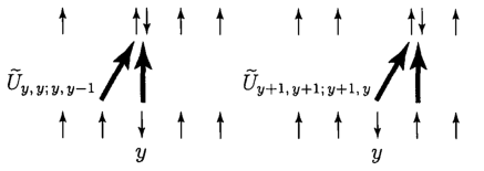
Let us investigate the action of these partial Hamiltonians (2.40)-(2.42) onto the state Ω⁡(k)\Omega(k). It is useful to first consider the action on the state Γy\Gamma_{y} defined in (2.39) which contains a down-spin electron at site yy. By operating the “exchange” Hamiltonian (2.40) onto Γy\Gamma_{y}, we find

H1​Γy\displaystyle H_{1}\Gamma_{y} =\displaystyle= U~y−1,y;y−1,y​(Γy−Γy−1)+U~y,y+1;y,y+1​(Γy−Γy+1)\displaystyle\widetilde{U}_{y-1,y;y-1,y}(\Gamma_{y}-\Gamma_{y-1})+\widetilde{U}_{y,y+1;y,y+1}(\Gamma_{y}-\Gamma_{y+1}) (2.43)
=\displaystyle= U~0,1;0,1​(2​Γy−Γy−1−Γy+1),\displaystyle\widetilde{U}_{0,1;0,1}(2\Gamma_{y}-\Gamma_{y-1}-\Gamma_{y+1}),

where the minus signs come from fermion ordering for the “exchanged” configurations. Figure 4 illustrates how these four terms arise. We also used the translation invariance of U~\widetilde{U}, which is indeed essential for the present proof. Recalling (2.38), we get the expected result

H1​Ω​(k)={E0+4​U~0,1;0,1​(sin⁡k2)2}​Ω​(k).H_{1}\,\Omega(k)=\left\{E_{0}+4\,\widetilde{U}_{0,1;0,1}\left(\sin\frac{k}{2}\right)^{2}\right\}\Omega(k). (2.44)

Refer to caption

Figure 4: When the “exchange” Hamiltonian H1H_{1} acts on the state Γy\Gamma_{y}, four terms are generated. Two of them are the same as Γy\Gamma_{y}, while the electronic spins are exchanged in the other two states. The process illustrated here can be regarded as the ultimate origin of ferromagnetism in the present model.

To see the role of H2H_{2} (2.41), let us operate it onto Γy\Gamma_{y} to get

H2​Γy\displaystyle H_{2}\,\Gamma_{y} =\displaystyle= ∑r=±1{(U~y+r,y+r;y+r,y+τy+r,y)​Γ~y+r(r)−(U~y,y;y,y−r+τy,y−r)​Γ~y(r)}\displaystyle\sum_{r=\pm 1}\left\{(\widetilde{U}_{y+r,y+r;y+r,y}+\tau_{y+r,y})\widetilde{\Gamma}^{(r)}_{y+r}-(\widetilde{U}_{y,y;y,y-r}+\tau_{y,y-r})\widetilde{\Gamma}^{(r)}_{y}\right\} (2.45)
=\displaystyle= (U~r,r;r,0+τr,0)​(Γ~y+r(r)−Γ~y(r)),\displaystyle(\widetilde{U}_{r,r;r,0}+\tau_{r,0})\left(\widetilde{\Gamma}^{(r)}_{y+r}-\widetilde{\Gamma}^{(r)}_{y}\right),

where Γ~y(r)=ay,↓†​by−r,↑​Φ↑\widetilde{\Gamma}^{(r)}_{y}=a^{\dagger}_{y,\downarrow}b_{y-r,\uparrow}\Phi_{\uparrow} is the state with an empty site y−ry-r and a doubly occupied site yy. We also used the translation invariance of U~\widetilde{U} and τ\tau. In Figure 5, we illustrate the action of a part of H2H_{2} onto Γy\Gamma_{y}. Again from (2.38), we find that

H2​Ω​(k)\displaystyle H_{2}\,\Omega(k) =\displaystyle= ∑r=±1e−i​k​r−1α⁡(k)​(U~r,r;r,0+τr,0)​Ξr​(k)\displaystyle\sum_{r=\pm 1}\frac{e^{-ikr}-1}{\alpha(k)}\,(\widetilde{U}_{r,r;r,0}+\tau_{r,0})\,\Xi_{r}(k) (2.46)
=\displaystyle= ∑r=±1e−i​k​r−1α⁡(k)​(U~1,1;1,0+τ1,0)​Ξr​(k),\displaystyle\sum_{r=\pm 1}\frac{e^{-ikr}-1}{\alpha(k)}\,(\widetilde{U}_{1,1;1,0}+\tau_{1,0})\,\Xi_{r}(k),

where we used the reflection symmetry2424 24 Such a symmetry exists in the present model. In the general class of models studied later, we do not assume reflection or rotation symmetries. to get the final line. Here

Ξr​(k)=∑x∈Λoei​k​x​Γ~x(r)=∑x∈Λoei​k​x​ax,↓†​bx−r,↑​Φ↑,\Xi_{r}(k)=\sum_{x\in\Lambda_{o}}e^{ikx}\,\widetilde{\Gamma}^{(r)}_{x}=\sum_{x\in\Lambda_{o}}e^{ikx}\,a^{\dagger}_{x,\downarrow}b_{x-r,\uparrow}\Phi_{\uparrow}, (2.47)

is the state in which a bound pair of an empty site x−rx-r and a doubly occupied site xx is propagating with momentum kk. We shall abbreviate Ξ±1​(k)\Xi_{\pm 1}(k) as Ξ±​(k)\Xi_{\pm}(k).

Refer to caption

Figure 5: When the (effective hopping) operator
∑x∈Λ,σ=↑,↓U~x+1,x+1;x+1,xa†x+1,σa†x+1,−σbx+1,−σbx,σ\sum_{x\in\Lambda,\,\sigma=\uparrow,\downarrow}\widetilde{U}_{x+1,x+1;x+1,x}\,a^{\dagger}_{x+1,\sigma}a^{\dagger}_{x+1,-\sigma}b_{x+1,-\sigma}b_{x,\sigma} acts on Γy\Gamma_{y}, two states with a bound pair of a hole and a doubly occupied site are generated. Note that the two resulting states are related through the translation by a distance 11. This process is the major source of instability against antiferromagnetism.

Similarly we obtain

H3​Ω​(k)=ei​k−1α⁡(k)​U~1/2,1/2;0,1​Θ​(k),H_{3}\,\Omega(k)=\frac{e^{ik}-1}{\alpha(k)}\,\widetilde{U}_{1/2,1/2;0,1}\,\Theta(k), (2.48)

where

Θ⁡(k)=∑x∈Λoei​k​x​ax+(1/2),↓†​ax+(1/2),↑†​bx,↑​bx+1,↑​Φ↑,\Theta(k)=\sum_{x\in\Lambda_{o}}e^{ikx}\,a^{\dagger}_{x+(1/2),\downarrow}a^{\dagger}_{x+(1/2),\uparrow}b_{x,\uparrow}b_{x+1,\uparrow}\Phi_{\uparrow}, (2.49)

is the state in which two adjacent empty sites in Λo\Lambda_{o} and a doubly occupied site in between them are forming a bound state and propagating with momentum kk. See Figure 6 for schematic pictures of the states2525 25 In the general notation used in the latter sections, the states Ξr​(k)\Xi_{r}(k) and Θ⁡(k)\Theta(k) are denoted as Φ0,r​(k)\Phi_{0,r}(k) and Φ1/2,1/2,0,1​(k)\Phi_{1/2,1/2,0,1}(k), respectively. See Section 6.2. Ω⁡(k)\Omega(k), Ξ+​(k)\Xi_{+}(k), and Θ⁡(k)\Theta(k). We also note here that these states all belong to the Hilbert space ℋk{\cal H}_{k}, which we introduced just above Theorem 2.4.

The relations (2.46) and (2.48) clearly show that our trial state Ω⁡(k)\Omega(k) cannot be the exact eigenstate of the Hamiltonian. To investigate low-lying spectrum of HH, we have to consider (at least) the subspace spanned by the states Ω⁡(k)\Omega(k), Ξ±​(k)\Xi_{\pm}(k), and Θ⁡(k)\Theta(k). As before we calculate the action of HH onto the latter states to find

H​Ξ±​(k)\displaystyle H\,\Xi_{\pm}(k) ≃\displaystyle\simeq (E0+U~0,0;0,0)​Ξ±​(k)+α⁡(k)​(U~0,1;1,1+τ0,1)​(e∓i​k−1)​Ω​(k)\displaystyle(E_{0}+\widetilde{U}_{0,0;0,0})\,\Xi_{\pm}(k)+\alpha(k)\,(\widetilde{U}_{0,1;1,1}+\tau_{0,1})(e^{\mp ik}-1)\,\Omega(k) (2.50)
+(other states),\displaystyle+(\mbox{other states}),

and

H​Θ​(k)\displaystyle H\Theta(k) ≃\displaystyle\simeq (E0−2​τ0,0+2​τ1/2,1/2+U~1/2,1/2;1/2,1/2)​Θ​(k)\displaystyle(E_{0}-2\,\tau_{0,0}+2\,\tau_{1/2,1/2}+\widetilde{U}_{1/2,1/2;1/2,1/2})\Theta(k) (2.51)
+α⁡(k)​(e−i​k−1)​U~0,1;1/2,1/2​Ω​(k)+(other states).\displaystyle+\alpha(k)(e^{-ik}-1)\widetilde{U}_{0,1;1/2,1/2}\,\Omega(k)+(\mbox{other states}).

Although it might not be clear at this stage, it turns out that the “other states” in (2.50) and (2.51) do not play essential roles. We leave such estimates (as well as the precise definition of the “other states”) to the latter sections, and simply neglect them here.

The equations (2.44), (2.46), (2.48), (2.50), and (2.51) provide, for each k∈𝒦k\in{\cal K}, the representation of the Hamiltonian in the four dimensional subspace of ℋk{\cal H}_{k} spanned by the states Ω⁡(k)\Omega(k), Ξ±​(k)\Xi_{\pm}(k), and Θ⁡(k)\Theta(k). We now read off the matrix elements2626 26 As usual, matrix elements h⁡[Ψ,Φ]h[\Psi,\Phi] are defined by the unique expansion H​Φ=∑Ψh⁡[Ψ,Φ]​ΨH\Phi=\sum_{\Psi}h[\Psi,\Phi]\Psi. See also (6.2). from these equations, and then use the estimates (2.26)-(2.30) of U~\widetilde{U} to evaluate them as

h⁡[Ω⁡(k),Ω⁡(k)]≃E0+4​U~0,1;0,1​(sin⁡k2)2≃E0+4​Uλ4​(sin⁡k2)2,h[\Omega(k),\Omega(k)]\simeq E_{0}+4\,\widetilde{U}_{0,1;0,1}\left(\sin\frac{k}{2}\right)^{2}\\ \simeq E_{0}+4\frac{U}{\lambda^{4}}\left(\sin\frac{k}{2}\right)^{2},
h⁡[Ξ±​(k),Ξ±​(k)]≃E0+U~0,0;0,0≃E0+U,h[\Xi_{\pm}(k),\Xi_{\pm}(k)]\simeq E_{0}+\widetilde{U}_{0,0;0,0}\simeq E_{0}+U, (2.52)
h⁡[Θ⁡(k),Θ⁡(k)]≃E0−2​τ0,0+2​τ1/2,1/2+U~1/2,1/2;1/2,1/2≃E0+2​λ2​t+U,h[\Theta(k),\Theta(k)]\simeq E_{0}-2\,\tau_{0,0}+2\,\tau_{1/2,1/2}+\widetilde{U}_{1/2,1/2;1/2,1/2}\\ \simeq E_{0}+2\lambda^{2}t+U,
h⁡[Ξ±​(k),Ω⁡(k)]\displaystyle h[\Xi_{\pm}(k),\Omega(k)] ≃\displaystyle\simeq α​(k)−1​(U~1,1;1,0+τ1,0)​(e±i​k−1)\displaystyle\alpha(k)^{-1}(\widetilde{U}_{1,1;1,0}+\tau_{1,0})(e^{\pm ik}-1) (2.53)
≃\displaystyle\simeq α​(k)−1​(c​U​ρλ2+Uλ4+c′​ρ​t)​(e±i​k−1),\displaystyle\alpha(k)^{-1}\left(\frac{cU\rho}{\lambda^{2}}+\frac{U}{\lambda^{4}}+c^{\prime}\rho t\right)(e^{\pm ik}-1),
h⁡[Ω⁡(k),Ξ±​(k)]\displaystyle h[\Omega(k),\Xi_{\pm}(k)] ≃\displaystyle\simeq α⁡(k)​(U~0,1;1,1+τ0,1)​(e∓i​k−1)\displaystyle\alpha(k)(\widetilde{U}_{0,1;1,1}+\tau_{0,1})(e^{\mp ik}-1) (2.54)
≃\displaystyle\simeq α⁡(k)​(−Uλ2+c′​ρ​t)​(e∓i​k−1),\displaystyle\alpha(k)\left(-\frac{U}{\lambda^{2}}+c^{\prime}\rho t\right)(e^{\mp ik}-1),
h⁡[Θ⁡(k),Ω⁡(k)]≃α​(k)−1​U~1/2,1/2;0,1​(ei​k−1)≃α​(k)−1​Uλ2​(ei​k−1),h[\Theta(k),\Omega(k)]\simeq\alpha(k)^{-1}\,\widetilde{U}_{1/2,1/2;0,1}(e^{ik}-1)\simeq\alpha(k)^{-1}\frac{U}{\lambda^{2}}(e^{ik}-1), (2.55)

and

h⁡[Θ⁡(k),Ω⁡(k)]≃α⁡(k)​U~0,1;1/2,1/2​(e−i​k−1)≃α⁡(k)​Uλ2​(e−i​k−1),h[\Theta(k),\Omega(k)]\simeq\alpha(k)\,\widetilde{U}_{0,1;1/2,1/2}(e^{-ik}-1)\simeq\alpha(k)\frac{U}{\lambda^{2}}(e^{-ik}-1), (2.56)

where the approximate values are obtained for λ≫1\lambda\gg 1 and |ρ|/λ2≪1\left|\rho\right|/\lambda^{2}\ll 1, and cc, c′c^{\prime} are constants. Reflecting the use of the non-orthonormal basis, these matrix elements are not symmetric. In particular drastic difference between the elements h⁡[Ξ±​(k),Ω⁡(k)]h[\Xi_{\pm}(k),\Omega(k)] (2.53) and h⁡[Ω⁡(k),Ξ±​(k)]h[\Omega(k),\Xi_{\pm}(k)] (2.54) plays fundamental role in our proof. Figure 6 shows these matrix elements.

Refer to caption

Figure 6: Schematic pictures of the states Ω⁡(k)\Omega(k), Ξ+​(k)\Xi_{+}(k), and Θ⁡(k)\Theta(k), and the matrix elements between them. As for the off-diagonal matrix elements, we only present the main part of their absolute values. Note that the matrix elements between Ω⁡(k)\Omega(k) and Ξ+​(k)\Xi_{+}(k) are highly asymmetric (apart from the artificial asymmetry factor α⁡(k)\alpha(k)). The small out-going matrix elements from Ω⁡(k)\Omega(k) indicates that the state Ω⁡(k)\Omega(k) is a good trial state for the spin-wave excitation.

In order to bound the excitation energy from below, we use the following wellknown fact about the minimum eigenvalue of a matrix. Let (hi,j)i,j=1,…,N(h_{i,j})_{i,j=1,\ldots,N} be an N×NN\times N matrix with real eigenvalues. Then the lowest eigenvalue h0h_{0} of the matrix satisfies h0≥mini=1,…,N⁡Dih_{0}\geq\min_{i=1,\ldots,N}D_{i} with Di=Re⁡[hi,i]−∑j≠i|hi,j|D_{i}={\rm Re}[h_{i,i}]-\sum_{j\neq i}|h_{i,j}|. This is almost trivial, but see Lemma 6.4 for a proof. We stress that this simple-minded inequality is expected to yield physically meaningful results only when one uses a basis which “almost diagonalizes” the low energy part of the Hamiltonian.

We now apply this inequality to the 4×44\times 4 matrix representation of HH in each sector with a fixed k∈𝒦k\in{\cal K}. The quantities corresponding to DiD_{i} are evaluated for each state as

D⁡[Ω⁡(k)]=h⁡[Ω⁡(k),Ω⁡(k)]−∑±|h⁡[Ω⁡(k),Ξ±​(k)]|−|h⁡[Ω⁡(k),Θ⁡(k)]|\displaystyle D[\Omega(k)]=h[\Omega(k),\Omega(k)]-\sum_{\pm}\left|h[\Omega(k),\Xi_{\pm}(k)]\right|-\left|h[\Omega(k),\Theta(k)]\right|
≥E0+4​Uλ4​(sin⁡k2)2−4​α​(k)​(Uλ2+c′​|ρ|​t)​|sin⁡k2|−2​α​(k)​Uλ2​|sin⁡k2|,\displaystyle\geq E_{0}+\frac{4U}{\lambda^{4}}\left(\sin\frac{k}{2}\right)^{2}-4\alpha(k)\left(\frac{U}{\lambda^{2}}+c^{\prime}\left|\rho\right|t\right)\left|\sin\frac{k}{2}\right|-2\alpha(k)\frac{U}{\lambda^{2}}\left|\sin\frac{k}{2}\right|, (2.57)
D​[Ξ±​(k)]\displaystyle D[\Xi_{\pm}(k)] =\displaystyle= h⁡[Ξ±​(k),Ξ±​(k)]−|h⁡[Ξ±​(k),Ω⁡(k)]|\displaystyle h[\Xi_{\pm}(k),\Xi_{\pm}(k)]-\left|h[\Xi_{\pm}(k),\Omega(k)]\right| (2.58)
≥\displaystyle\geq E0+U−2​α​(k)−1​(c​U​|ρ|λ2+Uλ4+c′​|ρ|​t)​|sin⁡k2|,\displaystyle E_{0}+U-2\alpha(k)^{-1}\left(\frac{cU\left|\rho\right|}{\lambda^{2}}+\frac{U}{\lambda^{4}}+c^{\prime}\left|\rho\right|t\right)\left|\sin\frac{k}{2}\right|,

and

D⁡[Θ⁡(k)]\displaystyle D[\Theta(k)] =\displaystyle= h⁡[Θ⁡(k),Θ⁡(k)]−|h⁡[Θ⁡(k),Ω⁡(k)]|\displaystyle h[\Theta(k),\Theta(k)]-\left|h[\Theta(k),\Omega(k)]\right| (2.59)
≥\displaystyle\geq E0+2​λ2​t+U−2​α​(k)−1​Uλ2​|sin⁡k2|,\displaystyle E_{0}+2\lambda^{2}t+U-2\alpha(k)^{-1}\frac{U}{\lambda^{2}}\left|\sin\frac{k}{2}\right|,

where we used the estimates (2.7)-(2.56) to get the lower bounds.

At this stage, we choose2727 27 The choice of α⁡(k)\alpha(k) here is different from that in the full proof in Section 6. (See (6.31).) This is because the actual estimate of D​[Ξ±​(k)]D[\Xi_{\pm}(k)] in the latter sections take into account various small terms which are simply neglected here. the constant α⁡(k)\alpha(k) as

α⁡(k)=4​(c​|ρ|λ2+1λ4+c′​|ρ|​tU)​|sin⁡k2|.\alpha(k)=4\left(\frac{c\left|\rho\right|}{\lambda^{2}}+\frac{1}{\lambda^{4}}+\frac{c^{\prime}\left|\rho\right|t}{U}\right)\left|\sin\frac{k}{2}\right|. (2.60)

This choice makes the bound (2.58) into

D⁡[Ξ±​(k)]≥E0+U2,D[\Xi_{\pm}(k)]\geq E_{0}+\frac{U}{2}, (2.61)

and the bound (2.59) into

D⁡[Θ⁡(k)]\displaystyle D[\Theta(k)] ≥\displaystyle\geq E0+2​λ2​t+U−U2​λ2​(c​|ρ|λ2+1λ4+c′​|ρ|​tU)−1\displaystyle E_{0}+2\lambda^{2}t+U-\frac{U}{2\lambda^{2}}\left(\frac{c\left|\rho\right|}{\lambda^{2}}+\frac{1}{\lambda^{4}}+\frac{c^{\prime}\left|\rho\right|t}{U}\right)^{-1} (2.62)
≥\displaystyle\geq E0+2​λ2​t+U−λ2​U2\displaystyle E_{0}+2\lambda^{2}t+U-\frac{\lambda^{2}U}{2}
≥\displaystyle\geq E0+U,\displaystyle E_{0}+U,

where we have further assumed2828 28 The upper bound required for UU depends sensitively on the choice of α⁡(k)\alpha(k). The requirement U≤K2​λ​tU\leq K_{2}\lambda t made in Theorem 2.4 (and which appears in the full proof) is somewhat different from the present one. U≤4​tU\leq 4t. Finally we substitute (2.60) into the bound (2.57) to get

D⁡[Ω⁡(k)]\displaystyle D[\Omega(k)] ≥\displaystyle\geq E0+4​Uλ4​(sin⁡k2)2\displaystyle E_{0}+\frac{4U}{\lambda^{4}}\left(\sin\frac{k}{2}\right)^{2} (2.63)
−4​(c​|ρ|λ2+1λ4+c′​|ρ|​tU)​(6​Uλ2+4​c′​|ρ|​t)​(sin⁡k2)2\displaystyle-4\left(\frac{c\left|\rho\right|}{\lambda^{2}}+\frac{1}{\lambda^{4}}+\frac{c^{\prime}\left|\rho\right|t}{U}\right)\left(\frac{6U}{\lambda^{2}}+4c^{\prime}\left|\rho\right|t\right)\left(\sin\frac{k}{2}\right)^{2}
=\displaystyle= E0+4​Uλ4​{1−(c​|ρ|+1λ2+c′​|ρ|​λ2​tU)​(6+4​c′​|ρ|​λ2​tU)}​(sin⁡k2)2\displaystyle E_{0}+\frac{4U}{\lambda^{4}}\left\{1-\left(c\left|\rho\right|+\frac{1}{\lambda^{2}}+\frac{c^{\prime}\left|\rho\right|\lambda^{2}t}{U}\right)\left(6+\frac{4c^{\prime}\left|\rho\right|\lambda^{2}t}{U}\right)\right\}\left(\sin\frac{k}{2}\right)^{2}
≥\displaystyle\geq E0+4​Uλ4​{1−A1​|ρ|−A2λ−A3​λ2​t​|ρ|U}​(sin⁡k2)2,\displaystyle E_{0}+\frac{4U}{\lambda^{4}}\left\{1-A_{1}\left|\rho\right|-\frac{A_{2}}{\lambda}-\frac{A_{3}\lambda^{2}t\left|\rho\right|}{U}\right\}\left(\sin\frac{k}{2}\right)^{2},

with constants2929 29 Here the term A2/λA_{2}/\lambda in the right-hand side of (2.63) can be replaced with A2/λ2A_{2}/\lambda^{2} if we simply equate the above expression. Since the actual matrix elements have many “small” terms that are neglected here, what we can prove (in the latter sections with perfect rigor) is the bound in terms of the quantity in the right-hand side of (2.63). A1A_{1}, A2A_{2}, and A3A_{3}. Since the lower bounds (2.58) and (2.59) for D​[Ξ±​(k)]D[\Xi_{\pm}(k)] and D⁡[Θ⁡(k)]D[\Theta(k)] are strictly larger than that for D⁡[Ω⁡(k)]D[\Omega(k)], we find that the right-hand side of (2.63) gives the desired lower bound for the lowest eigenvalue of the Hamiltonian in the space ℋk{\cal H}_{k}. Therefore the lower bound for the spin wave excitation in (2.10) (which is the main statement of Theorem 2.4) has been derived.

In the remainder, we sketch how we get Theorem 2.9 about the local stability of ferromagnetism from the above lower bounds. The lower bounds in (2.10) gives strict bounds ESW​(k)>E0E_{\rm SW}(k)>E_{0} for all k∈𝒦k\in{\cal K} except for k=0k=0. This means that the desired local stability inequality (2.9) has been proved except in the translation invariant sector with k=0k=0. To deal with the k=0k=0 sector is easy once we realize that Ω⁡(0)\Omega(0) is nothing but an S​U​(2)SU(2) rotation of the “ferromagnetic ground state” Φ↑\Phi_{\uparrow}. By simply repeating the above arguments for the three dimensional subspace spanned by Ξ±​(0)\Xi_{\pm}(0) and Θ⁡(0)\Theta(0), we easily find that the desired bound (2.9) also holds in the sector with k=0k=0. It only remains to extend the parameter region in which the statement is valid. This is easily done by a general consideration about the monotonicity of energies as a function of UU. See Section 6.4.

3 Definitions and Main Results

In the present section, we define the general class of models treated in the present paper, and precisely state our main theorems.

3.1 Lattice

We describe the lattice on which our Hubbard model is defined. The lattice is characterized by the dimension of the lattice d=1,2,3,⋯d=1,2,3,\cdots, the dimension of “cells” ν=1,2,⋯,d\nu=1,2,\cdots,d, and the linear size LL which is taken to be an odd integer. Throughout the present paper we assume that the three parameters dd, ν\nu, and LL are fixed to allowed values. All the bounds proved in the present paper are independent of the system size LL.

Let Λo\Lambda_{o} be the dd-dimensional L×…×LL\times\ldots\times L hypercubic lattice with periodic boundary conditions;

Λo={x=(x1,…,xd)|xi∈𝐙, |xi|≤(L−1)/2 for i=1,…,d}.\Lambda_{o}=\left\{x=(x_{1},\ldots,x_{d})\,\Bigl|\,\mbox{$x_{i}\in{\bf Z}$, $\left|x_{i}\right|\leq(L-1)/2$ for $i=1,\ldots,d$}\right\}. (3.1)

We “decorate” the lattice Λo\Lambda_{o} by adding sites taken at the center of each ν\nu-dimensional cell. Let 𝒰′{\cal U}^{\prime} be the set of vectors defined as

𝒰′={u=(u1,…,ud)|ui=0 or 1/2, and 2​∑i=1dui=ν}.{\cal U}^{\prime}=\left\{u=(u_{1},\ldots,u_{d})\,\Bigl|\,\mbox{$u_{i}=0$ or $1/2$, and $2\sum_{i=1}^{d}u_{i}=\nu$}\right\}. (3.2)

Note that each u∈𝒰′u\in{\cal U}^{\prime} has the length |u|=ν/2\left|u\right|=\sqrt{\nu}/2. For each u∈𝒰′u\in{\cal U}^{\prime}, we let

Λu={x+u|x∈Λo}.\Lambda_{u}=\left\{x+u\,\Bigl|\,x\in\Lambda_{o}\right\}. (3.3)

By introducing the unit cell 𝒰{\cal U} of the lattice by

𝒰={o}∪𝒰′,{\cal U}=\left\{o\right\}\cup{\cal U}^{\prime}, (3.4)

where o=(0,⋯,0)o=(0,\cdots,0), our decorated hypercubic lattice is defined as

Λ=⋃u∈𝒰Λu.\Lambda=\bigcup_{u\in{\cal U}}\Lambda_{u}. (3.5)

We often decompose Λ\Lambda as Λ=Λo∪Λ′\Lambda=\Lambda_{o}\cup\Lambda^{\prime} where

Λ′=⋃u∈𝒰′Λu.\Lambda^{\prime}=\bigcup_{u\in{\cal U}^{\prime}}\Lambda_{u}. (3.6)

As is discussed in Section 2.1, we can imagine that sites in Λo\Lambda_{o} represent metallic atoms and sites in Λ′\Lambda^{\prime} represent oxygen atoms. The numbers of sites (vectors) in the unit cell3030 30 Throughout the present paper, |S|\left|S\right| denotes the number of elements in a set SS.

b=|𝒰|=(dν)+1b=\left|{\cal U}\right|={d\choose\nu}+1 (3.7)

is important, since it gives the number of the bands in the corresponding single-electron problem.

For d=1d=1, the only possible choice of ν\nu is ν=1\nu=1, and we get the chain with two kinds of atoms discussed in Section 2. (See Figure 1.) For d=2d=2, we can either set ν=1\nu=1 to get the lattice in Figure 7a with the band number b=3b=3, or set ν=2\nu=2 to get the lattice in Figure 7b with b=2b=2. For d=3d=3, there are three choices for ν\nu. The lattices with ν=2\nu=2 and ν=3\nu=3 have the structures similar to the fcc and the bcc lattices, respectively.

Refer to caption

Figure 7: The lattice Λ\Lambda in two dimensions (d=2d=2) with a) ν=1\nu=1, and b) ν=2\nu=2. The black dots are sites in Λo\Lambda_{o} and the gray dots are sites in Λ′\Lambda^{\prime}. One may interpret black sits as metallic atoms and gray sites as oxygen atoms.

We introduce some sets of lattice vectors which will become useful. We define

ℱo={f=(f1,…,fd)|fi=0 or ±1/2, and 2​∑i=1d|fi|=ν},{\cal F}_{o}=\left\{f=(f_{1},\ldots,f_{d})\,\Bigl|\,\mbox{$f_{i}=0$ or $\pm 1/2$, and $2\sum_{i=1}^{d}|f_{i}|=\nu$}\right\}, (3.8)

which is the collection of the sites in Λ′\Lambda^{\prime} adjacent to the origin oo. We have |ℱo|=2ν​(dν)\left|{\cal F}_{o}\right|=2^{\nu}{d\choose\nu}. For f∈ℱof\in{\cal F}_{o}, we define

ℱf={g∈ℱo||gi|=|fi| for i=1,…,d}.{\cal F}_{f}=\left\{g\in{\cal F}_{o}\,\Bigl|\,\mbox{$\left|g_{i}\right|=\left|f_{i}\right|$ for $i=1,\ldots,d$}\right\}. (3.9)

Note that for a fixed f∈ℱof\in{\cal F}_{o}, {f+g|g∈ℱf}\left\{f+g\,\Bigl|\,g\in{\cal F}_{f}\right\} is the set of sites in Λo\Lambda_{o} which are adjacent to ff. We have |ℱf|=2ν\left|{\cal F}_{f}\right|=2^{\nu}. We also note that for g∈ℱfg\in{\cal F}_{f}, we have

ℱg=ℱf.{\cal F}_{g}={\cal F}_{f}. (3.10)

3.2 Hubbard Model

We define the Hubbard model on the decorated hypercubic lattice Λ\Lambda. As usual, we denote by cx,σ†c^{\dagger}_{x,\sigma} and cx,σc_{x,\sigma} the creation and the annihilation operators, respectively, of an electron at site x∈Λx\in\Lambda with spin σ=↑\sigma=\uparrow, ↓\downarrow. These operators satisfy the standard anticommutation relations

{cx,σ,cy,τ}={cx,σ†,cy,τ†}=0,\left\{c_{x,\sigma},c_{y,\tau}\right\}=\left\{c^{\dagger}_{x,\sigma},c^{\dagger}_{y,\tau}\right\}=0, (3.11)

and

{cx,σ,cy,τ†}=δx,y​δσ,τ,\left\{c_{x,\sigma},c^{\dagger}_{y,\tau}\right\}=\delta_{x,y}\,\delta_{\sigma,\tau}, (3.12)

for any x,y∈Λx,y\in\Lambda and σ,τ=↑,↓\sigma,\tau=\uparrow,\downarrow, where {A,B}=A​B+B​A\left\{A,B\right\}=AB+BA. The number operator for an electron at site xx with spin σ\sigma is defined as

nx,σ=cx,σ†​cx,σ.n_{x,\sigma}=c^{\dagger}_{x,\sigma}c_{x,\sigma}. (3.13)

We consider the standard Hubbard Hamiltonian

H=Hhop+Hint.H=H_{\rm hop}+H_{\rm int}. (3.14)

The interaction Hamiltonian is

Hint=U​∑x∈Λnx,↑​nx,↓,H_{\rm int}=U\sum_{x\in\Lambda}n_{x,\uparrow}n_{x,\downarrow}, (3.15)

where U>0U>0 is the on-site Coulomb repulsion energy. The hopping Hamiltonian is further decomposed as

Hhop=Hhop(0)+ρ​Hhop′,H_{\rm hop}=H_{\rm hop}^{(0)}+\rho H^{\prime}_{\rm hop}, (3.16)

where Hhop(0)H_{\rm hop}^{(0)} is the hopping Hamiltonian of the flat-band model defined as

Hhop(0)=t​∑σ=↑,↓∑x∈Λ′(λ​cx,σ†+∑y∈Λo|x−y|=ν/2cy,σ†)​(λ​cx,σ+∑y∈Λo|x−y|=ν/2cy,σ),H_{\rm hop}^{(0)}=t\sum_{\sigma=\uparrow,\downarrow}\sum_{x\in\Lambda^{\prime}}\left(\lambda\,c^{\dagger}_{x,\sigma}+\mathop{\sum_{y\in\Lambda_{o}}}_{|x-y|=\sqrt{\nu}/2}c^{\dagger}_{y,\sigma}\right)\left(\lambda\,c_{x,\sigma}+\mathop{\sum_{y\in\Lambda_{o}}}_{|x-y|=\sqrt{\nu}/2}c_{y,\sigma}\right), (3.17)

where t>0t>0 and λ>0\lambda>0 are parameters. It is, of course, possible to represent the Hamiltonian in the “standard” form as

Hhop(0)=∑σ=↑,↓∑x,y∈Λtx,y(0)​cx,σ†​cy,σ,H_{\rm hop}^{(0)}=\sum_{\sigma=\uparrow,\downarrow}\sum_{x,y\in\Lambda}t_{x,y}^{(0)}\,c^{\dagger}_{x,\sigma}c_{y,\sigma}, (3.18)

where the hopping matrix elements are given by

tx,y(0)=ty,x(0)={λ2​tif x=y∈Λ′;λ​tif x∈Λo, y∈Λ′ with |x−y|=ν/2;2(ν−μ)​(d−μν−μ)​tif x,y∈Λo with |x−y|=μ where μ=0,1,…,ν;0otherwise.t_{x,y}^{(0)}=t_{y,x}^{(0)}=\cases{\lambda^{2}t&if $x=y\in\Lambda^{\prime}$;\cr\lambda t&if $x\in\Lambda_{o}$, $y\in\Lambda^{\prime}$ with $\left|x-y\right|=\sqrt{\nu}/2$;\cr 2^{(\nu-\mu)}{d-\mu\choose\nu-\mu}t&if $x,y\in\Lambda_{o}$ with $\left|x-y\right|=\sqrt{\mu}$ where $\mu=0,1,\ldots,\nu$;\cr 0&otherwise.\cr} (3.19)

The representation (3.17) shows that the hopping Hamiltonian Hhop(0)H_{\rm hop}^{(0)} is characterized by mean-field-like hoppings within each ν\nu-dimensional cell which consists of x∈Λ′x\in\Lambda^{\prime} and the sites y∈Λoy\in\Lambda_{o} adjacent to it. This rather artificial choice of the hopping produces the single-electron spectrum with a completely flat band. See Section 4.1.

The perturbation Hamiltonian, on the other hand, is rather arbitrary. The magnitude of the perturbation is controlled by the real parameter ρ\rho. The Hamiltonian Hhop′H^{\prime}_{\rm hop} has the standard form

Hhop′=∑σ=↑,↓∑x,y∈Λtx,y′​cx,σ†​cy,σ.H^{\prime}_{\rm hop}=\sum_{\sigma=\uparrow,\downarrow}\sum_{x,y\in\Lambda}t^{\prime}_{x,y}\,c^{\dagger}_{x,\sigma}c_{y,\sigma}. (3.20)

The hopping matrix elements tx,y′=ty,x′∈𝐑t^{\prime}_{x,y}=t^{\prime}_{y,x}\in{\bf R} are arbitrary except for the following conditions. We require the translation invariance

tx,y′=tx+z,y+z′t^{\prime}_{x,y}=t^{\prime}_{x+z,y+z} (3.21)

for any z∈𝐙dz\in{\bf Z}^{d} and any x,y∈Λx,y\in\Lambda, and the summability

∑y∈Λ|tx,y′|≤t,\sum_{y\in\Lambda}\left|t^{\prime}_{x,y}\right|\leq t, (3.22)
∑y∈Λ|x−y|​|tx,y′|≤t​R,\sum_{y\in\Lambda}\left|x-y\right|\left|t^{\prime}_{x,y}\right|\leq t\,R, (3.23)

for any x∈Λx\in\Lambda. Here tt is the same as before, and RR is a constant which measures the range of the hopping {tx,y′}\left\{t^{\prime}_{x,y}\right\}. When RR chosen to optimize (3.23) is less than ν/2\sqrt{\nu}/2, we redefine it3131 31 This is done for a purely technical reason to make some formulas simple. See (10.90). as R=ν/2R=\sqrt{\nu}/2.

The Hilbert space of the model is spanned by the basis states

ΦA,B=(∏y∈Acy,↑†)​(∏z∈Bcz,↓†)​Φvac,\Phi_{A,B}=\left(\prod_{y\in A}c^{\dagger}_{y,\uparrow}\right)\left(\prod_{z\in B}c^{\dagger}_{z,\downarrow}\right)\Phi_{\rm vac}, (3.24)

where AA, BB are subsets of Λ\Lambda, and Φvac\Phi_{\rm vac} is the unique vacuum state characterized by cx,σ​Φvac=0c_{x,\sigma}\Phi_{\rm vac}=0 for any x∈Λx\in\Lambda and σ=↑,↓\sigma=\uparrow,\downarrow. In the preset work, we only consider the Hilbert space ℋ{\cal H} with the electron number fixed to Ld=|Λo|L^{d}=\left|\Lambda_{o}\right|, which is spanned by the basis states (3.24) with |A|+|B|=Ld\left|A\right|+\left|B\right|=L^{d}.

3.3 Local Stability Theorem

The total spin operator of the Hubbard model is defined as usual by

Stot(α)=12​∑x∈Λ∑σ,τ=↑,↓cx,σ†​(p(α))σ,τ​cx,τS^{(\alpha)}_{\rm tot}=\frac{1}{2}\sum_{x\in\Lambda}\sum_{\sigma,\tau=\uparrow,\downarrow}c^{\dagger}_{x,\sigma}(p^{(\alpha)})_{\sigma,\tau}\,c_{x,\tau} (3.25)

for α=1,2,3\alpha=1,2,3, where p(α)p^{(\alpha)} are the Pauli matrices

p(1)=(0110),p(2)=(0−ii0),p(3)=(100−1).p^{(1)}=\left(\matrix{0&1\cr 1&0\cr}\right),\quad p^{(2)}=\left(\matrix{0&-i\cr i&0\cr}\right),\quad p^{(3)}=\left(\matrix{1&0\cr 0&-1\cr}\right). (3.26)

An explicit calculation shows that the spin operators (𝐒tot)2=∑α=1,2,3(Stot(α))2({\bf S}_{\rm tot})^{2}=\sum_{\alpha=1,2,3}(S^{(\alpha)}_{\rm tot})^{2}, Stot(3)S_{\rm tot}^{(3)}, and the Hamiltonian HH commute with each other. This means that we can find simultaneous eigenstates of these operators. The eigenvalue of (𝐒tot)2({\bf S}_{\rm tot})^{2} is denoted as Stot​(Stot+1)S_{\rm tot}(S_{\rm tot}+1) where StotS_{\rm tot} can take values 1/2,3/2,…,Smax1/2,3/2,\ldots,S_{\rm max} with Smax=Ld/2S_{\rm max}=L^{d}/2.

We are now able to state the theorem due to Tasaki [47] and Mielke-Tasaki [34].

Theorem 3.1 (Flat-band ferromagnetism)

Consider the Hubbard model with the Hamiltonian (3.14). Assume t>0t>0, λ>0\lambda>0, and ρ=0\rho=0 to get a model with a flat band. Then, for any U>0U>0, the ground states of the Hamiltonian HH has Stot=SmaxS_{\rm tot}=S_{\rm max}, and are non-degenerate apart from the trivial (2​Smax+1)(2S_{\rm max}+1)-fold spin degeneracy.

This theorem is desirable in the sense that it completely determines the ground states of the model. But the result is not robust since it applies only to the models with a completely flat band. Since the references [47, 34] only discusses the models with ν=1\nu=1, we will prove the theorem in Section 5.4.

We now describe the new robust results for the models with a nearly flat band. For Stot=1/2,3/2,…,SmaxS_{\rm tot}=1/2,3/2,\ldots,S_{\rm max}, we denote by Emin​(Stot)E_{\rm min}(S_{\rm tot}) the lowest eigenvalue of the Hamiltonian (3.14) in the sector which consists of the states Φ\Phi such that (𝐒tot)2​Φ=Stot​(Stot+1)​Φ({\bf S}_{\rm tot})^{2}\Phi=S_{\rm tot}(S_{\rm tot}+1)\Phi. Then we have the following simple lemma for the sector with Stot=SmaxS_{\rm tot}=S_{\rm max}.

Lemma 3.2 (“Ferromagnetic ground states”)

Assume that t>0t>0, λ≥λ1\lambda\geq\lambda_{1}, and
|ρ|​λ−2≤r1|\rho|\lambda^{-2}\leq r_{1}, where λ1\lambda_{1} and r1r_{1} are finite constants which depend only on the dimensions dd and ν\nu. (See Lemma 4.1 for explicit formulas of λ1\lambda_{1} and r1r_{1}.) Then for arbitrary UU, the states Φ\Phi such that (𝐒tot)2​Φ=Smax​(Smax+1)​Φ({\bf S}_{\rm tot})^{2}\Phi=S_{\rm max}(S_{\rm max}+1)\Phi and H​Φ=Emin​(Smax)​ΦH\Phi=E_{\rm min}(S_{\rm max})\Phi are non-degenerate apart from the trivial (2​Smax+1)(2S_{\rm max}+1)-fold spin degeneracy.

This lemma is almost trivial, but will be proved in Section 5.3. For convenience, we call the state Φ\Phi characterized by the above lemma the “ferromagnetic ground states”. These states are the energy minimizers in the sector with Stot=SmaxS_{\rm tot}=S_{\rm max}, and are not necessarily the true ground states. We shall remind the readers about this abuse of terminology by always putting the “ferromagnetic ground states” into quotation marks.

The first theorem establishes the instability of the “ferromagnetic ground states” against a single-spin flip. Let ε¯\bar{\varepsilon} denote the band width of the lowest band. (See Section 4.1.) For ρ≠0\rho\neq 0 and a generic choice of {tx,y′}\left\{t^{\prime}_{x,y}\right\}, the band width ε¯\bar{\varepsilon} is strictly positive.

Theorem 3.3 (Instability of the “ferromagnetic ground states”)

Assume the conditions for Lemma 3.2. We also assume that ε¯>0\bar{\varepsilon}>0 (which is generically true if ρ≠0\rho\neq 0), and

0≤U<ε¯.0\leq U<\bar{\varepsilon}. (3.27)

Then the “ferromagnetic ground states” are unstable under a single-spin flip in the sense that

Emin​(Smax−1)<Emin​(Smax).E_{\rm min}(S_{\rm max}-1)<E_{\rm min}(S_{\rm max}). (3.28)

The theorem will be proved in Section 5.3.

Theorem 3.28 shows that one can lower the energy by flipping a single spin in the “ferromagnetic ground states”. It only shows that the “ferromagnetic ground states” are not the true ground states. To identify the true ground states (for U≠0U\neq 0) in this situation is a highly nontrivial and interesting question.

To show the instability of a certain state (as in the above theorem) is not a hard task since one can rely on the standard variational argument. A really important (and difficult) part of the present work is to show the following theorem which states the stability.

Theorem 3.4 (Local stability of the “ferromagnetic ground states”)

Consider the Hubbard model with the Hamiltonian (3.14). Assume that the parameters satisfy

λ≥λ2,|ρ|≤ρ1,λ​|ρ|≤p1\lambda\geq\lambda_{2},\quad\left|\rho\right|\leq\rho_{1},\quad\lambda\left|\rho\right|\leq p_{1} (3.29)

and

U≥K1​λ2​t​|ρ|,U\geq K_{1}\lambda^{2}t\left|\rho\right|, (3.30)

where λ2\lambda_{2}, ρ1\rho_{1}, p1p_{1}, and K1K_{1} are positive constants which depend only on the basic parameters dd, ν\nu, and RR. Then the “ferromagnetic ground states” are stable under a single-spin flip in the sense that

Emin​(Smax−1)>Emin​(Smax).E_{\rm min}(S_{\rm max}-1)>E_{\rm min}(S_{\rm max}). (3.31)

We stress that the problem of stability against a single-spin flip is already a highly nontrivial many-body problem. The restriction to the sector with Stot=Smax−1S_{\rm tot}=S_{\rm max}-1 does not reduce the problem to that of a single-particle (such as a magnon) since there are plenty of spaces for the electrons to move around. Moreover there is no way of expressing the eigenstates as Slater determinant states since there are both up-spin and down-spin electrons interacting via local Coulomb repulsion. See also the discussion after Theorem 2.9.

3.4 Bounds for the Spin-Wave Excitation Energy

Finally we describe our results about the elementary spin-wave excitation. The lower bound for the spin-wave energy in Theorem 3.6 is closely related to the above local stability theorem.

For x∈𝐙dx\in{\bf Z}^{d}, we let TxT_{x} denote the translation operator acting on the Hilbert space ℋ{\cal H} as

Tx​[(∏y∈Acy,↑†)​(∏z∈Bcz,↓†)​Φvac]=(∏y∈Acy+x,↑†)​(∏z∈Bcz+x,↓†)​Φvac,T_{x}\left[\left(\prod_{y\in A}c^{\dagger}_{y,\uparrow}\right)\left(\prod_{z\in B}c^{\dagger}_{z,\downarrow}\right)\Phi_{\rm vac}\right]=\left(\prod_{y\in A}c^{\dagger}_{y+x,\uparrow}\right)\left(\prod_{z\in B}c^{\dagger}_{z+x,\downarrow}\right)\Phi_{\rm vac}, (3.32)

where AA and BB are arbitrary (ordered) subsets of Λ\Lambda as in (3.24). Let us define the space of wave number vectors by

𝒦={k=(k1,…,kd)|ki=2​π​ni/L with ni∈𝐙 such that |ni|≤(L−1)/2}.{\cal K}=\left\{k=(k_{1},\ldots,k_{d})\,\Bigl|\,\mbox{$k_{i}=2\pi n_{i}/L$ with $n_{i}\in{\bf Z}$ such that $\left|n_{i}\right|\leq(L-1)/2$}\right\}. (3.33)

For each k∈𝒦k\in{\cal K}, we denote by ℋk{\cal H}_{k} the Hilbert space of the states with the crystal momentum kk, and with Ld−1L^{d}-1 up-spin electrons and one down-spin electron. More precisely, we set

ℋk={Φ∈ℋ|Tx[Φ]=e−ik⋅xΦ for any x∈𝐙d, and Stot(3)​Φ=(Smax−1)​Φ}.{\cal H}_{k}=\left\{\Phi\in{\cal H}\,\Bigl|\,\mbox{$T_{x}[\Phi]=e^{-ik\cdot{x}}\Phi$ for any $x\in{\bf Z}^{d}$, and $S_{\rm tot}^{(3)}\Phi=(S_{\rm max}-1)\Phi$}\right\}. (3.34)

We can now define the energy ESW​(k)E_{\rm SW}(k) of the elementary spin-wave excitation with the wave number k∈𝒦k\in{\cal K} as the lowest energy among the states in ℋk{\cal H}_{k}. Then we have the following two theorems.

Theorem 3.5 (Upper bound for the spin-wave energy)

Assume that λ≥λ0\lambda\geq\lambda_{0}, and |ρ|≤ρ0\left|\rho\right|\leq\rho_{0}, where λ0\lambda_{0} and ρ0\rho_{0} are positive constants which depend only on dd, ν\nu, and RR. Then we have

ESW​(k)−Emin​(Smax)≤F1​Uλ4​G​(k),E_{\rm SW}(k)-E_{\rm min}(S_{\rm max})\leq F_{1}\frac{U}{\lambda^{4}}G(k), (3.35)

where

G⁡(k)=2​∑f∈ℱo∑g∈ℱf(sin⁡k⋅(f+g)2)2.G(k)=2\sum_{f\in{\cal F}_{o}}\sum_{g\in{\cal F}_{f}}\left(\sin\frac{k\cdot(f+g)}{2}\right)^{2}. (3.36)

The prefactor F1F_{1} can be written as

F1=1+A4λ+A5​λ​|ρ|+A6​λ2​t​|ρ|2UF_{1}=1+\frac{A_{4}}{\lambda}+A_{5}\lambda\left|\rho\right|+\frac{A_{6}\lambda^{2}t\left|\rho\right|^{2}}{U} (3.37)

with the constants AiA_{i} (i=4,5,6i=4,5,6) which depend only on dd, ν\nu, and RR.

Like Theorem 3.28 about the instability of the “ferromagnetic ground states”, the above theorem is proved by the standard variational argument. See Section 9.

The major achievement in the present paper is the lower bound which corresponds to the above (3.35).

Theorem 3.6 (Lower bound for the spin-wave energy)

Assume that λ≥λ3\lambda\geq\lambda_{3}, |ρ|≤ρ0\left|\rho\right|\leq\rho_{0}, and K2​λ​t≥U≥A3​λ2​t​|ρ|K_{2}\lambda t\geq U\geq A_{3}\lambda^{2}t\left|\rho\right|, where λ3\lambda_{3}, ρ0\rho_{0}, K2K_{2} and A3A_{3} are positive constants which depend only on dd, ν\nu, and RR. Then we have

ESW​(k)−Emin​(Smax)≥F2​Uλ4​G​(k),E_{\rm SW}(k)-E_{\rm min}(S_{\rm max})\geq F_{2}\frac{U}{\lambda^{4}}G(k), (3.38)

with G⁡(k)G(k) defined in (3.36). The prefactor F2F_{2} can be written as

F2=1−A1​|ρ|−A2λ−A3​λ2​t​|ρ|UF_{2}=1-A_{1}\left|\rho\right|-\frac{A_{2}}{\lambda}-\frac{A_{3}\lambda^{2}t\left|\rho\right|}{U} (3.39)

with the constants A1A_{1}, A2A_{2}, and A3A_{3} which depend only on dd, ν\nu, and RR.

Note that (3.37) and (3.39) imply that F1≃F2≃1F_{1}\simeq F_{2}\simeq 1 when λ\lambda is large and |ρ|\left|\rho\right| is (very) small. In this case the dispersion relation ESW​(k)E_{\rm SW}(k) of the elementary spin-wave excitation is given by

ESW​(k)−Emin​(Smax)≃Uλ4​G​(k).E_{\rm SW}(k)-E_{\rm min}(S_{\rm max})\simeq\frac{U}{\lambda^{4}}G(k). (3.40)

This dispersion relation is exactly what one expects in the ferromagnetic Heisenberg quantum spin system defined on the hypercubic lattice Λo\Lambda_{o} with the exchange interaction Jeff=2​U​λ−4J_{\rm eff}=2U\lambda^{-4}.

As we have already stressed in Section 2.1, Theorem 3.6 requires an upper bound for the Coulomb interaction UU. By noting that ESW​(k)E_{\rm SW}(k) is increasing in UU, however, it is easy to prove nontrivial lower bounds for ESW​(k)E_{\rm SW}(k) for larger values of UU.

Corollary 3.7

Assume that λ≥λ3\lambda\geq\lambda_{3}, |ρ|≤ρ0\left|\rho\right|\leq\rho_{0}, A3​λ​|ρ|/K2≤1A_{3}\lambda\left|\rho\right|/K_{2}\leq 1, and U≥K2​λ​tU\geq K_{2}\lambda t. Then we have

ESW​(k)−Emin​(Smax)≥F3​G​(k),E_{\rm SW}(k)-E_{\rm min}(S_{\rm max})\geq F_{3}G(k), (3.41)

with G⁡(k)G(k) defined in (3.36). The prefactor F3F_{3} can be written as

F3=(1−A1​|ρ|−A2λ−A3​λ​|ρ|K2)​K2​tλ3.F_{3}=\left(1-A_{1}\left|\rho\right|-\frac{A_{2}}{\lambda}-\frac{A_{3}\lambda\left|\rho\right|}{K_{2}}\right)\frac{K_{2}t}{\lambda^{3}}. (3.42)

Proof: The first three conditions assumed here guarantee that we can use Theorem 3.6 when U=K2​λ​tU=K_{2}\lambda t. We claim that, for each k∈𝒦k\in{\cal K}, ESW​(k)E_{\rm SW}(k) is an increasing function of UU. This is because both HH and HintH_{\rm int} commute with TxT_{x} and Stot(3)S_{\rm tot}^{(3)}, and ESW​(k)E_{\rm SW}(k) is defined to be the lowest energy in the sector with the fixed momentum kk and the fixed eigenvalue of Stot(3)S_{\rm tot}^{(3)}. Then it is trivial that ESW​(k)E_{\rm SW}(k) for U≥K2​λ​tU\geq K_{2}\lambda t satisfies the desired bound (3.41), where the right-hand side of (3.41) is obtained by substituting U=K2​λ​tU=K_{2}\lambda t into (3.38).   

4 Single-Electron Problem

We shall investigate the properties of the single-electron system corresponding to our Hubbard model. A careful study of single-electron properties is indispensable when we work with interacting many-electron systems.

4.1 Band Structure of the Model

If there is only a single electron with, say, up-spin in the whole system, a general state can be written as

Φ⁡(φ)=∑x∈Λφx​cx,↑†​Φvac\Phi(\varphi)=\sum_{x\in\Lambda}\varphi_{x}\,c^{\dagger}_{x,\uparrow}\,\Phi_{\rm vac} (4.1)

with φx∈𝐂\varphi_{x}\in{\bf C}. As in the standard quantum mechanics, we regard the collection φ=(φx)x∈Λ\varphi=(\varphi_{x})_{x\in\Lambda} as a vector in a |Λ|\left|\Lambda\right|-dimensional complex linear space ℋsingle≅𝐂|Λ|{\cal H}_{\rm single}\cong{\bf C}^{\left|\Lambda\right|}, which we call the single-electron Hilbert space.

Since it obviously holds that Hint​Φ​(φ)=0H_{\rm int}\,\Phi(\varphi)=0, the Schrödinger equation H​Φ​(φ)=ε​Φ​(φ)H\Phi(\varphi)=\varepsilon\Phi(\varphi) reduces to

∑y∈Λtx,y​φy=ε​φx,\sum_{y\in\Lambda}t_{x,y}\,\varphi_{y}=\varepsilon\,\varphi_{x}, (4.2)

where tx,y=tx,y(0)+ρ​tx,y′t_{x,y}=t^{(0)}_{x,y}+\rho t^{\prime}_{x,y}, and we denote the (single-electron) energy eigenvalue as ε\varepsilon.

By rewriting the expression (3.17) for HhopH_{\rm hop} as

Hhop=t​∑σ=↑,↓∑u∈𝒰′∑x∈Λu(λ​cx,σ†+∑f∈ℱucx+f,σ†)​(λ​cx,σ+∑f∈ℱucx+f,σ),H_{\rm hop}=t\sum_{\sigma=\uparrow,\downarrow}\sum_{u\in{\cal U}^{\prime}}\sum_{x\in\Lambda_{u}}\left(\lambda c^{\dagger}_{x,\sigma}+\sum_{f\in{\cal F}_{u}}c^{\dagger}_{x+f,\sigma}\right)\left(\lambda c_{x,\sigma}+\sum_{f\in{\cal F}_{u}}c_{x+f,\sigma}\right), (4.3)

we can write down (4.2) in a concrete form as

ε​φx=t​∑f∈ℱo(λ​φx+f+∑g∈ℱfφx+f+g)+ρ​∑y∈Λtx,y′​φy,\varepsilon\,\varphi_{x}=t\sum_{f\in{\cal F}_{o}}\left(\lambda\,\varphi_{x+f}+\sum_{g\in{\cal F}_{f}}\varphi_{x+f+g}\right)+\rho\sum_{y\in\Lambda}t^{\prime}_{x,y}\,\varphi_{y}, (4.4)

and

ε​φx+u=λ2​t​φx+u+λ​t​∑f∈ℱuφx+u+f+ρ​∑y∈Λtx+u,y′​φy,\varepsilon\,\varphi_{x+u}=\lambda^{2}t\,\varphi_{x+u}+\lambda t\sum_{f\in{\cal F}_{u}}\varphi_{x+u+f}+\rho\sum_{y\in\Lambda}t^{\prime}_{x+u,y}\,\varphi_{y}, (4.5)

where x∈Λox\in\Lambda_{o} and u∈𝒰′u\in{\cal U}^{\prime}. We recall that 𝒰{\cal U} is the unit cell of the lattice, and3232 32 For any sets AA and BB, A\BA\backslash B denotes the set {x∈A|x∉B}\left\{x\in A\,\Bigl|\,x\not\in B\right\}. 𝒰′=𝒰\{o}{\cal U}^{\prime}={\cal U}\backslash\left\{o\right\}.

Since the hopping matrix elements tx,y′t^{\prime}_{x,y} are invariant under the translation by any integer vector z∈𝐙dz\in{\bf Z}^{d}, we can use the Bloch theorem to write an eigenstate of (4.2) as

φx=ei​k⋅x​vx​(k),\varphi_{x}=e^{ik\cdot x}\,v_{x}(k), (4.6)

with k∈𝒦k\in{\cal K} (see (3.33)), and vx​(k)v_{x}(k) satisfying

vx​(k)=vx+y​(k),v_{x}(k)=v_{x+y}(k), (4.7)

for any y∈𝐙dy\in{\bf Z}^{d}. With the translation invariance (4.7) in mind, we can identify, for each fixed k∈𝒦k\in{\cal K}, the function vx​(k)v_{x}(k) (of xx) with a bb-dimensional vector3333 33 In the present paper the bold face symbols are reserved to indicate elements of the bb-dimensional vector space introduced here.

𝐯⁡(k)=(vu​(k))u∈𝒰∈𝐂b,{\bf v}(k)=\left(v_{u}(k)\right)_{u\in{\cal U}}\in{\bf C}^{b}, (4.8)

where b=|𝒰|=(dν)+1b=\left|{\cal U}\right|={d\choose\nu}+1 will turn out to be the number of the bands in the Schrödinger equation (4.2).

By substituting the representation (4.6) into the Schrödinger equation (4.4), (4.5), we find the equation (the Schrödinger equation in kk-space)

ε​𝐯​(k)=(λ2​t​𝖬​(k)+ρ​t​𝖰​(k))​𝐯​(k),\varepsilon\,{\bf v}(k)=(\lambda^{2}t\,{\sf M}(k)+\rho t\,{\sf Q}(k)){\bf v}(k), (4.9)

which determines, for each k∈𝒦k\in{\cal K}, the eigenvalue ε\varepsilon of the original Schrödinger equation (4.2). Here 𝖬⁡(k)=(Mu,u′​(k))u,u′∈𝒰{\sf M}(k)=(M_{u,u^{\prime}}(k))_{u,u^{\prime}\in{\cal U}} and 𝖰⁡(k)=(Qu,u′​(k))u,u′∈𝒰{\sf Q}(k)=(Q_{u,u^{\prime}}(k))_{u,u^{\prime}\in{\cal U}} are b×bb\times b matrices3434 34 Sanserif symbols denote matrices in the bb-dimensional vector space. . They are defined by

Mu,u′​(k)=Mu′,u​(k)={A⁡(k)/λ2if u=u′=o;Cu​(k)/λif u∈𝒰′ and u′=o;0if u,u′∈𝒰′ and u≠u′;1if u=u′∈𝒰,M_{u,u^{\prime}}(k)=M_{u^{\prime},u}(k)=\cases{{A(k)}/{\lambda^{2}}&if $u=u^{\prime}=o$;\cr{C_{u}(k)}/{\lambda}&if $u\in{\cal U}^{\prime}$ and $u^{\prime}=o$;\cr 0&if $u,u^{\prime}\in{\cal U}^{\prime}$ and $u\neq u^{\prime}$;\cr 1&if $u=u^{\prime}\in{\cal U}$,\cr} (4.10)

and

Qu,u′​(k)=1t​∑y∈Λu′tu,y′​ei​k⋅(y−u).Q_{u,u^{\prime}}(k)=\frac{1}{t}\sum_{y\in\Lambda_{u^{\prime}}}t^{\prime}_{u,y}\,e^{ik\cdot(y-u)}. (4.11)

Here we have introduced

Cf​(k)=∑g∈ℱfei​k⋅gC_{f}(k)=\sum_{g\in{\cal F}_{f}}e^{ik\cdot g} (4.12)

for f∈ℱof\in{\cal F}_{o}, and

A⁡(k)=∑f∈ℱo∑g∈ℱfei​k⋅(f+g)=∑u∈𝒰′(Cu​(k))2.A(k)=\sum_{f\in{\cal F}_{o}}\sum_{g\in{\cal F}_{f}}e^{ik\cdot(f+g)}=\sum_{u\in{\cal U}^{\prime}}\left(C_{u}(k)\right)^{2}. (4.13)

Since the matrix (λ2​t​𝖬​(k)+ρ​t​𝖰​(k))(\lambda^{2}t\,{\sf M}(k)+\rho t\,{\sf Q}(k)) is hermitian, it generically has bb eigenvalues and eigenstates for each k∈𝒦k\in{\cal K}. We denote these eigenvalues as εj​(k)\varepsilon_{j}(k), where the band index j=1,2,…,bj=1,2,\ldots,b is assigned so that εj​(k)≤εj+1​(k)\varepsilon_{j}(k)\leq\varepsilon_{j+1}(k). When viewed as a function of kk, the eigenvalues εj​(k)\varepsilon_{j}(k) are usually called the dispersion relations of the jj-th band.

When ρ=0\rho=0, the eigenvalue problem (4.9) can be solved easily, and we obtain the dispersion relations

εj​(k)={0for j=1;λ2​tfor j=2,…,b−1;λ2​t+t​A​(k)for j=b.\varepsilon_{j}(k)=\cases{0&for $j=1$;\cr\lambda^{2}t&for $j=2,\ldots,b-1$;\cr\lambda^{2}t+tA(k)&for $j=b$.\cr} (4.14)

Note that the model has a rather singular band structure where most of the bands have constant energies (i.e., are flat), and all the bands with j=2,…,b−1j=2,\ldots,b-1 are completely degenerate. Another important feature of (4.14) is that the lowest band (j=1j=1) is separated from the higher bands by an energy gap λ2​t\lambda^{2}t. See Figure 2a for the dispersion relation in d=1d=1. We have also drawn the dispersion relation of the flat-band model with d=2d=2 and ν=1\nu=1 in Figure 8.

Refer to caption

Figure 8: The dispersion relation for the three-band model with d=2d=2, ν=1\nu=1. We have set t>0t>0, λ=2\lambda=2, and ρ=0\rho=0 to get a flat-band model. There are two flat bands, and one cosine band.

Refer to caption

Figure 9: The dispersion relation for the three-band model with d=2d=2, ν=1\nu=1. The perturbation is given by tx,x′=tt^{\prime}_{x,x}=t if x∈ℱ(0,1/2)x\in{\cal F}_{(0,1/2)}, tx,x′=−tt^{\prime}_{x,x}=-t if x∈ℱ(1/2,0)x\in{\cal F}_{(1/2,0)}, tx,y′=ty,x′=tt^{\prime}_{x,y}=t^{\prime}_{y,x}=t if x∈ℱox\in{\cal F}_{o} and y=x+(1,1)y=x+(1,1), and tx,y′=0t^{\prime}_{x,y}=0 otherwise. We have set t>0t>0, λ=2\lambda=2, and ρ=0.7\rho=0.7. Note that the two lower bands become dispersive, and there appears a gap between the second and the third bands.

For ρ≠0\rho\neq 0, with a generic choice of Hhop′H^{\prime}_{\rm hop}, the dispersion relations εj​(k)\varepsilon_{j}(k) become kk-dependent, and the bands are no longer flat. See Figure 2b for the dispersion relation with slightly perturbed model in d=1d=1, and Figure 9 for that in d=2d=2. The degeneracy between the bands with j=2,…,b−1j=2,\ldots,b-1 is also likely to be lifted (unless the perturbation has certain symmetry). Actual band structures depend delicately on the choice of the perturbation, and are not easy to calculate. It generically holds, however, that the lowest band is still separated from the rest of the bands by an energy gap, provided that |ρ|\left|\rho\right| is not too large. We present the following crude estimate, which is sufficient for our purpose.

Lemma 4.1

Assume that λ≥λ1=2ν​b−1\lambda\geq\lambda_{1}=2^{\nu}\sqrt{b-1}, and |ρ|​λ−2≤r1=9×10⁻³/b\left|\rho\right|\lambda^{-2}\leq r_{1}=9\times 10^{-3}/b. Then we have

ε1​(k)≤λ2​t4,\varepsilon_{1}(k)\leq\frac{\lambda^{2}t}{4}, (4.15)

and

εj​(k)≥3​λ2​t4\varepsilon_{j}(k)\geq\frac{3\lambda^{2}t}{4} (4.16)

for j=2,3,…,bj=2,3,\ldots,b.

Proof: The statement is almost trivial, but we give a proof for completeness. Since the eigenvalues of λ2​t​𝖬​(k)\lambda^{2}t\,{\sf M}(k) are either =0=0 or ≥λ2​t\geq\lambda^{2}t, we have

(λ2​t​𝖬​(k)−λ2​t2)2≥(λ2​t2)2.\left(\lambda^{2}t\,{\sf M}(k)-\frac{\lambda^{2}t}{2}\right)^{2}\geq\left(\frac{\lambda^{2}t}{2}\right)^{2}. (4.17)

Consider the similar quantity for the perturbed matrix, and note that

[{λ2​t​𝖬​(k)+ρ​t​𝖰​(k)}−λ2​t2]2\displaystyle\left[\left\{\lambda^{2}t\,{\sf M}(k)+\rho t\,{\sf Q}(k)\right\}-\frac{\lambda^{2}t}{2}\right]^{2} (4.18)
=\displaystyle= (λ2​t​𝖬​(k)−λ2​t2)2+ρ2​t2​(𝖰⁡(k))2\displaystyle\left(\lambda^{2}t\,{\sf M}(k)-\frac{\lambda^{2}t}{2}\right)^{2}+\rho^{2}t^{2}({\sf Q}(k))^{2}
+\displaystyle+ (λ2​t​𝖬​(k)−λ2​t2)​ρ​t​𝖰​(k)+ρ​t​𝖰​(k)​(λ2​t​𝖬​(k)−λ2​t2)\displaystyle\left(\lambda^{2}t\,{\sf M}(k)-\frac{\lambda^{2}t}{2}\right)\rho t\,{\sf Q}(k)+\rho t\,{\sf Q}(k)\left(\lambda^{2}t\,{\sf M}(k)-\frac{\lambda^{2}t}{2}\right)
≥\displaystyle\geq (λ2​t2)2−ρ2​t2​‖𝖰⁡(k)‖2−2​|ρ|​t​‖𝖰⁡(k)‖​(λ2​t​‖𝖬⁡(k)‖+λ2​t2).\displaystyle\left(\frac{\lambda^{2}t}{2}\right)^{2}-\rho^{2}t^{2}\left\|{\sf Q}(k)\right\|^{2}-2\left|\rho\right|t\left\|{\sf Q}(k)\right\|\left(\lambda^{2}t\left\|{\sf M}(k)\right\|+\frac{\lambda^{2}t}{2}\right).

By substituting the assumed bound for |ρ|\left|\rho\right|, and the bounds ‖𝖰⁡(k)‖≤b\left\|{\sf Q}(k)\right\|\leq b, ‖𝖬⁡(k)‖≤1+|A⁡(k)|​λ−2≤1+(b−1)​4ν​λ−2≤2\left\|{\sf M}(k)\right\|\leq 1+\left|A(k)\right|\lambda^{-2}\leq 1+(b-1)4^{\nu}\lambda^{-2}\leq 2, we observe that the right-hand side of (4.18) is not less than (λ2​t/4)2(\lambda^{2}t/4)^{2}. This means that the Schrödinger equation (4.9) cannot have eigenvalues in the range λ2​t/4≤ε≤(3/4)​λ2​t\lambda^{2}t/4\leq\varepsilon\leq(3/4)\lambda^{2}t. Since the eigenvalue εj​(k)\varepsilon_{j}(k) with jj and kk fixed is continuous in ρ\rho, the statement of the lemma follows.   

From now on, we assume that the condition for lemma 4.1 is satisfied. The existence of a gap allows us to treat the lowest band in a special manner. Let us decompose the single-electron Hilbert space as

ℋsingle=ℋsingle(1)⊕ℋsingle′{\cal H}_{\rm single}={\cal H}_{\rm single}^{(1)}\oplus{\cal H}^{\prime}_{\rm single} (4.19)

where ℋsingle(1){\cal H}_{\rm single}^{(1)} is the Hilbert space corresponding to the lowest band (with the band index j=1j=1). It is spanned by the eigenstates of (4.2) with the eigenvalue ε1​(k)\varepsilon_{1}(k) for k∈𝒦k\in{\cal K}. ℋsingle′{\cal H}^{\prime}_{\rm single} is the orthogonal complement of ℋsingle(1){\cal H}_{\rm single}^{(1)}. The dimensions of the spaces ℋsingle(1){\cal H}_{\rm single}^{(1)} and ℋsingle′{\cal H}^{\prime}_{\rm single} are Ld=|Λo|L^{d}=\left|\Lambda_{o}\right| and (b−1)​Ld=|Λ′|(b-1)L^{d}=\left|\Lambda^{\prime}\right|, respectively.

Let Psingle(1)P^{(1)}_{\rm single} be the orthogonal projection onto the space ℋsingle(1){\cal H}_{\rm single}^{(1)}, and denote by TT the hopping operator on ℋsingle{\cal H}_{\rm single}, whose matrix representation is given by (tx,y)x,y∈Λ(t_{x,y})_{x,y\in\Lambda}. We define the modified hopping operator T~\widetilde{T} by

T~=T​Psingle(1)+34​λ2​t​(1−Psingle(1)),\widetilde{T}=TP^{(1)}_{\rm single}+\frac{3}{4}\lambda^{2}t(1-P^{(1)}_{\rm single}), (4.20)

and denote by (t~x,y)x,y∈Λ(\tilde{t}_{x,y})_{x,y\in\Lambda} the matrix representation of T~\widetilde{T}. Note that the bound (4.16) implies the operator inequality T≥T~T\geq\widetilde{T}. Define the modified hopping Hamiltonian by

H~hop=∑σ=↑,↓∑x,y∈Λt~x,y​cx,σ†​cy,σ,\widetilde{H}_{\rm hop}=\sum_{\sigma=\uparrow,\downarrow}\sum_{x,y\in\Lambda}\tilde{t}_{x,y}\,c^{\dagger}_{x,\sigma}c_{y,\sigma}, (4.21)

which also satisfies

Hhop≥H~hop.H_{\rm hop}\geq\widetilde{H}_{\rm hop}. (4.22)

Although the introduction of H~hop\widetilde{H}_{\rm hop} is not essential for our proof, it considerably simplifies the required estimates.

4.2 Localized Bases

We introduce bases for the single-electron spaces ℋsingle(1){\cal H}_{\rm single}^{(1)} and ℋsingle′{\cal H}^{\prime}_{\rm single}, in which each basis state is localized at a lattice site. The use of such localized bases enable us to treat electrons as “particles” but with taking into account the band structure of the model. The actual construction of the bases will be presented in Section 10.

We start from the easy case with ρ=0\rho=0, i.e., the flat-band models. For x∈Λox\in\Lambda_{o}, we define the state ψ(x)=(ψy(x))y∈Λ∈ℋsingle\psi^{(x)}=(\psi^{(x)}_{y})_{y\in\Lambda}\in{\cal H}_{\rm single} by

ψy(x)={1if x=y;−1/λif y∈Λ′ and |x−y|=ν/2;0otherwise.\psi^{(x)}_{y}=\cases{1&if $x=y$;\cr-{1}/{\lambda}&if $y\in\Lambda^{\prime}$ and $\left|x-y\right|=\sqrt{\nu}/2$;\cr 0&otherwise.\cr} (4.23)

An explicit calculation shows that ∑y∈Λtx,y(0)​ψy(x)=0\sum_{y\in\Lambda}t^{(0)}_{x,y}\psi^{(x)}_{y}=0 for x∈Λox\in\Lambda_{o}. This can be done by using (3.19), but it is easier to use (3.17). This means that ψ(x)∈ℋsingle(1)\psi^{(x)}\in{\cal H}_{\rm single}^{(1)} since the lowest band has a constant energy ε=0\varepsilon=0 when ρ=0\rho=0 as in (4.14). Since the states ψ(x)\psi^{(x)} with x∈Λox\in\Lambda_{o} are linearly independent, and |Λo|\left|\Lambda_{o}\right| is equal to the dimension of ℋsingle(1){\cal H}_{\rm single}^{(1)}, we find that the collection of the states {ψ(x)}x∈Λo\left\{\psi^{(x)}\right\}_{x\in\Lambda_{o}} form a basis of ℋsingle(1){\cal H}_{\rm single}^{(1)}.

For x∈Λ′x\in\Lambda^{\prime}, we similarly define ψ(x)∈ℋsingle\psi^{(x)}\in{\cal H}_{\rm single} as

ψy(x)={1if x=y;1/λif y∈Λo and |x−y|=ν/2;0otherwise.\psi^{(x)}_{y}=\cases{1&if $x=y$;\cr{1}/{\lambda}&if $y\in\Lambda_{o}$ and $\left|x-y\right|=\sqrt{\nu}/2$;\cr 0&otherwise.\cr} (4.24)

It is evident that ψ(x)\psi^{(x)} with x∈Λ′x\in\Lambda^{\prime} and ψ(x′)\psi^{(x^{\prime})} with x′∈Λox^{\prime}\in\Lambda_{o} are orthogonal with each other. This means that ψ(x)\psi^{(x)} with any x∈Λ′x\in\Lambda^{\prime} is orthogonal to the space ℋsingle(1){\cal H}_{\rm single}^{(1)}. By counting the dimension, it then follows that {ψ(x)}x∈Λ′\left\{\psi^{(x)}\right\}_{x\in\Lambda^{\prime}} form a basis of ℋsingle′{\cal H}^{\prime}_{\rm single}.

Both the bases {ψ(x)}x∈Λo\left\{\psi^{(x)}\right\}_{x\in\Lambda_{o}} and {ψ(x)}x∈Λ′\left\{\psi^{(x)}\right\}_{x\in\Lambda^{\prime}} are not orthonormal, but the states in the bases are sharply localized at lattice sites. The introduction and the use of the localized basis for ℋsingle(1){\cal H}_{\rm single}^{(1)} was essential in the study of the flat-band Hubbard models in [47, 34].

To deal with non-flat band models, we shall construct similar bases for the models with ρ≠0\rho\neq 0. Since this is a problem of perturbation theory in a one-body quantum mechanics, there is no essential difficulty when the strength of the perturbation |ρ|​t\left|\rho\right|t is sufficiently smaller than the energy gap λ2​t\lambda^{2}t. In Section 10, we prove the following.

Lemma 4.2

Suppose that λ≥λ0\lambda\geq\lambda_{0} and |ρ|​λ−2≤r0\left|\rho\right|\lambda^{-2}\leq r_{0}, where λ0\lambda_{0} and r0r_{0} are positive constants which depend only on the dimensions dd, ν\nu. Then we can take for each x∈Λx\in\Lambda a state φ(x)=(φy(x))y∈Λ∈ℋsingle\varphi^{(x)}=(\varphi^{(x)}_{y})_{y\in\Lambda}\in{\cal H}_{\rm single} such that φy(x)=φy+z(x+z)\varphi^{(x)}_{y}=\varphi^{(x+z)}_{y+z} holds for any z∈𝐙dz\in{\bf Z}^{d}. The collections of the states {φ(x)}x∈Λo\left\{\varphi^{(x)}\right\}_{x\in\Lambda_{o}} and {φ(x)}x∈Λ′\left\{\varphi^{(x)}\right\}_{x\in\Lambda^{\prime}} form bases of ℋsingle(1){\cal H}_{\rm single}^{(1)} and ℋsingle′{\cal H}^{\prime}_{\rm single}, respectively. These basis states are summable as

∑y∈Λ|φy(x)−ψy(x)|≤B1​|ρ|λ2,\sum_{y\in\Lambda}\left|\varphi^{(x)}_{y}-\psi^{(x)}_{y}\right|\leq B_{1}\frac{\left|\rho\right|}{\lambda^{2}}, (4.25)
∑y∈Λ|x−y|​|φy(x)−ψy(x)|≤B1​R​|ρ|λ2,\sum_{y\in\Lambda}\left|x-y\right|\left|\varphi^{(x)}_{y}-\psi^{(x)}_{y}\right|\leq B_{1}R\frac{\left|\rho\right|}{\lambda^{2}}, (4.26)
∑x∈Λ|φy(x)−ψy(x)|≤B1​|ρ|λ2,\sum_{x\in\Lambda}\left|\varphi^{(x)}_{y}-\psi^{(x)}_{y}\right|\leq B_{1}\frac{\left|\rho\right|}{\lambda^{2}}, (4.27)

and

∑x∈Λ|x−y|​|φy(x)−ψy(x)|≤B1​R​|ρ|λ2,\sum_{x\in\Lambda}\left|x-y\right|\left|\varphi^{(x)}_{y}-\psi^{(x)}_{y}\right|\leq B_{1}R\frac{\left|\rho\right|}{\lambda^{2}}, (4.28)

where B1B_{1} is a positive constant which depend only on dd and ν\nu.

The bounds (4.25)-(4.28) imply that each state φ(x)\varphi^{(x)} is sharply localized at the reference site xx. The bounds also show that the states φ(x)\varphi^{(x)} are chosen so that they become identical to ψ(x)\psi^{(x)} when ρ=0\rho=0.

Let us investigate how the modified hopping operator T~=(t~x,y)x,y∈Λ\widetilde{T}=(\tilde{t}_{x,y})_{x,y\in\Lambda} introduced in (4.20) acts on these basis states. From the definition (4.20), it is obvious that

T~​φ(x)=34​λ2​t​φ(x)\widetilde{T}\varphi^{(x)}=\frac{3}{4}\lambda^{2}t\,\varphi^{(x)} (4.29)

if x∈Λ′x\in\Lambda^{\prime}. For x∈Λox\in\Lambda_{o}, the basis state is transformed as

T~​φ(x)=∑y∈Λoτy,x​φ(y),\widetilde{T}\varphi^{(x)}=\sum_{y\in\Lambda_{o}}\tau_{y,x}\,\varphi^{(y)}, (4.30)

where the effective hopping matrix elements τy,x\tau_{y,x} are given by

τy,x=(2​π)−d​∫d​k​ei​k⋅(y−x)​ε1​(k),\tau_{y,x}=(2\pi)^{-d}\int dk\,e^{ik\cdot(y-x)}\varepsilon_{1}(k), (4.31)

where ε1​(k)\varepsilon_{1}(k) is the dispersion relation of the lowest band discussed in Section 4.1, and ∫d​k​(⋯)\int dk(\cdots) is a shorthand for the sum (2​π/L)d​∑k∈𝒦(⋯)(2\pi/L)^{d}\sum_{k\in{\cal K}}(\cdots). Note that only yy in Λo\Lambda_{o} appear in the right-hand side of (4.30), reflecting the band structure.

The precise form of τy,x\tau_{y,x} depends on specific perturbation. But the following general bound is sufficient for our purpose.

Lemma 4.3

When λ≥λ0\lambda\geq\lambda_{0} and |ρ|​λ−2\left|\rho\right|\lambda^{-2}, we have

∑x∈Λo|τy,x|=∑y∈Λo|τy,x|≤B1​|ρ|​t,\sum_{x\in\Lambda_{o}}\left|\tau_{y,x}\right|=\sum_{y\in\Lambda_{o}}\left|\tau_{y,x}\right|\leq B_{1}\left|\rho\right|t, (4.32)

and

∑x∈Λo|x−y|​|τy,x|=∑y∈Λo|x−y|​|τy,x|≤B1​R​|ρ|​t.\sum_{x\in\Lambda_{o}}\left|x-y\right|\left|\tau_{y,x}\right|=\sum_{y\in\Lambda_{o}}\left|x-y\right|\left|\tau_{y,x}\right|\leq B_{1}R\left|\rho\right|t. (4.33)

Since the bases {φ(x)}x∈Λo\left\{\varphi^{(x)}\right\}_{x\in\Lambda_{o}} and {φ(x)}x∈Λ′\left\{\varphi^{(x)}\right\}_{x\in\Lambda^{\prime}} are not orthonormal, it is convenient to introduce the bases which are dual to them. The dual bases are constructed uniquely by a standard procedure (in Section 10), and we can prove the following.

Lemma 4.4

Suppose that λ≥λ0\lambda\geq\lambda_{0} and |ρ|​λ−2≤r0\left|\rho\right|\lambda^{-2}\leq r_{0}. Then we can take for each x∈Λx\in\Lambda a state φ~(x)=(φ~y(x))y∈Λ∈ℋsingle\tilde{\varphi}^{(x)}=(\tilde{\varphi}^{(x)}_{y})_{y\in\Lambda}\in{\cal H}_{\rm single} such that φ~y(x)=φ~y+z(x+z)\tilde{\varphi}^{(x)}_{y}=\tilde{\varphi}^{(x+z)}_{y+z} holds for any z∈𝐙dz\in{\bf Z}^{d}. The collections of the states {φ~(x)}x∈Λo\left\{\tilde{\varphi}^{(x)}\right\}_{x\in\Lambda_{o}} and {φ~(x)}x∈Λ′\left\{\tilde{\varphi}^{(x)}\right\}_{x\in\Lambda^{\prime}} form bases of ℋsingle(1){\cal H}_{\rm single}^{(1)} and ℋsingle′{\cal H}^{\prime}_{\rm single}, respectively. They are dual of the bases {φ(x)}x∈Λo\left\{\varphi^{(x)}\right\}_{x\in\Lambda_{o}} and {φ(x)}x∈Λ′\left\{\varphi^{(x)}\right\}_{x\in\Lambda^{\prime}} in the sense that we have

∑y∈Λ(φ~y(x))∗​φy(x′)=δx,x′\sum_{y\in\Lambda}\left(\tilde{\varphi}^{(x)}_{y}\right)^{*}\varphi^{(x^{\prime})}_{y}=\delta_{x,x^{\prime}} (4.34)

for any x,x′∈Λx,x^{\prime}\in\Lambda, and

∑x∈Λ(φ~y(x))∗​φy′(x)=δy,y′\sum_{x\in\Lambda}\left(\tilde{\varphi}^{(x)}_{y}\right)^{*}\varphi^{(x)}_{y^{\prime}}=\delta_{y,y^{\prime}} (4.35)

for any y,y′∈Λy,y^{\prime}\in\Lambda. These basis states are summable as

∑y∈Λ|φ~y(x)−ψy(x)|≤B1​|ρ|λ2+B2λ2,\sum_{y\in\Lambda}\left|\tilde{\varphi}^{(x)}_{y}-\psi^{(x)}_{y}\right|\leq B_{1}\frac{\left|\rho\right|}{\lambda^{2}}+\frac{B_{2}}{\lambda^{2}}, (4.36)
∑y∈Λ|x−y|​|φ~y(x)−ψy(x)|≤B1​R​|ρ|λ2+B2λ2,\sum_{y\in\Lambda}\left|x-y\right|\left|\tilde{\varphi}^{(x)}_{y}-\psi^{(x)}_{y}\right|\leq B_{1}R\frac{\left|\rho\right|}{\lambda^{2}}+\frac{B_{2}}{\lambda^{2}}, (4.37)
∑x∈Λ|φ~y(x)−ψy(x)|≤B1​|ρ|λ2+B2λ2,\sum_{x\in\Lambda}\left|\tilde{\varphi}^{(x)}_{y}-\psi^{(x)}_{y}\right|\leq B_{1}\frac{\left|\rho\right|}{\lambda^{2}}+\frac{B_{2}}{\lambda^{2}}, (4.38)

and

∑x∈Λ|x−y|​|φ~y(x)−ψy(x)|≤B1​R​|ρ|λ2+B2λ2,\sum_{x\in\Lambda}\left|x-y\right|\left|\tilde{\varphi}^{(x)}_{y}-\psi^{(x)}_{y}\right|\leq B_{1}R\frac{\left|\rho\right|}{\lambda^{2}}+\frac{B_{2}}{\lambda^{2}}, (4.39)

where B2B_{2} is a positive constant which depend only on dd and ν\nu.

Note that the right-hand side of (4.36)-(4.39) do not vanish when ρ=0\rho=0. This is because the dual basis state φ~y(x)\tilde{\varphi}^{(x)}_{y} has nonvanishing exponentially decaying tail even in the flat-band model. This remarkable asymmetry between the states φ(x)\varphi^{(x)} and their dual φ~(x)\tilde{\varphi}^{(x)} plays a fundamental role in our work.

5 Localized Basis for the Hubbard Model

In the present section, we discuss the framework for describing many-electron systems by using the localized basis introduced in Section 4.2. Elementary statements about the “ferromagnetic ground states” and the theorem for flat-band ferromagnetism are also proved.

5.1 Fermion Operators for the Localized Bases

We rewrite the Hubbard Hamiltonian (3.14) by using the new fermion operators. The new representation turns out to be suitable for our purpose to take into account both the particle-like nature of electrons and the band structure of the model.

We first define the creation operator corresponding to the basis state φ(x)\varphi^{(x)} as

ax,σ†=∑y∈Λ(φy(x))∗​cy,σ†a^{\dagger}_{x,\sigma}=\sum_{y\in\Lambda}\left(\varphi^{(x)}_{y}\right)^{*}c^{\dagger}_{y,\sigma} (5.1)

for x∈Λx\in\Lambda and σ=↑,↓\sigma=\uparrow,\downarrow. Similarly we define the annihilation operator corresponding to the dual basis state φ~(x)\tilde{\varphi}^{(x)} as

bx,σ=∑y∈Λφ~y(x)​cy,σb_{x,\sigma}=\sum_{y\in\Lambda}\tilde{\varphi}^{(x)}_{y}c_{y,\sigma} (5.2)

for x∈Λx\in\Lambda and σ=↑,↓\sigma=\uparrow,\downarrow.

By using the basic anticommutation relations (3.11), (3.12), the definitions (5.1), (5.2), and the duality relation (4.34), we find that these operators satisfy the anticommutation relations

{ax,σ†,ay,τ†}={bx,σ,by,τ}=0,\left\{a^{\dagger}_{x,\sigma},a^{\dagger}_{y,\tau}\right\}=\left\{b_{x,\sigma},b_{y,\tau}\right\}=0, (5.3)

and

{ax,σ†,by,τ}=δx,y​δσ,τ\left\{a^{\dagger}_{x,\sigma},b_{y,\tau}\right\}=\delta_{x,y}\delta_{\sigma,\tau} (5.4)

for any x,y∈Λx,y\in\Lambda and σ,τ=↑,↓\sigma,\tau=\uparrow,\downarrow. Note that (5.3) and (5.4) have exactly the same forms as the canonical anticommutation relations.

By using the other duality relation (4.35), we can invert (5.1) and (5.2) to get

cx,σ†=∑y∈Λφ~x(y)​ay,σ†,c^{\dagger}_{x,\sigma}=\sum_{y\in\Lambda}\tilde{\varphi}^{(y)}_{x}a^{\dagger}_{y,\sigma}, (5.5)

and

cx,σ=∑y∈Λ(φx(y))∗​by,σ.c_{x,\sigma}=\sum_{y\in\Lambda}\left(\varphi^{(y)}_{x}\right)^{*}b_{y,\sigma}. (5.6)

5.2 Representation of the Hamiltonian

We shall rewrite the Hamiltonian using the operators ax,σ†a^{\dagger}_{x,\sigma} and bx,σb_{x,\sigma}. As for the hopping part, we treat the modified Hamiltonian H~hop\widetilde{H}_{\rm hop} defined in (4.21), rather than the original HhopH_{\rm hop}. By substituting (5.5) and (5.6) into (4.21), we find that

H~hop\displaystyle\widetilde{H}_{\rm hop} =\displaystyle= ∑σ=↑,↓∑x,y,v,w∈Λφ~x(v)​t~x,y​(φy(w))∗​av,σ†​bw,σ\displaystyle\sum_{\sigma=\uparrow,\downarrow}\sum_{x,y,v,w\in\Lambda}\tilde{\varphi}^{(v)}_{x}\tilde{t}_{x,y}\left(\varphi^{(w)}_{y}\right)^{*}a^{\dagger}_{v,\sigma}b_{w,\sigma} (5.7)
=\displaystyle= ∑σ=↑,↓{∑x,y∈Λoτx,y​ax,σ†​by,σ+3​λ2​t4​∑x∈Λ′ax,σ†​bx,σ},\displaystyle\sum_{\sigma=\uparrow,\downarrow}\left\{\sum_{x,y\in\Lambda_{o}}\tau_{x,y}a^{\dagger}_{x,\sigma}b_{y,\sigma}+\frac{3\lambda^{2}t}{4}\sum_{x\in\Lambda^{\prime}}a^{\dagger}_{x,\sigma}b_{x,\sigma}\right\},

where we have used (4.29) and (4.30) which determine the action of T~\widetilde{T}, and the duality relation (4.34). The representation (5.7) makes the band structure manifest.

Similarly we can rewrite the interaction Hamiltonian (3.15) as

Hint\displaystyle H_{\rm int} =\displaystyle= U​∑x,y,v,w,z∈Λ(φ~x(y)​ay,↑†)​((φx(z))∗​bz,↑)​(φ~x(v)​av,↓†)​((φx(w))∗​bw,↓)\displaystyle U\sum_{x,y,v,w,z\in\Lambda}\left(\tilde{\varphi}^{(y)}_{x}a^{\dagger}_{y,\uparrow}\right)\left(\left(\varphi^{(z)}_{x}\right)^{*}b_{z,\uparrow}\right)\left(\tilde{\varphi}^{(v)}_{x}a^{\dagger}_{v,\downarrow}\right)\left(\left(\varphi^{(w)}_{x}\right)^{*}b_{w,\downarrow}\right) (5.8)
=\displaystyle= ∑y,v,w,z∈ΛU~y,v;w,z​ay,↑†​av,↓†​bw,↓​bz,↑,\displaystyle\sum_{y,v,w,z\in\Lambda}\widetilde{U}_{y,v;w,z}\,a^{\dagger}_{y,\uparrow}a^{\dagger}_{v,\downarrow}b_{w,\downarrow}b_{z,\uparrow},

where the effective interaction is given by

U~y,v;w,z=U​∑x∈Λφ~x(y)​φ~x(v)​(φx(w)​φx(z))∗.\widetilde{U}_{y,v;w,z}=U\sum_{x\in\Lambda}\tilde{\varphi}^{(y)}_{x}\tilde{\varphi}^{(v)}_{x}\left(\varphi^{(w)}_{x}\varphi^{(z)}_{x}\right)^{*}. (5.9)

Note that the interaction Hamiltonian HintH_{\rm int} in the new representation (5.8) is no longer local.

Remark: It is also possible to write down the representation similar to (5.7) for the original hopping Hamiltonian

Hhop=∑σ=↑,↓{∑x,y∈Λoτx,y​ax,σ†​by,σ+∑x,y∈Λ′τx,y​ax,σ†​by,σ},H_{\rm hop}=\sum_{\sigma=\uparrow,\downarrow}\left\{\sum_{x,y\in\Lambda_{o}}\tau_{x,y}a^{\dagger}_{x,\sigma}b_{y,\sigma}+\sum_{x,y\in\Lambda^{\prime}}\tau_{x,y}a^{\dagger}_{x,\sigma}b_{y,\sigma}\right\}, (5.10)

with properly defined τx,y\tau_{x,y} for x,y∈Λ′x,y\in\Lambda^{\prime}.

5.3 Elementary Facts about the “Ferromagnetic Ground States”

We can now prove the basic statement about the “ferromagnetic ground states”.

Proof of Lemma 3.2: Since we are interested in states with Stot=SmaxS_{\rm tot}=S_{\rm max}, we can concentrate on the sector with Stot(3)=SmaxS_{\rm tot}^{(3)}=S_{\rm max}. States (with Stot=SmaxS_{\rm tot}=S_{\rm max}) in other sectors can be obtained by suitably applying the total spin lowering operator. Clearly HintH_{\rm int} annihilates a state with Stot(3)=SmaxS_{\rm tot}^{(3)}=S_{\rm max} as it contains only up-spin electrons.

Because the conditions for Lemma 4.1 are satisfied, there is a finite energy gap between the lowest band and the remaining bands. In order to make the eigenvalue of HhopH_{\rm hop} small, we need to use as many states from the lowest band. Since the electron number LdL^{d} is identical to the dimension of the Hilbert space ℋsingle(1){\cal H}_{\rm single}^{(1)} for the lowest band, this can be done in a unique way, and we find

Φ↑=(∏x∈Λoax,↑†)​Φvac\Phi_{\uparrow}=\left(\prod_{x\in\Lambda_{o}}a^{\dagger}_{x,\uparrow}\right)\Phi_{\rm vac} (5.11)

is the desired “ferromagnetic ground state.” By operating HhopH_{\rm hop} in the representation (5.10), we find that H​Φ↑=E0​Φ↑H\Phi_{\uparrow}=E_{0}\Phi_{\uparrow} with

E0=∑x∈Λoτx,x=Ld​τo,o.E_{0}=\sum_{x\in\Lambda_{o}}\tau_{x,x}=L^{d}\tau_{o,o}. (5.12)
 

We also prove the theorem about the instability of the “ferromagnetic ground states.” The proof is based on the standard variational argument.

Proof of Theorem 3.28: Let dk,σ†d^{\dagger}_{k,\sigma} be the creation operator for the Bloch state (4.6) in the lowest band with the wave number vector k∈𝒦k\in{\cal K}, and let ε1​(k)\varepsilon_{1}(k) be the corresponding energy eigenvalue. Let kmink_{\rm min} and kmaxk_{\rm max} be such that

ε1​(kmin)≤ε1​(k)≤ε1​(kmax)\varepsilon_{1}(k_{\rm min})\leq\varepsilon_{1}(k)\leq\varepsilon_{1}(k_{\rm max}) (5.13)

holds for any k∈𝒦k\in{\cal K}. The band width is given by ε¯=ε1​(kmax)−ε1​(kmin)\bar{\varepsilon}=\varepsilon_{1}(k_{\rm max})-\varepsilon_{1}(k_{\rm min}). Take a variational state

Φvar=dkmin,↓†​dkmax,↑​Φ↑.\Phi_{\rm var}=d^{\dagger}_{k_{\rm min},\downarrow}d_{k_{\rm max},\uparrow}\Phi_{\uparrow}. (5.14)

The energy expectation value of the state Φvar\Phi_{\rm var} is easily shown to satisfy

(Φvar,H​Φvar)(Φvar,Φvar)≤E0−ε¯+U=Emin​(Smax)−ε¯+U.\frac{(\Phi_{\rm var},H\Phi_{\rm var})}{(\Phi_{\rm var},\Phi_{\rm var})}\leq E_{0}-\bar{\varepsilon}+U=E_{\rm min}(S_{\rm max})-\bar{\varepsilon}+U. (5.15)

The claimed instability follows when ε¯>U\bar{\varepsilon}>U.   

5.4 Flat-Band Ferromagnetism

In [47, 34] Theorem 3.1, which establishes flat-band ferromagnetism, was proved for the models with ν=1\nu=1. Although the extension to the general case is not hard, we present it here for completeness.

Proof of Theorem 3.1: The flat-band model is characterized by τx,y=0\tau_{x,y}=0 for any x,y∈Λox,y\in\Lambda_{o}. Then it is easily verified (from, say, (5.10)) that Hhop≥0H_{\rm hop}\geq 0. We also know Hint≥0H_{\rm int}\geq 0, and hence H≥0H\geq 0. From (5.12), on the other hand, one finds that the “ferromagnetic ground state” Φ↑\Phi_{\uparrow} (5.11) has vanishing energy, and hence is a ground state of HH. The remaining task is to determine all the other ground states.

Let Φ\Phi be an arbitrary ground state with LdL^{d} electrons. We obviously have

Hhop​Φ=0,H_{\rm hop}\Phi=0, (5.16)

and

Hint​Φ=0,H_{\rm int}\Phi=0, (5.17)

which mean that Φ\Phi is at the same time a ground state of HhopH_{\rm hop} and of HintH_{\rm int}. As we discussed in Section 2.1, this is a special feature of flat-band models.

Since HintH_{\rm int} (3.15) is a sum of nonnegative terms, (5.17) implies nx,↑​nx,↓​Φ=0n_{x,\uparrow}n_{x,\downarrow}\Phi=0 for each x∈Λx\in\Lambda. Since nx,↑​nx,↓=(cx,↑​cx,↓)†​(cx,↑​cx,↓)n_{x,\uparrow}n_{x,\downarrow}=(c_{x,\uparrow}c_{x,\downarrow})^{\dagger}(c_{x,\uparrow}c_{x,\downarrow}), this further implies cx,↑​cx,↓​Φ=0c_{x,\uparrow}c_{x,\downarrow}\Phi=0 for each x∈Λx\in\Lambda. By using the inversion formula (5.6), and noting that (φx(y))∗=ψx(y)(\varphi^{(y)}_{x})^{*}=\psi^{(y)}_{x} for the flat-band models (see Section 4.2, especially (4.23)), this reduces to the following useful condition.

∑y,z∈Λψx(y)​ψx(z)​by,↑​bz,↓​Φ=0\sum_{y,z\in\Lambda}\psi^{(y)}_{x}\psi^{(z)}_{x}b_{y,\uparrow}b_{z,\downarrow}\Phi=0 (5.18)

The relation (5.16) implies that the state Φ\Phi consists only of the single-electron states from the lowest (flat) band. Therefore we expand it as

Φ=∑A,B⊂Λof⁡(A,B)​(∏x∈Aax,↑†)​(∏x∈Bax,↓†)​Φvac,\Phi=\sum_{A,B\subset\Lambda_{o}}f(A,B)\left(\prod_{x\in A}a^{\dagger}_{x,\uparrow}\right)\left(\prod_{x\in B}a^{\dagger}_{x,\downarrow}\right)\Phi_{\rm vac}, (5.19)

where the sum is taken over all subsets A,B⊂ΛoA,B\subset\Lambda_{o} such that |A|+|B|=Ld|A|+|B|=L^{d}, and f⁡(A,B)f(A,B) are coefficients.

For x∈Λox\in\Lambda_{o} and Φ\Phi of the form (5.19), the condition (5.18) becomes

bx,↑​bx,↓​Φ=0,b_{x,\uparrow}b_{x,\downarrow}\Phi=0, (5.20)

because of the definition (4.23) of the ψ\psi states. By using the anticommutation relation (5.4), (5.20) implies that f⁡(A,B)=0f(A,B)=0 whenever A∩B≠∅A\cap B\neq\emptyset. Thus the expansion (5.19) can be reorganized as

Φ=∑σg⁡(σ)​(∏x∈Λoax,σ⁡(x)†)​Φvac,\Phi=\sum_{\sigma}g(\sigma)\left(\prod_{x\in\Lambda_{o}}a^{\dagger}_{x,\sigma(x)}\right)\Phi_{\rm vac}, (5.21)

where the sum is now taken over all the possible “spin configurations” σ=(σ⁡(x))x∈Λo\sigma=(\sigma(x))_{x\in\Lambda_{o}} with σ⁡(x)=↑,↓\sigma(x)=\uparrow,\downarrow.

For x∈Λ′x\in\Lambda^{\prime} and Φ\Phi of the form (5.21), the condition (5.18) becomes

∑y,z∈Λo​(x)y>z(by,↑​bz,↓−bz,↑​by,↓)​Φ=0,\mathop{\sum_{y,z\in\Lambda_{o}(x)}}_{y>z}(b_{y,\uparrow}b_{z,\downarrow}-b_{z,\uparrow}b_{y,\downarrow})\Phi=0, (5.22)

where Λo​(x)={y∈Λo||y−x|=ν/2}\Lambda_{o}(x)=\left\{y\in\Lambda_{o}\,\Bigl|\,|y-x|=\sqrt{\nu}/2\right\}, and we ordered this set in an arbitrary manner. Since any site x∈Λox\in\Lambda_{o} is “occupied” in the representation (5.21), the condition (5.22) is satisfied only when we have3535 35 This is only true when the electron number is Ld=|Λo|L^{d}=|\Lambda_{o}|. We treated only the special models with ν=1\nu=1 in [47, 34], where this step can be extended to other electron numbers.

(by,↑​bz,↓−bz,↑​by,↓)​Φ=0,(b_{y,\uparrow}b_{z,\downarrow}-b_{z,\uparrow}b_{y,\downarrow})\Phi=0, (5.23)

for any y,z∈Λo​(x)y,z\in\Lambda_{o}(x) with y≠zy\neq z for some x∈Λ′x\in\Lambda^{\prime}.

By substituting the expansion (5.21) into the condition (5.23), we find that the coefficients satisfy

g⁡(σ)=g⁡(σy,z),g(\sigma)=g(\sigma_{y,z}), (5.24)

where σy,z\sigma_{y,z} is the spin configuration obtained by switching σ⁡(y)\sigma(y) and σ⁡(z)\sigma(z) in the original σ\sigma. The relation (5.24) along with the expansion (5.21) implies that Φ\Phi can be written as

Φ=∑M=0LdαM​(Stot−)M​Φ↑,\Phi=\sum_{M=0}^{L^{d}}\alpha_{M}(S^{-}_{\rm tot})^{M}\Phi_{\uparrow}, (5.25)

with suitable coefficients αM\alpha_{M}. Here Stot−=Stot(1)−i​Stot(2)S^{-}_{\rm tot}=S^{(1)}_{\rm tot}-iS^{(2)}_{\rm tot} is the spin-lowering operator. This proves the desired theorem.   

5.5 Basis for the Many-Electron System

We shall introduce a basis for describing many-electron problems.

Let s∈Λs\in\Lambda, and let A⊂ΛA\subset\Lambda be a subset with |A|=Ld−1\left|A\right|=L^{d}-1. We define

Ψs,A​(k)=∑x∈Λoei​k⋅x​Tx​[as,↓†​(∏t∈Aat,↑†)​Φvac],\Psi_{s,A}(k)=\sum_{x\in\Lambda_{o}}e^{ik\cdot x}\,T_{x}\left[a^{\dagger}_{s,\downarrow}\left(\prod_{t\in A}a^{\dagger}_{t,\uparrow}\right)\Phi_{\rm vac}\right], (5.26)

where TxT_{x} is the translation operator (3.32). The state Ψs,A​(k)\Psi_{s,A}(k) is an element of the Hilbert space ℋk{\cal H}_{k} (3.34) of the states with momentum kk and a single down-spin electron. Clearly Ψs,A​(k)\Psi_{s,A}(k) with different (s,A)(s,A) can define the same state. For s∈Λus\in\Lambda_{u} (with a u∈𝒰u\in{\cal U}), one can take a unique y∈Λoy\in\Lambda_{o} such that s=u−ys=u-y. Then we have

Ψs,A​(k)=ei​θ​Ψu,A+y​(k),\Psi_{s,A}(k)=e^{i\theta}\Psi_{u,A+y}(k), (5.27)

where A+y={x+y|x∈A}A+y=\left\{x+y\,\Bigl|\,x\in A\right\}, and θ∈𝐑\theta\in{\bf R}.

Let Λ¯o=Λo\{o}\bar{\Lambda}_{o}=\Lambda_{o}\backslash\left\{o\right\}. We define

Ω⁡(k)=1α⁡(k)​Ψo,Λ¯o​(k),\Omega(k)=\frac{1}{\alpha(k)}\Psi_{o,\bar{\Lambda}_{o}}(k), (5.28)

where α⁡(k)>0\alpha(k)>0 is a real function of kk which will be determined later in the proof. We note that Ω⁡(k)\Omega(k) is our approximate spin-wave excitation, which plays the central role in our proof.

Finally, we define our basis ℬk{\cal B}_{k} for the space ℋk{\cal H}_{k} as

ℬk={Ω(k)}∪{Ψu,A(k)|u∈𝒰, A⊂Λ with |A|=Ld−1, and (u,A)≠(o,Λ¯o)}.{\cal B}_{k}=\left\{\Omega(k)\right\}\cup\left\{\Psi_{u,A}(k)\,\Bigl|\,\mbox{$u\in{\cal U}$, $A\subset\Lambda$ with $\left|A\right|=L^{d}-1$, and $(u,A)\neq(o,\bar{\Lambda}_{o})$}\right\}. (5.29)

6 Proof of the Main Theorems

In the present section, we shall describe the proof of our main theorems on the stability of ferromagnetism and the lower bound for the spin-wave dispersion relation. We make use of various estimates which will be proved in the latter sections.

6.1 Basic Lemma

Let us define

H~=H~hop+Hint,\widetilde{H}=\widetilde{H}_{\rm hop}+H_{\rm int}, (6.1)

where H~hop\widetilde{H}_{\rm hop} is the modified hopping Hamiltonian (4.21), and HintH_{\rm int} is the standard interaction Hamiltonian (3.15). For basis states Φ,Ψ∈ℬk\Phi,\Psi\in{\cal B}_{k}, we define the matrix elements h⁡[Ψ,Φ]∈𝐂h[\Psi,\Phi]\in{\bf C} of the Hamiltonian H~\widetilde{H} above by the unique expansion

H~​Φ=∑Ψ∈ℬkh⁡[Ψ,Φ]​Ψ.\widetilde{H}\Phi=\sum_{\Psi\in{\cal B}_{k}}h[\Psi,\Phi]\Psi. (6.2)

Note that only states from ℬk{\cal B}_{k} with a fixed kk appear in the right-hand side of (6.2) since H~\widetilde{H} is translation invariant and the momentum kk is conserved.

For Φ∈ℬk\Phi\in{\cal B}_{k}, we define

D⁡[Φ]=Re⁡[h⁡[Φ,Φ]]−∑Ψ∈ℬk\{Φ}|h⁡[Φ,Ψ]|.D[\Phi]={\rm Re}\left[h[\Phi,\Phi]\right]-\sum_{\Psi\in{\cal B}_{k}\backslash\left\{\Phi\right\}}\left|h[\Phi,\Psi]\right|. (6.3)

Then we have the following lemma. The basic statement is elementary and wellknown (in standard linear algebra), but it serves as a basis of our proof.

Lemma 6.1

Let ESW​(k)E_{\rm SW}(k) be the energy of the spin-wave excitation defined in Section 3.4. Then for each k∈𝒦k\in{\cal K}, we have

ESW​(k)≥minΦ∈ℬk⁡D⁡[Φ].E_{\rm SW}(k)\geq\min_{\Phi\in{\cal B}_{k}}D[\Phi]. (6.4)

Proof: Let E~​(k)\widetilde{E}(k) be the lowest eigenvalue of H~\widetilde{H} in the Hilbert space ℋk{\cal H}_{k} (3.34). We first claim that ESW​(k)≥E~​(k)E_{\rm SW}(k)\geq\widetilde{E}(k). This is a straightforward consequence of the operator inequality H≥H~H\geq\widetilde{H} (which follows from (6.1) and (4.22)) and the fact that both HH and H~\widetilde{H} commute with TxT_{x} (x∈𝐙dx\in{\bf Z}^{d}) and Stot(3)S_{\rm tot}^{(3)}.

Thus the desired bound (6.4) follows from the inequality

E~​(k)≥minΦ∈ℬk⁡D⁡[Φ],\widetilde{E}(k)\geq\min_{\Phi\in{\cal B}_{k}}D[\Phi], (6.5)

which is indeed a straightforward consequence of a wellknown relation in elementary linear algebra. To show (6.5), let EE be an eigenvalue of H~\widetilde{H}, and Φ0∈ℋk\Phi_{0}\in{\cal H}_{k} be the corresponding eigenstate. We expand Φ0\Phi_{0} as Φ0=∑Ψ∈ℬkC⁡(Ψ)​Ψ\Phi_{0}=\sum_{\Psi\in{\cal B}_{k}}C(\Psi)\,\Psi where C⁡(Ψ)C(\Psi) are coefficients. From (6.2) and the eigenvalue equation H~​Φ0=E​Φ0\widetilde{H}\Phi_{0}=E\Phi_{0}, we find that C⁡(Ψ)C(\Psi) satisfy

E​C​(Φ)=∑Ψ∈ℬkh⁡[Φ,Ψ]​C​(Ψ)E\,C(\Phi)=\sum_{\Psi\in{\cal B}_{k}}h[\Phi,\Psi]\,C(\Psi) (6.6)

for any Φ∈ℬk\Phi\in{\cal B}_{k}. Let Φ′∈ℬk\Phi^{\prime}\in{\cal B}_{k} be the state such that |C⁡(Ψ)/C⁡(Φ′)|≤1\left|C(\Psi)/C(\Phi^{\prime})\right|\leq 1 holds for any Ψ∈ℬk\Psi\in{\cal B}_{k}. Then we have

E\displaystyle E =\displaystyle= ∑Ψ∈ℬkh⁡[Φ′,Ψ]​C⁡(Ψ)C⁡(Φ′)\displaystyle\sum_{\Psi\in{\cal B}_{k}}h[\Phi^{\prime},\Psi]\frac{C(\Psi)}{C(\Phi^{\prime})} (6.7)
≥\displaystyle\geq Re⁡[h⁡[Φ′,Φ′]]−∑Ψ∈ℬk\{Φ′}|h⁡[Φ′,Ψ]|\displaystyle{\rm Re}\left[h[\Phi^{\prime},\Phi^{\prime}]\right]-\sum_{\Psi\in{\cal B}_{k}\backslash\left\{\Phi^{\prime}\right\}}\left|h[\Phi^{\prime},\Psi]\right|
=\displaystyle= D⁡[Φ′].\displaystyle D[\Phi^{\prime}].

Since E~​(k)\widetilde{E}(k) is the smallest eigenvalue, the desired inequality (6.5) follows.   

Being a very crude bound, we cannot expect (6.4) to yield meaningful results unless we use a basis which “almost diagonalizes” the low energy part of the Hamiltonian. As we shall see below, it turns out that the basis we constructed in Section 5.5 indeed have such properties.

6.2 Estimates of the Matrix Elements

We shall summarize the result of Sections 7 and 8 where we estimate various matrix elements.

Before stating the results, it is convenient to introduce new labeling of the special states Ψ∈ℬk\Psi\in{\cal B}_{k} which have nonvanishing matrix elements h⁡[Ψ,Ω⁡(k)]h[\Psi,\Omega(k)]. For any u∈𝒰u\in{\cal U} and r∈Λor\in\Lambda_{o}, we define

Φu,r​(k)=∑x∈Λoei​k⋅x​ax+u,↓†​bx+r,↑​Φ↑,\Phi_{u,r}(k)=\sum_{x\in\Lambda_{o}}e^{ik\cdot x}a^{\dagger}_{x+u,\downarrow}b_{x+r,\uparrow}\Phi_{\uparrow}, (6.8)

where Φ↑=(∏y∈Λoay,↑†)​Φvac\Phi_{\uparrow}=\left(\prod_{y\in\Lambda_{o}}a^{\dagger}_{y,\uparrow}\right)\Phi_{\rm vac} is the “ferromagnetic ground state”. By noting that
Tx​[∏y∈Λoay,↑†]=∏y∈Λoay,↑†T_{x}\left[\prod_{y\in\Lambda_{o}}a^{\dagger}_{y,\uparrow}\right]=\prod_{y\in\Lambda_{o}}a^{\dagger}_{y,\uparrow}, we can relate the state (6.8) with the general state Ψs,A​(k)\Psi_{s,A}(k) (5.26) as

Φu,r​(k)\displaystyle\Phi_{u,r}(k) =\displaystyle= ∑x∈Λoei​k⋅x​Tx​[au,↓†​br,↑​(∏y∈Λoay,↑†)​Φvac]\displaystyle\sum_{x\in\Lambda_{o}}e^{ik\cdot x}\,T_{x}\left[a^{\dagger}_{u,\downarrow}b_{r,\uparrow}\left(\prod_{y\in\Lambda_{o}}a^{\dagger}_{y,\uparrow}\right)\Phi_{\rm vac}\right] (6.9)
=\displaystyle= sgn⁡[r]​∑x∈Λoei​k⋅x​Tx​[au,↓†​(∏y∈Λo\{r}ay,↑†)​Φvac]\displaystyle{\rm sgn}[r]\sum_{x\in\Lambda_{o}}e^{ik\cdot x}\,T_{x}\left[a^{\dagger}_{u,\downarrow}\left(\prod_{y\in\Lambda_{o}\backslash\left\{r\right\}}a^{\dagger}_{y,\uparrow}\right)\Phi_{\rm vac}\right]
=\displaystyle= sgn⁡[r]​Ψu,Λo\{r}​(k),\displaystyle{\rm sgn}[r]\,\Psi_{u,\,\Lambda_{o}\backslash\left\{r\right\}}(k),

where sgn⁡[r]=±1{\rm sgn}[r]=\pm 1. By using (6.9), we can rewrite (5.28) as

Ω⁡(k)=1α⁡(k)​Φo,o​(k).\Omega(k)=\frac{1}{\alpha(k)}\Phi_{o,o}(k). (6.10)

Let Λo+⊂Λo\Lambda_{o}^{+}\subset\Lambda_{o} be a special subset with the property that for any s,t∈Λos,t\in\Lambda_{o} such that s≠ts\neq t, we have either s−t∈Λo+s-t\in\Lambda_{o}^{+} or t−s∈Λo+t-s\in\Lambda_{o}^{+} (and not both). An example is

Λo+\displaystyle\Lambda_{o}^{+} =\displaystyle= {x∈Λo| 0<x1≤L−12}∪{x∈Λo|x1=0, 0<x2≤L−12}∪\displaystyle\left\{x\in\Lambda_{o}\,\Bigl|\,0<x_{1}\leq\frac{L-1}{2}\right\}\cup\left\{x\in\Lambda_{o}\,\Bigl|\,x_{1}=0,\ 0<x_{2}\leq\frac{L-1}{2}\right\}\cup (6.11)
∪{x∈Λo|x1=x2=0, 0<x3≤L−12}∪⋯\displaystyle\cup\left\{x\in\Lambda_{o}\,\Bigl|\,x_{1}=x_{2}=0,\ 0<x_{3}\leq\frac{L-1}{2}\right\}\cup\cdots
⋯∪{x∈Λo|x1=x2=⋯=xd−1=0, 0<xd≤L−12}.\displaystyle\cdots\cup\left\{x\in\Lambda_{o}\,\Bigl|\,x_{1}=x_{2}=\cdots=x_{d-1}=0,\ 0<x_{d}\leq\frac{L-1}{2}\right\}.

For u∈𝒰u\in{\cal U}, r∈Λ′r\in\Lambda^{\prime}, and s,t∈Λos,t\in\Lambda_{o} such that s−t∈Λo+s-t\in\Lambda_{o}^{+}, we define

Φu,r,t,s​(k)=∑x∈Λoei​k⋅x​ax+u,↓†​ax+r,↑†​bx+t,↑​bx+s,↑​Φ↑.\Phi_{u,r,t,s}(k)=\sum_{x\in\Lambda_{o}}e^{ik\cdot x}\,a^{\dagger}_{x+u,\downarrow}a^{\dagger}_{x+r,\uparrow}b_{x+t,\uparrow}b_{x+s,\uparrow}\Phi_{\uparrow}. (6.12)

It can be shown that the only states Ψ∈ℬk\Psi\in{\cal B}_{k} such that h⁡[Ψ,Ω⁡(k)]≠0h[\Psi,\Omega(k)]\neq 0 can be written in the form Φu,r​(k)\Phi_{u,r}(k) or Φu,r,t,s​(k)\Phi_{u,r,t,s}(k) with suitable uu, rr, tt, and ss. See Section 7.

By using the representations (5.7) and (5.8) for the Hamiltonians, we can express the matrix elements h⁡[Ψ,Φ]h[\Psi,\Phi] explicitly in terms of the effective hopping τx,y\tau_{x,y} and the effective interaction U~y,v;w,z\widetilde{U}_{y,v;w,z}. We leave the derivation to Section 7, and summarize the results as the following lemma.

Lemma 6.2

For any uu, rr, tt, and ss as in (6.8) or (6.12), we have

h⁡[Ω⁡(k),Ω⁡(k)]=E0+2​∑s∈Λo(sin⁡k⋅s2)2​U~s,o;s,o,h[\Omega(k),\Omega(k)]=E_{0}+2\sum_{s\in\Lambda_{o}}\left(\sin\frac{k\cdot s}{2}\right)^{2}\widetilde{U}_{s,o;s,o}, (6.13)
h[Ω(k),Φu,r(k)]=δu,oα(k)(e−ik⋅r−1)τr,o+α(k)∑s∈Λo(e−ik⋅r−e−ik⋅s)U~s,r;u,s,h[\Omega(k),\Phi_{u,r}(k)]=\delta_{u,o}\,\alpha(k)(e^{-ik\cdot r}-1)\,\tau_{r,o}+\alpha(k)\sum_{s\in\Lambda_{o}}(e^{-ik\cdot r}-e^{-ik\cdot s})\widetilde{U}_{s,r;u,s}, (6.14)
h[Ω(k),Φu,r,t,s(k)]=α(k)(e−ik⋅s−e−ik⋅t)U~s,t;u,r,h[\Omega(k),\Phi_{u,r,t,s}(k)]=\alpha(k)(e^{-ik\cdot s}-e^{-ik\cdot t})\widetilde{U}_{s,t;u,r}, (6.15)
h⁡[Φu,r​(k),Ω⁡(k)]=δu,o​1α⁡(k)​(ei​k⋅r−1)​τo,r+1α⁡(k)​∑s∈Λo(ei​k⋅r−ei​k⋅s)​U~u,s;s,r,h[\Phi_{u,r}(k),\Omega(k)]=\delta_{u,o}\frac{1}{\alpha(k)}(e^{ik\cdot r}-1)\tau_{o,r}+\frac{1}{\alpha(k)}\sum_{s\in\Lambda_{o}}(e^{ik\cdot r}-e^{ik\cdot s})\widetilde{U}_{u,s;s,r}, (6.16)

and

h⁡[Φu,r,t,s​(k),Ω⁡(k)]=1α⁡(k)​(ei​k⋅s−ei​k⋅t)​U~u,r;s,t.h[\Phi_{u,r,t,s}(k),\Omega(k)]=\frac{1}{\alpha(k)}(e^{ik\cdot s}-e^{ik\cdot t})\widetilde{U}_{u,r;s,t}. (6.17)

It should be noted that these matrix elements are not symmetric, reflecting that the basis ℬk{\cal B}_{k} is not orthonormal.

By combining the expressions (6.13)-(6.17), the bounds (4.32), (4.33) for τx,y\tau_{x,y}, the representation (5.9) for U~y,v;w,z\widetilde{U}_{y,v;w,z} in terms of the basis states φy(x)\varphi^{(x)}_{y}, φ~y(x)\tilde{\varphi}^{(x)}_{y}, and the bounds (4.25)-(4.28), (4.36)-(4.39) for these states, we can derive explicit bounds for the matrix elements and their sums. Again we leave all the derivations to Section 8, and summarize the results as the following lemma.

Lemma 6.3

Under the assumptions that λ≥λ0\lambda\geq\lambda_{0} and |ρ|≤ρ0\left|\rho\right|\leq\rho_{0}, we have

Re⁡[h⁡[Ω⁡(k)​Ω​(k)]]≥E0+Uλ4​(1−C1​|ρ|−C2λ)​G​(k),{\rm Re}\left[h[\Omega(k)\Omega(k)]\right]\geq E_{0}+\frac{U}{\lambda^{4}}\left(1-C_{1}\left|\rho\right|-\frac{C_{2}}{\lambda}\right)G(k), (6.18)

with G⁡(k)G(k) defined in (3.36),

∑Ψ∈ℬk\{Ω⁡(k)}|h⁡[Ω⁡(k),Ψ]|≤α⁡(k)​(B1​R​|ρ|​t+C3​Uλ2)​|k|,\sum_{\Psi\in{\cal B}_{k}\backslash\left\{\Omega(k)\right\}}\left|h[\Omega(k),\Psi]\right|\leq\alpha(k)\left(B_{1}R\left|\rho\right|t+\frac{C_{3}U}{\lambda^{2}}\right)\left|k\right|, (6.19)
|h⁡[Φu,r​(k),Ω⁡(k)]|≤1α⁡(k)​(B1​R​|ρ|​t+C4​U​|ρ|λ2+C5​Uλ3)​|k|,\left|h[\Phi_{u,r}(k),\Omega(k)]\right|\leq\frac{1}{\alpha(k)}\left(B_{1}R\left|\rho\right|t+\frac{C_{4}U\left|\rho\right|}{\lambda^{2}}+\frac{C_{5}U}{\lambda^{3}}\right)\left|k\right|, (6.20)

and

|h⁡[Φu,r,t,s​(k),Ω⁡(k)]|≤1α⁡(k)​C6​Uλ2​|k|.\left|h[\Phi_{u,r,t,s}(k),\Omega(k)]\right|\leq\frac{1}{\alpha(k)}\frac{C_{6}U}{\lambda^{2}}\left|k\right|. (6.21)

Here CiC_{i} (i=1,2,3,4,5,6i=1,2,3,4,5,6) are positive constants which depend only on dd, ν\nu, and RR.

We can perform similar analysis for the matrix elements which do not involve the state Ω⁡(k)\Omega(k). For Φ∈ℬk\{Ω⁡(k)}\Phi\in{\cal B}_{k}\backslash\left\{\Omega(k)\right\}, we define

D~​[Φ]=Re⁡[h⁡[Φ,Φ]]−∑Ψ∈ℬk\{Φ,Ω⁡(k)}|h⁡[Φ,Ψ]|.\widetilde{D}[\Phi]={\rm Re}\left[h[\Phi,\Phi]\right]-\sum_{\Psi\in{\cal B}_{k}\backslash\left\{\Phi,\Omega(k)\right\}}\left|h[\Phi,\Psi]\right|. (6.22)

Then we prove the following in Section 8.4.

Lemma 6.4

Assume that λ≥λ4\lambda\geq\lambda_{4}, |ρ|≤ρ0\left|\rho\right|\leq\rho_{0}, and K3​t​|ρ|≤U≤K4​λ3​tK_{3}t\left|\rho\right|\leq U\leq K_{4}\lambda^{3}t, where λ4\lambda_{4}, ρ0\rho_{0}, K3K_{3}, and K4K_{4} are constants which depend only on dd, ν\nu, and RR. Then we have

D~​[Ψu,A​(k)]≥E0+λ2​t2,\widetilde{D}[\Psi_{u,A}(k)]\geq E_{0}+\frac{\lambda^{2}t}{2}, (6.23)

for any u∈𝒰u\in{\cal U} and A⊂ΛA\subset\Lambda such that |A|=Ld−1\left|A\right|=L^{d}-1 and A∩Λ′≠∅A\cap\Lambda^{\prime}\neq\emptyset,

D~​[Φu,r​(k)]≥E0+λ2​t2,\widetilde{D}[\Phi_{u,r}(k)]\geq E_{0}+\frac{\lambda^{2}t}{2}, (6.24)

for u≠ou\neq o, and

D~​[Φo,r​(k)]≥E0+U2,\widetilde{D}[\Phi_{o,r}(k)]\geq E_{0}+\frac{U}{2}, (6.25)

for r≠or\neq o.

6.3 Proof of Theorem 3.6

We will now prove Theorem 3.6 for the lower bound of the spin-wave excitation energy, which is one of most important results. In the proof, we make use of Lemmas 6.3 and 6.4. We will later confirm that the conditions for these Lemmas are satisfied.

From Lemma 6.4, we find that the desired lower bound (3.38) follows if we show

D⁡[Φ]≥E0+F2​Uλ4​G​(k),D[\Phi]\geq E_{0}+F_{2}\frac{U}{\lambda^{4}}G(k), (6.26)

for any Φ∈ℬk\Phi\in{\cal B}_{k}. (Recall that E0=Emin​(Smax)E_{0}=E_{\rm min}(S_{\rm max}).)

We shall first verify (6.26) for Φ=Ψu,A​(k)∈ℬk\Phi=\Psi_{u,A}(k)\in{\cal B}_{k} such that

h⁡[Ψu,A​(k),Ω⁡(k)]=0.h[\Psi_{u,A}(k),\Omega(k)]=0. (6.27)

Then comparing the definitions (6.3) and (6.22), we find D⁡[Ψu,A​(k)]=D~​[Ψu,A​(k)]D[\Psi_{u,A}(k)]=\widetilde{D}[\Psi_{u,A}(k)] for such Ψu,A​(k)\Psi_{u,A}(k). We also claim that the condition (6.27) inevitably implies A∩Λ′≠∅A\cap\Lambda^{\prime}\neq\emptyset. To see this, we note that the converse A∩Λ′=∅A\cap\Lambda^{\prime}=\emptyset means A=Λo\{r}A=\Lambda_{o}\backslash\left\{r\right\} for some r∈Λor\in\Lambda_{o}, and hence Ψu,A​(k)\Psi_{u,A}(k) is equal to ±Φu,r​(k)\pm\Phi_{u,r}(k). (See (6.9).) Therefore we can use the lower bound (6.23) to find

D⁡[Ψu,A​(k)]=D~​[Ψu,A​(k)]≥E0+λ2​t2≥E0+F2​Uλ4​G​(k),D[\Psi_{u,A}(k)]=\widetilde{D}[\Psi_{u,A}(k)]\geq E_{0}+\frac{\lambda^{2}t}{2}\geq E_{0}+F_{2}\frac{U}{\lambda^{4}}G(k), (6.28)

where the final bound is derived by noting that G⁡(k)≤22​ν+1​(dν)G(k)\leq 2^{2\nu+1}{d\choose\nu} and F2≤1F_{2}\leq 1, and assuming that

λ6​tU≥2ν+2​(dν).\frac{\lambda^{6}t}{U}\geq 2^{\nu+2}{d\choose\nu}. (6.29)

Therefore the desired inequality (6.26) is verified for Φ=Ψu,A​(k)\Phi=\Psi_{u,A}(k) such that (6.27) holds.

Next we examine the inequality (6.26) for the states which do not satisfy the condition (6.27). They are the states Ω⁡(k)\Omega(k), Φu,r​(k)\Phi_{u,r}(k), and Φu,r,t,s​(k)\Phi_{u,r,t,s}(k) defined in (5.28) (see also (6.10)), (6.8), and (6.12), respectively.

As for the state Φu,r​(k)\Phi_{u,r}(k), we use the definitions (6.3), (6.22), and the bounds (6.24), (6.20) to get

D​[Φu,r​(k)]\displaystyle D[\Phi_{u,r}(k)] =\displaystyle= D~​[Φu,r​(k)]−|h⁡[Φu,r​(k),Ω⁡(k)]|\displaystyle\widetilde{D}[\Phi_{u,r}(k)]-\left|h[\Phi_{u,r}(k),\Omega(k)]\right| (6.30)
≥\displaystyle\geq E0+U2−1α⁡(k)​(B1​R​|ρ|​t+C4​U​|ρ|λ2+C5​Uλ3)​|k|.\displaystyle E_{0}+\frac{U}{2}-\frac{1}{\alpha(k)}\left(B_{1}R\left|\rho\right|t+\frac{C_{4}U\left|\rho\right|}{\lambda^{2}}+\frac{C_{5}U}{\lambda^{3}}\right)\left|k\right|.

Let us choose α⁡(k)\alpha(k) as

α⁡(k)=4​|k|U​(B1​R​|ρ|​t+C4​U​|ρ|λ2+C5​Uλ3).\alpha(k)=\frac{4\left|k\right|}{U}\left(B_{1}R\left|\rho\right|t+\frac{C_{4}U\left|\rho\right|}{\lambda^{2}}+\frac{C_{5}U}{\lambda^{3}}\right). (6.31)

Then (6.30) becomes

D⁡[Φu,r​(k)]≥E0+U4≥E0+F2​Uλ4​G​(k).D[\Phi_{u,r}(k)]\geq E_{0}+\frac{U}{4}\geq E_{0}+F_{2}\frac{U}{\lambda^{4}}G(k). (6.32)

To get the final bound, we have made a further assumption that

λ4≥22​ν+3​(dν).\lambda^{4}\geq 2^{2\nu+3}{d\choose\nu}. (6.33)

We have shown the desired bound (6.26) for Φ=Φu,r​(k)\Phi=\Phi_{u,r}(k).

The state Φu,r,t,s​(k)\Phi_{u,r,t,s}(k) (where we require r∈Λ′r\in\Lambda^{\prime}) satisfies the condition for the bound (6.23). By combining (6.23) with the bound (6.21), and using (6.31), we have

D​[Φu,r,t,s​(k)]\displaystyle D[\Phi_{u,r,t,s}(k)] =\displaystyle= D~​[Φu,r,t,s​(k)]−|h⁡[Φu,r,t,s​(k),Ω⁡(k)]|\displaystyle\widetilde{D}[\Phi_{u,r,t,s}(k)]-\left|h[\Phi_{u,r,t,s}(k),\Omega(k)]\right| (6.34)
≥\displaystyle\geq E0+λ2​t2−1α⁡(k)​C6​Uλ2​|k|\displaystyle E_{0}+\frac{\lambda^{2}t}{2}-\frac{1}{\alpha(k)}\frac{C_{6}U}{\lambda^{2}}\left|k\right|
=\displaystyle= E0+λ2​t2−C6​U4​λ2​(B1​R​|ρ|​t+C4​U​|ρ|λ2+C5​Uλ3)\displaystyle E_{0}+\frac{\lambda^{2}t}{2}-\frac{C_{6}U}{4\lambda^{2}\left(B_{1}R\left|\rho\right|t+\frac{C_{4}U\left|\rho\right|}{\lambda^{2}}+\frac{C_{5}U}{\lambda^{3}}\right)}
≥\displaystyle\geq E0+λ2​t2−C6​λ4​C5​U\displaystyle E_{0}+\frac{\lambda^{2}t}{2}-\frac{C_{6}\lambda}{4C_{5}}U
≥\displaystyle\geq E0+λ2​t4\displaystyle E_{0}+\frac{\lambda^{2}t}{4}
≥\displaystyle\geq E0+F2​Uλ4​G​(k),\displaystyle E_{0}+F_{2}\frac{U}{\lambda^{4}}G(k),

where, to get the final bound, we required

0≤U≤K2​λ​t0\leq U\leq K_{2}\lambda t (6.35)

with K2=C5/C6K_{2}=C_{5}/C_{6}, and

λ6​tU≥22​ν+3​(dν).\frac{\lambda^{6}t}{U}\geq 2^{2\nu+3}{d\choose\nu}. (6.36)

We have shown the bound (6.26) for Φ=Φu,r,t,s​(k)\Phi=\Phi_{u,r,t,s}(k).

Finally we examine the state Ω⁡(k)\Omega(k), which is our trial state for the elementary spin-wave excitation. By using the bounds (6.18) and (6.19), and the choice (6.31) of α⁡(k)\alpha(k), we get

D⁡[Ω⁡(k)]\displaystyle D[\Omega(k)] ≥\displaystyle\geq E0+Uλ4​(1−C1​|ρ|−C2λ)​G​(k)−α⁡(k)​(B1​R​|ρ|​t+C3​Uλ2)​|k|\displaystyle E_{0}+\frac{U}{\lambda^{4}}\left(1-C_{1}\left|\rho\right|-\frac{C_{2}}{\lambda}\right)G(k)-\alpha(k)\left(B_{1}R\left|\rho\right|t+\frac{C_{3}U}{\lambda^{2}}\right)\left|k\right| (6.37)
=\displaystyle= E0+Uλ4​(1−C1​|ρ|−C2λ)​G​(k)\displaystyle E_{0}+\frac{U}{\lambda^{4}}\left(1-C_{1}\left|\rho\right|-\frac{C_{2}}{\lambda}\right)G(k)
−4​Uλ4​(C3+B1​R​λ2​t​|ρ|U)​(C4​|ρ|+C5λ+B1​R​λ2​t​|ρ|U)​|k|2\displaystyle-4\frac{U}{\lambda^{4}}\left(C_{3}+B_{1}R\frac{\lambda^{2}t\left|\rho\right|}{U}\right)\left(C_{4}\left|\rho\right|+\frac{C_{5}}{\lambda}+B_{1}R\frac{\lambda^{2}t\left|\rho\right|}{U}\right)\left|k\right|^{2}
≥\displaystyle\geq E0+Uλ4​(1−A1​|ρ|−A2λ−A3​λ2​t​|ρ|U)​G​(k)\displaystyle E_{0}+\frac{U}{\lambda^{4}}\left(1-A_{1}\left|\rho\right|-\frac{A_{2}}{\lambda}-A_{3}\frac{\lambda^{2}t\left|\rho\right|}{U}\right)G(k)
=\displaystyle= E0+F2​Uλ4​G​(k)\displaystyle E_{0}+F_{2}\frac{U}{\lambda^{4}}G(k)

with suitable positive constants A1A_{1}, A2A_{2}, and A3A_{3}. Here we used the bound

|k|2≤π2​∑i=1d(sin⁡ki2)2≤π24​G​(k),\left|k\right|^{2}\leq\pi^{2}\sum_{i=1}^{d}\left(\sin\frac{k_{i}}{2}\right)^{2}\leq\frac{\pi^{2}}{4}G(k), (6.38)

which follows from |ki|≤π\left|k_{i}\right|\leq\pi, and further assumed that

A3​λ2​t​|ρ|U≤1.A_{3}\frac{\lambda^{2}t\left|\rho\right|}{U}\leq 1. (6.39)

We have thus confirmed the desired bound (6.26) for all Φ∈ℬk\Phi\in{\cal B}_{k}. This means that the desired lower bound (3.38) for the spin-wave excitation energy has been proved.

It remains to examine the conditions for the model parameters assumed in the proof. The assumptions made during the proof are (6.29), (6.33), (6.35), (6.36), and (6.39). Among them (6.35) and (6.39) are explicitly assumed in the statement of the theorem.

Since we shall choose λ3\lambda_{3} so that λ3≥λ4≥λ0\lambda_{3}\geq\lambda_{4}\geq\lambda_{0}, the conditions about λ\lambda and ρ\rho stated in Lemmas 6.3 and 6.4 are satisfied.

Let us set

λ3=max⁡{λ0,λ4,(K2​ 2ν+3​(dν))1/5,(22​ν+3​(dν))1/4,(K2/K4)1/2,(K3/A3)1/2}.\lambda_{3}=\max\left\{\lambda_{0},\lambda_{4},\left(K_{2}\,2^{\nu+3}{d\choose\nu}\right)^{1/5},\left(2^{2\nu+3}{d\choose\nu}\right)^{1/4},(K_{2}/K_{4})^{1/2},(K_{3}/A_{3})^{1/2}\right\}. (6.40)

From the assumption λ≥λ3\lambda\geq\lambda_{3} (with the above λ3\lambda_{3}) and the assumed (6.35) and (6.39), we can verify that the conditions (6.29), (6.33), (6.36), and K3​|ρ|​t≤U≤K4​λ3​tK_{3}\left|\rho\right|t\leq U\leq K_{4}\lambda^{3}t (which is required in Lemma 6.4) are satisfied. Finally the conditions λ≥λ0\lambda\geq\lambda_{0} and λ≥λ4\lambda\geq\lambda_{4} required in Lemma 6.3 and Lemma 6.4, respectively, are satisfied since λ≥λ4≥λ0\lambda\geq\lambda_{4}\geq\lambda_{0}. This completes the proof of the theorem.

6.4 Proof of Theorem 3.31

We now prove our main theorem which states the local stability of the ferromagnetic ground states.

Theorem 3.31 follows from the following statement which has more general (but more complicated) conditions.

Lemma 6.5

The local stability inequality (3.31) is valid if either i) or ii) below is satisfied.

i) λ≥λ3\lambda\geq\lambda_{3}, |ρ|≤ρ0\left|\rho\right|\leq\rho_{0}, A1​|ρ|+A2​λ−1+A3​λ2​t​|ρ|​U−1<1A_{1}\left|\rho\right|+A_{2}\lambda^{-1}+A_{3}\lambda^{2}t\left|\rho\right|U^{-1}<1, and 0<U≤K2​λ​t0<U\leq K_{2}\lambda t,

ii) λ≥λ3\lambda\geq\lambda_{3}, |ρ|≤ρ0\left|\rho\right|\leq\rho_{0} A1​|ρ|+A2​λ−1+A3​λ​|ρ|​(K2)−1<1A_{1}\left|\rho\right|+A_{2}\lambda^{-1}+A_{3}\lambda\left|\rho\right|(K_{2})^{-1}<1, and U≥K2​λ​tU\geq K_{2}\lambda t.

The constants A1A_{1}, A2A_{2}, and A3A_{3} are the same as those appeared in Theorem 3.6.

The Lemma actually is the most natural way of expressing our stability theorem. The conditions (3.29) and (3.30) in Theorem 3.31 were introduced to give an easily accessible sufficient condition for the conditions i) or ii) in Lemma 6.5.

Proof of Theorem 3.31, given Lemma 6.5: We set λ2=max⁡{λ3,A2/4}\lambda_{2}=\max\left\{\lambda_{3},A_{2}/4\right\},
ρ1=min⁡{ρ0,(4​A1)−1}\rho_{1}=\min\left\{\rho_{0},(4A_{1})^{-1}\right\}, p1=K2​(4​A3)−1p_{1}=K_{2}(4A_{3})^{-1}, and K1=4​A3K_{1}=4A_{3}. Suppose that the conditions in Theorem 3.31 are satisfied.

We first assume 0≤U≤K2​λ​t0\leq U\leq K_{2}\lambda t. Then we have A1​|ρ|≤1/4A_{1}\left|\rho\right|\leq 1/4, A2/λ≤1/4A_{2}/\lambda\leq 1/4, and A3​λ2​t​|ρ|/U≤1/4A_{3}\lambda^{2}t\left|\rho\right|/U\leq 1/4. It is obvious that all the conditions in i) are satisfied.

Next we assume U≥K2​λ​tU\geq K_{2}\lambda t. Again we have A1​|ρ|≤1/4A_{1}\left|\rho\right|\leq 1/4, A2/λ≤1/4A_{2}/\lambda\leq 1/4, and A3​λ​|ρ|/K2≤1/4A_{3}\lambda\left|\rho\right|/K_{2}\leq 1/4. The conditions in ii) are satisfied.   

In what follows we prove Lemma 6.5.

For each state Φ\Phi which is an eigenstate of (𝐒tot)2({\bf S}_{\rm tot})^{2} with Stot=Smax−1S_{\rm tot}=S_{\rm max}-1, we can take its S​U​(2)SU(2) rotation Φ~\widetilde{\Phi} which satisfies Stot(3)​Φ~=(Smax−1)​Φ~S_{\rm tot}^{(3)}\widetilde{\Phi}=(S_{\rm max}-1)\widetilde{\Phi}. Since Φ\Phi and Φ~\widetilde{\Phi} have the same energy, it suffices to concentrate on the space

ℋSmax−1={Φ|Stot(3)​Φ=(Smax−1)​Φ},{\cal H}_{S_{\rm max}-1}=\left\{\Phi\,\Bigl|\,S_{\rm tot}^{(3)}\Phi=(S_{\rm max}-1)\Phi\right\}, (6.41)

and prove the stability theorem. By using ℋk{\cal H}_{k} defined in (3.34), the above space is decomposed as

ℋSmax−1=⨁k∈𝒦ℋk.{\cal H}_{S_{\rm max}-1}=\bigoplus_{k\in{\cal K}}{\cal H}_{k}. (6.42)

We first assume that the condition i) in Lemma 6.5 is satisfied. Then the assumptions of Theorem 3.6 are automatically satisfied, and we also have F2>0F_{2}>0. Thus for any k∈𝒦k\in{\cal K} such that k≠o=(0,…,0)k\neq o=(0,\ldots,0) the lowest energy ESW​(k)E_{\rm SW}(k) in the sector ℋk{\cal H}_{k} satisfies

ESW​(k)>E0=Emin​(Smax).E_{\rm SW}(k)>E_{0}=E_{\rm min}(S_{\rm max}). (6.43)

Recalling the decomposition (6.41), one finds that this proves the desired bound
Emin​(Smax−1)>Emin​(Smax)E_{\rm min}(S_{\rm max}-1)>E_{\rm min}(S_{\rm max}) except in the sector ℋo{\cal H}_{o}.

To deal with the sector ℋo{\cal H}_{o} is not hard. We note that the state Ω⁡(o)\Omega(o) is written as

Ω⁡(o)=1α⁡(k)​Stot−​Φ↑,\Omega(o)=\frac{1}{\alpha(k)}S^{-}_{\rm tot}\Phi_{\uparrow}, (6.44)

where Stot−=Stot(1)−i​Stot(1)S^{-}_{\rm tot}=S^{(1)}_{\rm tot}-iS^{(1)}_{\rm tot} is the spin lowering operator. This means that Ω⁡(o)\Omega(o) is nothing but one of the “ferromagnetic ground states”, and has the total spin Stot=SmaxS_{\rm tot}=S_{\rm max}. Let Emin​(Smax−1,o)E_{\rm min}(S_{\rm max}-1,o) be the lowest energy in the sector ℋo{\cal H}_{o} with Stot=Smax−1S_{\rm tot}=S_{\rm max}-1. Then, by repeating the argument in the proof of Lemma 6.4, we find that

Emin​(Smax−1,o)≥minΦ∈ℬo\{Ω⁡(o)}⁡D⁡[Φ].E_{\rm min}(S_{\rm max}-1,o)\geq\min_{\Phi\in{\cal B}_{o}\backslash\left\{\Omega(o)\right\}}D[\Phi]. (6.45)

The right-hand side can be bounded from below by using the inequalities (6.28), (6.32), and (6.34). We get

Emin​(Smax−1,o)≥E0+min⁡{λ2​t2,U4,λ2​t4}>E0,E_{\rm min}(S_{\rm max}-1,o)\geq E_{0}+\min\left\{\frac{\lambda^{2}t}{2},\frac{U}{4},\frac{\lambda^{2}t}{4}\right\}>E_{0}, (6.46)

which completes the proof of the desired local stability inequality (3.31).

The only remaining task is to prove the inequality (3.31) when the condition ii) in Lemma 6.5 is satisfied3636 36 The following argument has been brought to the author by Andreas Mielke. . Note that UU is not bounded from above in this case.

The key ingredient in the extension is to realize that Emin​(Smax)E_{\rm min}(S_{\rm max}) does not depend on UU, while Emin​(Smax−1)E_{\rm min}(S_{\rm max}-1) is increasing in UU. The latter fact follows by noting that HintH_{\rm int} is increasing in UU (as an operator), both HhopH_{\rm hop} and HintH_{\rm int} commute with the total spin operator, and Emin​(Smax−1)E_{\rm min}(S_{\rm max}-1) is the lowest energy in the sector with the fixed StotS_{\rm tot}.

Suppose that the condition ii) in the Remark after Theorem 3.31 is satisfied. Then by setting U=K2​λ​tU=K_{2}\lambda t, the condition i) in Lemma 6.5 is satisfied, and we have Emin​(Smax−1)>Emin​(Smax)E_{\rm min}(S_{\rm max}-1)>E_{\rm min}(S_{\rm max}). Because of the increasing property of Emin​(Smax−1)E_{\rm min}(S_{\rm max}-1), this inequality remains valid if we increase UU with other parameters kept fixed. This proves the local stability inequality (3.31).

7 Representation of the Matrix Elements

Here we will prove Lemma 6.2 about the representation of the matrix elements involving the states Ω⁡(k)\Omega(k), Φu,r​(k)\Phi_{u,r}(k), and Φu,r,t,s​(k)\Phi_{u,r,t,s}(k).

7.1 Treatment of the Hopping Hamiltonian

By operating H~hop\widetilde{H}_{\rm hop} in the form (5.7) to the state Φo,r​(k)\Phi_{o,r}(k) (see (6.8)), and using the anticommutation relations (5.3), (5.4), we get

H~hop​Φo,r​(k)\displaystyle\widetilde{H}_{\rm hop}\Phi_{o,r}(k) =\displaystyle= (∑y,v∈Λoσ=↑,↓τy,v​ay,σ†​av,σ†)​∑p∈Λoei​k⋅p​ap,↓†​bp+r,↑​Φ↑\displaystyle\left(\mathop{\sum_{y,v\in\Lambda_{o}}}_{\sigma=\uparrow,\downarrow}\tau_{y,v}\,a^{\dagger}_{y,\sigma}a^{\dagger}_{v,\sigma}\right)\sum_{p\in\Lambda_{o}}e^{ik\cdot p}a^{\dagger}_{p,\downarrow}b_{p+r,\uparrow}\Phi_{\uparrow} (7.1)
=\displaystyle= −∑p,v∈Λoτp+r,vei​k⋅pa†p,↓bv,↑Φ↑\displaystyle-\sum_{p,v\in\Lambda_{o}}\tau_{p+r,v}\,e^{ik\cdot p}a^{\dagger}_{p,\downarrow}b_{v,\uparrow}\Phi_{\uparrow}
+∑p,y∈Λoτy,yei​k⋅pa†p,↓bp+r,↑Φ↑\displaystyle+\sum_{p,y\in\Lambda_{o}}\tau_{y,y}\,e^{ik\cdot p}a^{\dagger}_{p,\downarrow}b_{p+r,\uparrow}\Phi_{\uparrow}
+∑p,y∈Λoτy,pei​k⋅pa†y,↓bp+r,↑Φ↑.\displaystyle+\sum_{p,y\in\Lambda_{o}}\tau_{y,p}\,e^{ik\cdot p}a^{\dagger}_{y,\downarrow}b_{p+r,\uparrow}\Phi_{\uparrow}.

We shall make the change of variables p=xp=x, v=x+sv=x+s (with x,s∈Λox,s\in\Lambda_{o}) in the first term, and the change of variables y=xy=x, p=x+s−rp=x+s-r (with x,s∈Λox,s\in\Lambda_{o}) in the second term. By also using (5.12), we have

H~hop​Φo,r​(k)\displaystyle\widetilde{H}_{\rm hop}\Phi_{o,r}(k) =\displaystyle= E0​Φo,r​(k)−∑x,s∈Λoτr,s​ei​k⋅x​ax,↓†​bx+s,↑​Φ↑\displaystyle E_{0}\Phi_{o,r}(k)-\sum_{x,s\in\Lambda_{o}}\tau_{r,s}e^{ik\cdot x}a^{\dagger}_{x,\downarrow}b_{x+s,\uparrow}\Phi_{\uparrow} (7.2)
+∑x,s∈Λoτo,s−rei​k⋅(s−r)ei​k⋅xa†x,↓bx+s,↑Φ↑\displaystyle+\sum_{x,s\in\Lambda_{o}}\tau_{o,s-r}e^{ik\cdot{(s-r)}}e^{ik\cdot x}a^{\dagger}_{x,\downarrow}b_{x+s,\uparrow}\Phi_{\uparrow}
=\displaystyle= E0​Φo,r​(k)+∑s∈Λoτr,s​(ei​k⋅(s−r)−1)​Φo,s​(k),\displaystyle E_{0}\Phi_{o,r}(k)+\sum_{s\in\Lambda_{o}}\tau_{r,s}\left(e^{ik\cdot{(s-r)}}-1\right)\Phi_{o,s}(k),

where we made use of the translation invariance of τx,y\tau_{x,y}. Following the definition (6.2) of matrix elements, we define the matrix elements hhop​[Ψ,Φ]h_{\rm hop}[\Psi,\Phi] by the unique expansion

H~hop​Φ=∑Ψ∈ℬkhhop​[Ψ,Φ]​Ψ.\widetilde{H}_{\rm hop}\Phi=\sum_{\Psi\in{\cal B}_{k}}h_{\rm hop}[\Psi,\Phi]\Psi. (7.3)

By comparing (7.2) with this definition, we find

hhop​[Φo,s​(k),Φo,r​(k)]=δr,s​E0+τr,s​(ei​k⋅(s−r)−1).h_{\rm hop}[\Phi_{o,s}(k),\Phi_{o,r}(k)]=\delta_{r,s}\,E_{0}+\tau_{r,s}\left(e^{ik\cdot{(s-r)}}-1\right). (7.4)

By recalling Ω⁡(k)=α​(k)−1​Φo,o​(k)\Omega(k)=\alpha(k)^{-1}\,\Phi_{o,o}(k), (7.4) yields

hhop​[Ω⁡(k),Ω⁡(k)]=E0,h_{\rm hop}[\Omega(k),\Omega(k)]=E_{0}, (7.5)
hhop[Ω(k),Φo,r(k)]=α(k)(e−ik⋅r−1)τr,o,h_{\rm hop}[\Omega(k),\Phi_{o,r}(k)]=\alpha(k)\left(e^{-ik\cdot{r}}-1\right)\tau_{r,o}, (7.6)

and

hhop​[Φo,r​(k),Ω⁡(k)]=1α⁡(k)​(ei​k⋅r−1)​τo,r.h_{\rm hop}[\Phi_{o,r}(k),\Omega(k)]=\frac{1}{\alpha(k)}\left(e^{ik\cdot{r}}-1\right)\tau_{o,r}. (7.7)

7.2 Treatment of the Interaction Hamiltonian

Before calculating the matrix elements of the interaction Hamiltonian, we recall the representation (5.8), and decompose it as Hint=Hint(1)+Hint(2)H_{\rm int}=H_{\rm int}^{(1)}+H_{\rm int}^{(2)} with

Hint(1)=∑y∈Λo∑v,w,z∈ΛU~y,v;w,z​ay,↑†​av,↓†​bw,↓​bz,↑,H_{\rm int}^{(1)}=\sum_{y\in\Lambda_{o}}\sum_{v,w,z\in\Lambda}\widetilde{U}_{y,v;w,z}\,a^{\dagger}_{y,\uparrow}a^{\dagger}_{v,\downarrow}b_{w,\downarrow}b_{z,\uparrow}, (7.8)

and

Hint(2)=∑y∈Λ′∑v,w,z∈ΛU~y,v;w,z​ay,↑†​av,↓†​bw,↓​bz,↑.H_{\rm int}^{(2)}=\sum_{y\in\Lambda^{\prime}}\sum_{v,w,z\in\Lambda}\widetilde{U}_{y,v;w,z}\,a^{\dagger}_{y,\uparrow}a^{\dagger}_{v,\downarrow}b_{w,\downarrow}b_{z,\uparrow}. (7.9)

Note that Hint(1)H_{\rm int}^{(1)} and Hint(2)H_{\rm int}^{(2)} are not hermitian.

We apply Hint(1)H_{\rm int}^{(1)} onto Φu,r​(k)\Phi_{u,r}(k), and simplify the expression by using the anticommutation relations (5.3), (5.4) to get

Hint(1)​Φu,r​(k)\displaystyle H_{\rm int}^{(1)}\Phi_{u,r}(k) =\displaystyle= ∑y∈Λov,w,z∈ΛU~y,v;w,z​ay,↑†​av,↓†​bw,↓​bz,↑​∑p∈Λoei​k⋅p​ap+u,↓†​bp+r,↑​Φ↑\displaystyle\mathop{\sum_{y\in\Lambda_{o}}}_{v,w,z\in\Lambda}\widetilde{U}_{y,v;w,z}\,a^{\dagger}_{y,\uparrow}a^{\dagger}_{v,\downarrow}b_{w,\downarrow}b_{z,\uparrow}\sum_{p\in\Lambda_{o}}e^{ik\cdot p}a^{\dagger}_{p+u,\downarrow}b_{p+r,\uparrow}\Phi_{\uparrow} (7.10)
=\displaystyle= ∑v∈Λy,p∈ΛoU~y,v;u+p,y​ei​k⋅p​av,↓†​bp+r,↑​Φ↑\displaystyle\mathop{\sum_{v\in\Lambda}}_{y,p\in\Lambda_{o}}\widetilde{U}_{y,v;u+p,y}\,e^{ik\cdot p}a^{\dagger}_{v,\downarrow}b_{p+r,\uparrow}\Phi_{\uparrow}
−∑v∈Λz,p∈ΛoU~p+r,v;p+u,zei​k⋅pa†v,↓bz,↑Φ↑.\displaystyle-\mathop{\sum_{v\in\Lambda}}_{z,p\in\Lambda_{o}}\widetilde{U}_{p+r,v;p+u,z}\,e^{ik\cdot p}a^{\dagger}_{v,\downarrow}b_{z,\uparrow}\Phi_{\uparrow}.

We note that v∈Λv\in\Lambda can be uniquely decomposed as v=x+u′v=x+u^{\prime} with x∈Λox\in\Lambda_{o} and u′∈𝒰u^{\prime}\in{\cal U}. we further make the change of variables p=x+w−rp=x+w-r, y=x+s−ry=x+s-r (with w,s∈Λow,s\in\Lambda_{o}) in the first term (in the right-hand side of (7.10)), and the change of variables z=x+wz=x+w, p=x−sp=x-s (with w,s∈Λow,s\in\Lambda_{o}) in the second term. Then we get

Hint(1)​Φu,r​(k)\displaystyle H_{\rm int}^{(1)}\Phi_{u,r}(k) =\displaystyle= ∑u′∈𝒰x,s,w∈ΛoU~x+s−r,x+u′;x+u+w−r,x+s−r​ei​k⋅(x+w−r)​ax+u′,↓†​bx+w,↑​Φ↑\displaystyle\mathop{\sum_{u^{\prime}\in{\cal U}}}_{x,s,w\in\Lambda_{o}}\widetilde{U}_{x+s-r,x+u^{\prime};x+u+w-r,x+s-r}\,e^{ik\cdot{(x+w-r)}}a^{\dagger}_{x+u^{\prime},\downarrow}b_{x+w,\uparrow}\Phi_{\uparrow} (7.11)
−∑u′∈𝒰x,s,w∈ΛoU~x+r−s,x+u′;x+u−s,x+wei​k⋅(x−s)a†x+u′,↓bx+w,↑Φ↑\displaystyle-\mathop{\sum_{u^{\prime}\in{\cal U}}}_{x,s,w\in\Lambda_{o}}\widetilde{U}_{x+r-s,x+u^{\prime};x+u-s,x+w}\,e^{ik\cdot{(x-s)}}a^{\dagger}_{x+u^{\prime},\downarrow}b_{x+w,\uparrow}\Phi_{\uparrow}
=\displaystyle= ∑u′∈𝒰s,w∈Λo(U~s,u′+r;u+w,sei​k⋅(w−r)−U~r,u′+s;u,w+se−ik⋅s)Φu′,w(k),\displaystyle\mathop{\sum_{u^{\prime}\in{\cal U}}}_{s,w\in\Lambda_{o}}\left(\widetilde{U}_{s,u^{\prime}+r;u+w,s}\,e^{ik\cdot{(w-r)}}-\widetilde{U}_{r,u^{\prime}+s;u,w+s}\,e^{-ik\cdot{s}}\right)\Phi_{u^{\prime},w}(k),

where we used the translation invariance of U~y,v;w,z\widetilde{U}_{y,v;w,z}.

We again define the matrix elements hint​[Ψ,Φ]h_{\rm int}[\Psi,\Phi] by the unique expansion

Hint​Φ=∑Ψ∈ℬkhint​[Ψ,Φ]​Ψ.H_{\rm int}\Phi=\sum_{\Psi\in{\cal B}_{k}}h_{\rm int}[\Psi,\Phi]\Psi. (7.12)

Then we can read off from (7.11) that

hint[Φu′,w(k),Φu,r(k)]=∑s∈Λo(U~s,u′+r;u+w,sei​k⋅(w−r)−U~r,u′+s;u,w+se−ik⋅s).h_{\rm int}[\Phi_{u^{\prime},w}(k),\Phi_{u,r}(k)]=\sum_{s\in\Lambda_{o}}\left(\widetilde{U}_{s,u^{\prime}+r;u+w,s}\,e^{ik\cdot{(w-r)}}-\widetilde{U}_{r,u^{\prime}+s;u,w+s}\,e^{-ik\cdot{s}}\right). (7.13)

By setting u′=w=ou^{\prime}=w=o in (7.13), we get

hint[Ω(k),Φu,r(k)]=α(k)∑s∈Λo(e−ik⋅r−e−ik⋅s)U~s,r;u,s.h_{\rm int}[\Omega(k),\Phi_{u,r}(k)]=\alpha(k)\sum_{s\in\Lambda_{o}}(e^{-ik\cdot{r}}-e^{-ik\cdot{s}})\widetilde{U}_{s,r;u,s}. (7.14)

Next, we set u=r=ou=r=o in (7.13) to get

hint​[Φu′,w​(k),Ω⁡(k)]\displaystyle h_{\rm int}[\Phi_{u^{\prime},w}(k),\Omega(k)] =\displaystyle= 1α⁡(k)∑s∈Λo(U~s,u′;w,sei​k⋅w−U~o,u′+s;o,w+se−ik⋅s)\displaystyle\frac{1}{\alpha(k)}\sum_{s\in\Lambda_{o}}\left(\widetilde{U}_{s,u^{\prime};w,s}e^{ik\cdot{w}}-\widetilde{U}_{o,u^{\prime}+s;o,w+s}e^{-ik\cdot{s}}\right) (7.15)
=\displaystyle= 1α⁡(k)​∑s∈Λo(ei​k⋅w−ei​k⋅s)​U~u′,s;s,w,\displaystyle\frac{1}{\alpha(k)}\sum_{s\in\Lambda_{o}}(e^{ik\cdot{w}}-e^{ik\cdot{s}})\widetilde{U}_{u^{\prime},s;s,w},

where in the second term, we used the translation invariance and the symmetry as
U~o,u′+s;o,w+s=U~−s,u′;−s,w=U~u′,−s;−s,w\widetilde{U}_{o,u^{\prime}+s;o,w+s}=\widetilde{U}_{-s,u^{\prime};-s,w}=\widetilde{U}_{u^{\prime},-s;-s,w}, and then replaced s→−ss\rightarrow-s. Finally we set u=u′=r=w=ou=u^{\prime}=r=w=o in (7.13) to get

hint​[Ω⁡(k),Ω⁡(k)]\displaystyle h_{\rm int}[\Omega(k),\Omega(k)] =\displaystyle= ∑s∈Λo(1−e−ik⋅s)U~s,o;s,o\displaystyle\sum_{s\in\Lambda_{o}}\left(1-e^{-ik\cdot{s}}\right)\widetilde{U}_{s,o;s,o} (7.16)
=\displaystyle= 12∑s∈Λo(2−e−ik⋅s−ei​k⋅s)U~s,o;s,o\displaystyle\frac{1}{2}\sum_{s\in\Lambda_{o}}\left(2-e^{-ik\cdot{s}}-e^{ik\cdot{s}}\right)\widetilde{U}_{s,o;s,o}
=\displaystyle= 2​∑s∈Λo(sin⁡k⋅s2)2​U~s,o;s,o,\displaystyle 2\sum_{s\in\Lambda_{o}}\left(\sin\frac{k\cdot s}{2}\right)^{2}\widetilde{U}_{s,o;s,o},

where we used U~s,o;s,o=U~o,−s;o,−s=U~−s,o;−s,o\widetilde{U}_{s,o;s,o}=\widetilde{U}_{o,-s;o,-s}=\widetilde{U}_{-s,o;-s,o} which follows from the translation invariance and the symmetry of U~y,v;w,z\widetilde{U}_{y,v;w,z}. Note that we do not assume any reflection invariance.

We are now ready to prove some of the expressions in Lemma 6.2. The expression (6.13) follows by summing (7.5) and (7.16), the expression (6.14) follows by summing (7.6) and (7.14), and the expression (6.16) follows by summing (7.7) and (7.15).

We next calculate the action of (7.9) as

Hint(2)​Φo,o​(k)\displaystyle H_{\rm int}^{(2)}\Phi_{o,o}(k) =\displaystyle= ∑y∈Λ′v,w,z∈ΛU~y,v;w,z​ay,↑†​av,↓†​bw,↓​bz,↑​∑p∈Λoei​k⋅p​ap,↓†​bp,↑​Φ↑\displaystyle\mathop{\sum_{y\in\Lambda^{\prime}}}_{v,w,z\in\Lambda}\widetilde{U}_{y,v;w,z}\,a^{\dagger}_{y,\uparrow}a^{\dagger}_{v,\downarrow}b_{w,\downarrow}b_{z,\uparrow}\sum_{p\in\Lambda_{o}}e^{ik\cdot p}a^{\dagger}_{p,\downarrow}b_{p,\uparrow}\Phi_{\uparrow} (7.17)
=\displaystyle= −∑y∈Λ′v∈Λp,z∈ΛoU~u,v;p,zei​k⋅pa†v,↓a†y,↑bz,↑bp,↑Φ↑.\displaystyle-\mathop{\mathop{\sum_{y\in\Lambda^{\prime}}}_{v\in\Lambda}}_{p,z\in\Lambda_{o}}\widetilde{U}_{u,v;p,z}\,e^{ik\cdot p}a^{\dagger}_{v,\downarrow}a^{\dagger}_{y,\uparrow}b_{z,\uparrow}b_{p,\uparrow}\Phi_{\uparrow}.

In the final expression, we note that the summand is vanishing for p=zp=z, and decompose the sum over p,zp,z as

∑p,z∈Λop≠z(⋯)=∑p,z∈Λop−z∈Λo+(⋯)+∑p,z∈Λoz−p∈Λo+(⋯)\mathop{\sum_{p,z\in\Lambda_{o}}}_{p\neq z}(\cdots)=\mathop{\sum_{p,z\in\Lambda_{o}}}_{p-z\in\Lambda_{o}^{+}}(\cdots)+\mathop{\sum_{p,z\in\Lambda_{o}}}_{z-p\in\Lambda_{o}^{+}}(\cdots) (7.18)

where Λo+\Lambda_{o}^{+} is defined in (6.11). We then switch the variables zz and pp in the second sum to get

Hint(2)​Φo,o​(k)=∑p,z∈Λop−z∈Λo+(ei​k⋅p−ei​k⋅z)​∑v∈Λy∈Λ′U~y,v;p,z​av,↓†​ay,↑†​bz,↑​bp,↑​Φ↑.H_{\rm int}^{(2)}\Phi_{o,o}(k)=\mathop{\sum_{p,z\in\Lambda_{o}}}_{p-z\in\Lambda_{o}^{+}}\left(e^{ik\cdot p}-e^{ik\cdot{z}}\right)\mathop{\sum_{v\in\Lambda}}_{y\in\Lambda^{\prime}}\widetilde{U}_{y,v;p,z}\,a^{\dagger}_{v,\downarrow}a^{\dagger}_{y,\uparrow}b_{z,\uparrow}b_{p,\uparrow}\Phi_{\uparrow}. (7.19)

We write v=x+uv=x+u with x∈Λox\in\Lambda_{o} and u∈𝒰u\in{\cal U}, and make the change of variables y=x+ry=x+r, p=x+sp=x+s, and z=x+tz=x+t (with r∈Λ′r\in\Lambda^{\prime}, s,t∈Λos,t\in\Lambda_{o} such that s−t∈Λo+s-t\in\Lambda_{o}^{+}) to get

Hint(2)​Φo,o​(k)\displaystyle H_{\rm int}^{(2)}\Phi_{o,o}(k) =\displaystyle= ∑u∈𝒰r∈Λ′s,t∈Λos−t∈Λo+(ei​k⋅s−ei​k⋅t)​U~r,u;s,t​∑x∈Λoei​k⋅x​ax+u,↓†​ax+r,↑†​bx+t,↑​bx+s,↑​Φ↑\displaystyle\mathop{\mathop{\mathop{\sum_{u\in{\cal U}}}_{r\in\Lambda^{\prime}}}_{s,t\in\Lambda_{o}}}_{s-t\in\Lambda_{o}^{+}}\left(e^{ik\cdot{s}}-e^{ik\cdot{t}}\right)\widetilde{U}_{r,u;s,t}\sum_{x\in\Lambda_{o}}e^{ik\cdot x}a^{\dagger}_{x+u,\downarrow}a^{\dagger}_{x+r,\uparrow}b_{x+t,\uparrow}b_{x+s,\uparrow}\Phi_{\uparrow} (7.20)
=\displaystyle= ∑u∈𝒰r∈Λ′s,t∈Λos−t∈Λo+(ei​k⋅s−ei​k⋅t)​U~r,u;s,t​Φu,r,t,s​(k).\displaystyle\mathop{\mathop{\mathop{\sum_{u\in{\cal U}}}_{r\in\Lambda^{\prime}}}_{s,t\in\Lambda_{o}}}_{s-t\in\Lambda_{o}^{+}}\left(e^{ik\cdot{s}}-e^{ik\cdot{t}}\right)\widetilde{U}_{r,u;s,t}\,\Phi_{u,r,t,s}(k).

This leads us to

hint​[Φu,r,t,s​(k),Ω⁡(k)]=1α⁡(k)​(ei​k⋅s−ei​k⋅t)​U~r,u;s,t,h_{\rm int}[\Phi_{u,r,t,s}(k),\Omega(k)]=\frac{1}{\alpha(k)}\left(e^{ik\cdot{s}}-e^{ik\cdot{t}}\right)\widetilde{U}_{r,u;s,t}, (7.21)

which gives the desired expression (6.17) since there are no corresponding contributions from H~hop\widetilde{H}_{\rm hop} or Hint(1)H_{\rm int}^{(1)}.

To prove the only remaining expression (6.15), we calculate

Hint(1)​Φu,r,t,s​(k)\displaystyle H_{\rm int}^{(1)}\Phi_{u,r,t,s}(k) =\displaystyle= ∑v∈Λx∈ΛoU~x+t,v;x+u,x+r​ei​k⋅x​av,↓†​bx+s,↑​Φ↑\displaystyle\mathop{\sum_{v\in\Lambda}}_{x\in\Lambda_{o}}\widetilde{U}_{x+t,v;x+u,x+r}\,e^{ik\cdot x}a^{\dagger}_{v,\downarrow}b_{x+s,\uparrow}\Phi_{\uparrow} (7.22)
−∑v∈Λx∈ΛoU~x+s,v;x+u,x+rei​k⋅xa†v,↓bx+t,↑Φ↑\displaystyle-\mathop{\sum_{v\in\Lambda}}_{x\in\Lambda_{o}}\widetilde{U}_{x+s,v;x+u,x+r}\,e^{ik\cdot x}a^{\dagger}_{v,\downarrow}b_{x+t,\uparrow}\Phi_{\uparrow}
+(other terms),\displaystyle+(\mbox{other terms}),

where (other terms) do not contain any contributions to Φo,o​(k)\Phi_{o,o}(k). Since we are interested in calculating the matrix elements hint​[Φo,o​(k),Φu,r,t,s​(k)]h_{\rm int}[\Phi_{o,o}(k),\Phi_{u,r,t,s}(k)], we shall pick up only those terms which have some contributions to Φo,o​(k)\Phi_{o,o}(k). This allows us to sum only over v∈Λov\in\Lambda_{o} instead of v∈Λv\in\Lambda. We can also consider only xx such that x+s=vx+s=v in the first term, and x+t=vx+t=v in the second term. Then we get

Hint(1)​Φu,r,t,s​(k)\displaystyle H_{\rm int}^{(1)}\Phi_{u,r,t,s}(k) =\displaystyle= ∑v∈ΛoU~v+t−s,v;v+u−s,v+r−s​ei​k⋅(v−s)​av,↓†​bv,↑​Φ↑\displaystyle\sum_{v\in\Lambda_{o}}\widetilde{U}_{v+t-s,v;v+u-s,v+r-s}\,e^{ik\cdot{(v-s)}}a^{\dagger}_{v,\downarrow}b_{v,\uparrow}\Phi_{\uparrow} (7.23)
−∑v∈ΛoU~v+s−t,v;v+u−t,v+r−tei​k⋅(v−t)a†v,↓bv,↑Φ↑\displaystyle-\sum_{v\in\Lambda_{o}}\widetilde{U}_{v+s-t,v;v+u-t,v+r-t}\,e^{ik\cdot{(v-t)}}a^{\dagger}_{v,\downarrow}b_{v,\uparrow}\Phi_{\uparrow}
+(other terms)\displaystyle+(\mbox{other terms})
=\displaystyle= U~s,t;u,r(e−ik⋅s−e−ik⋅t)Φo,o(k)\displaystyle\widetilde{U}_{s,t;u,r}\left(e^{-ik\cdot{s}}-e^{-ik\cdot{t}}\right)\Phi_{o,o}(k)
+(other terms),\displaystyle+(\mbox{other terms}),

which implies

hint[Ω(k),Φu,r,t,s(k)]=α(k)(e−ik⋅s−e−ik⋅t)U~s,t;u,r.h_{\rm int}[\Omega(k),\Phi_{u,r,t,s}(k)]=\alpha(k)\left(e^{-ik\cdot{s}}-e^{-ik\cdot{t}}\right)\widetilde{U}_{s,t;u,r}. (7.24)

Since there are no corresponding contributions from H~hop\widetilde{H}_{\rm hop} or Hint(1)H_{\rm int}^{(1)}, this gives the desired expression (6.15). This completes the proof of Lemma 6.2.

8 Bounds on the Matrix Elements

Here we prove Lemmas 6.3 and 6.4 which state various bounds for the matrix elements and their sums. In the proof we shall make use of the properties of the localized bases summarized in Lemmas 4.2, 4.33, and 4.4, which will be proved in Section 10. In order to make use of these Lemmas, we have to assume that λ≥λ0\lambda\geq\lambda_{0} and |ρ|​λ−2≤r0\left|\rho\right|\lambda^{-2}\leq r_{0}. The bound for λ\lambda is assumed in the statement of Lemma 6.3. In Lemma 6.4, we assumed the stronger condition λ≥λ4\lambda\geq\lambda_{4}. (We will choose λ4\lambda_{4} so that λ4≥λ0\lambda_{4}\geq\lambda_{0}.) The bound |ρ|​λ−2≤r0\left|\rho\right|\lambda^{-2}\leq r_{0} follows from the assumption |ρ|≤ρ0\left|\rho\right|\leq\rho_{0} in Lemmas 6.3 and 6.4, since we shall now set ρ0=(λ0)2​r0\rho_{0}=(\lambda_{0})^{2}r_{0}.

8.1 Bound for h⁡[Ω⁡(k),Ω⁡(k)]h[\Omega(k),\Omega(k)]

We first prove the lower bound (6.18) for Re⁡[h⁡[Ω⁡(k),Ω⁡(k)]]{\rm Re}\left[h[\Omega(k),\Omega(k)]\right]. In fact we prove the stronger estimate

|h⁡[Ω⁡(k),Ω⁡(k)]−(E0+Uλ4​G​(k))|≤Uλ4​(C1​|ρ|+C2λ)​G​(k),\left|h[\Omega(k),\Omega(k)]-\left(E_{0}+\frac{U}{\lambda^{4}}G(k)\right)\right|\leq\frac{U}{\lambda^{4}}\left(C_{1}\left|\rho\right|+\frac{C_{2}}{\lambda}\right)G(k), (8.1)

which implies the desired (6.18).

With the goal (8.1) in mind, we will bound the quantity

G~​(k)\displaystyle\tilde{G}(k) =\displaystyle= λ4U​(h⁡[Ω⁡(k),Ω⁡(k)]−E0)\displaystyle\frac{\lambda^{4}}{U}\left(h[\Omega(k),\Omega(k)]-E_{0}\right) (8.2)
=\displaystyle= 2​λ4U​∑s∈Λo(sin⁡k⋅s2)2​U~s,o;s,o\displaystyle 2\frac{\lambda^{4}}{U}\sum_{s\in\Lambda_{o}}\left(\sin\frac{k\cdot s}{2}\right)^{2}\widetilde{U}_{s,o;s,o}
=\displaystyle= 2​λ4​∑s∈Λox∈Λ(sin⁡k⋅s2)2​φ~x(o)​(φx(o))∗​φ~x(s)​(φx(s))∗,\displaystyle 2\lambda^{4}\mathop{\sum_{s\in\Lambda_{o}}}_{x\in\Lambda}\left(\sin\frac{k\cdot s}{2}\right)^{2}\tilde{\varphi}^{(o)}_{x}\left(\varphi^{(o)}_{x}\right)^{*}\tilde{\varphi}^{(s)}_{x}\left(\varphi^{(s)}_{x}\right)^{*},

where we used the expression (6.13) for the matrix element, and the representation (5.9) for the effective interaction. Let us introduce

ηy(x)=(φy(x))∗−ψy(x),η~y(x)=φ~y(x)−ψy(x),\eta^{(x)}_{y}=\left(\varphi^{(x)}_{y}\right)^{*}-\psi^{(x)}_{y},\quad\tilde{\eta}^{(x)}_{y}=\tilde{\varphi}^{(x)}_{y}-\psi^{(x)}_{y}, (8.3)

where ψy(x)\psi^{(x)}_{y} is the localized basis state (4.23), (4.24) of the flat-band model. Then (8.2) can be written as

G~​(k)\displaystyle\tilde{G}(k) =\displaystyle= 2​λ4​∑s∈Λox∈Λ(sin⁡k⋅s2)2​(ψx(o)+η~x(o))​(ψx(o)+ηx(o))​(ψx(s)+η~x(s))​(ψx(s)+ηx(s))\displaystyle 2\lambda^{4}\mathop{\sum_{s\in\Lambda_{o}}}_{x\in\Lambda}\left(\sin\frac{k\cdot s}{2}\right)^{2}(\psi^{(o)}_{x}+\tilde{\eta}^{(o)}_{x})(\psi^{(o)}_{x}+\eta^{(o)}_{x})(\psi^{(s)}_{x}+\tilde{\eta}^{(s)}_{x})(\psi^{(s)}_{x}+\eta^{(s)}_{x}) (8.4)
=\displaystyle= G0​(k)+G1​(k)+G2​(k)+G3​(k)+G4​(k),\displaystyle G_{0}(k)+G_{1}(k)+G_{2}(k)+G_{3}(k)+G_{4}(k),

where Gi​(k)G_{i}(k) denotes the collection of terms which contain the ii-th power of ψ\psi’s when we expand the left-hand side. In the following, we shall control GiG_{i} for each i=0,1,2,3i=0,1,2,3, and 44.

We first control G0​(k)G_{0}(k). It gives the most dominant contribution as

G0​(k)\displaystyle G_{0}(k) =\displaystyle= 2​λ4​∑s∈Λox∈Λ(ψx(o))2​(ψx(s))2​(sin⁡k⋅s2)2\displaystyle 2\lambda^{4}\mathop{\sum_{s\in\Lambda_{o}}}_{x\in\Lambda}(\psi^{(o)}_{x})^{2}(\psi^{(s)}_{x})^{2}\left(\sin\frac{k\cdot s}{2}\right)^{2} (8.5)
=\displaystyle= 2​∑f∈ℱo∑g∈ℱf(sin⁡k⋅(f+g)2)2=G⁡(k),\displaystyle 2\sum_{f\in{\cal F}_{o}}\sum_{g\in{\cal F}_{f}}\left(\sin\frac{k\cdot(f+g)}{2}\right)^{2}=G(k),

where we used the expression (4.23) of ψx(y)\psi^{(y)}_{x}. See (3.8) and (3.9) for the definitions of ℱo{\cal F}_{o} and ℱf{\cal F}_{f}.

We bound the absolute value of G1​(k)G_{1}(k). One of the four terms in G1​(k)G_{1}(k) is bounded as

|2​λ4​∑s∈Λox∈Λ(sin⁡k⋅s2)2​η~x(o)​ψx(o)​(ψx(s))2|\displaystyle\left|2\lambda^{4}\mathop{\sum_{s\in\Lambda_{o}}}_{x\in\Lambda}\left(\sin\frac{k\cdot s}{2}\right)^{2}\tilde{\eta}^{(o)}_{x}\psi^{(o)}_{x}(\psi^{(s)}_{x})^{2}\right| ≤\displaystyle\leq 2​λ4​B1​|ρ|+B2λ2​1λ3​∑f∈ℱo∑g∈ℱf(sin⁡k⋅(f+g)2)2\displaystyle 2\lambda^{4}\frac{B_{1}\left|\rho\right|+B_{2}}{\lambda^{2}}\frac{1}{\lambda^{3}}\sum_{f\in{\cal F}_{o}}\sum_{g\in{\cal F}_{f}}\left(\sin\frac{k\cdot(f+g)}{2}\right)^{2} (8.6)
=\displaystyle= B1​|ρ|+B2λ​G​(k),\displaystyle\frac{B_{1}\left|\rho\right|+B_{2}}{\lambda}G(k),

where we used (4.36) to get the bound |η~x(o)|≤(B1​|ρ|+B2)/λ2\left|\tilde{\eta}^{(o)}_{x}\right|\leq(B_{1}\left|\rho\right|+B_{2})/\lambda^{2}. The other three terms in G1​(k)G_{1}(k) can be bounded similarly, and we get

|G1​(k)|≤4​B1​|ρ|+2​B2λ​G​(k).\left|G_{1}(k)\right|\leq\frac{4B_{1}\left|\rho\right|+2B_{2}}{\lambda}G(k). (8.7)

We bound the absolute value of G2​(k)G_{2}(k). One of the six terms in G2​(k)G_{2}(k) is bounded as

|2​λ4​∑s∈Λox∈Λ(sin⁡k⋅s2)2​(ψx(o))2​ηx(s)​η~x(s)|\displaystyle\left|2\lambda^{4}\mathop{\sum_{s\in\Lambda_{o}}}_{x\in\Lambda}\left(\sin\frac{k\cdot s}{2}\right)^{2}(\psi^{(o)}_{x})^{2}\eta^{(s)}_{x}\tilde{\eta}^{(s)}_{x}\right|
≤λ4​∑s∈Λox∈Λ(ψx(o))2​|k|22​|s|​|ηx(s)|​|s|​|η~x(s)|\displaystyle\leq\lambda^{4}\mathop{\sum_{s\in\Lambda_{o}}}_{x\in\Lambda}(\psi^{(o)}_{x})^{2}\frac{\left|k\right|^{2}}{2}\left|s\right|\left|\eta^{(s)}_{x}\right|\left|s\right|\left|\tilde{\eta}^{(s)}_{x}\right|
≤λ4​|k|22​(∑s∈Λo|s|​|ηo(s)|​|s|​|η~o(s)|+1λ2​∑f∈ℱo∑s∈Λo|s|​|ηf(s)|​|s|​|η~f(s)|)\displaystyle\leq\lambda^{4}\frac{\left|k\right|^{2}}{2}\left(\sum_{s\in\Lambda_{o}}\left|s\right|\left|\eta^{(s)}_{o}\right|\left|s\right|\left|\tilde{\eta}^{(s)}_{o}\right|+\frac{1}{\lambda^{2}}\sum_{f\in{\cal F}_{o}}\sum_{s\in\Lambda_{o}}\left|s\right|\left|\eta^{(s)}_{f}\right|\left|s\right|\left|\tilde{\eta}^{(s)}_{f}\right|\right)
≤λ4​|k|22​(∑s∈Λo|s|​|ηo(s)|)​(∑s∈Λo|s|​|η~o(s)|)\displaystyle\leq\lambda^{4}\frac{\left|k\right|^{2}}{2}\left(\sum_{s\in\Lambda_{o}}\left|s\right|\left|\eta^{(s)}_{o}\right|\right)\left(\sum_{s\in\Lambda_{o}}\left|s\right|\left|\tilde{\eta}^{(s)}_{o}\right|\right)
+2|k|2λ2∑f∈ℱo(∑s∈Λo|s−f||ηf(s)|)(∑s∈Λo|s−f||η~f(s)|)\displaystyle\quad+2\left|k\right|^{2}\lambda^{2}\sum_{f\in{\cal F}_{o}}\left(\sum_{s\in\Lambda_{o}}\left|s-f\right|\left|\eta^{(s)}_{f}\right|\right)\left(\sum_{s\in\Lambda_{o}}\left|s-f\right|\left|\tilde{\eta}^{(s)}_{f}\right|\right)
≤|k|2​λ4​(12+2​|ℱo|λ2)​B1​R​|ρ|λ2​B1​R​|ρ|+B2λ2,\displaystyle\leq\left|k\right|^{2}\lambda^{4}\left(\frac{1}{2}+\frac{2\left|{\cal F}_{o}\right|}{\lambda^{2}}\right)\frac{B_{1}R\left|\rho\right|}{\lambda^{2}}\frac{B_{1}R\left|\rho\right|+B_{2}}{\lambda^{2}}, (8.8)

where we used |sin⁡(k⋅s/2)|≤|k|​|s|/2\left|\sin(k\cdot s/2)\right|\leq\left|k\right|\left|s\right|/2, |s|≤2​|s−f|\left|s\right|\leq 2\left|s-f\right|, and the bounds (4.28) and (4.39) on the summability of the basis states. Another term |2​λ4​∑s∈Λo,x∈Λ(sin⁡k⋅s2)2​(ψx(s))2​ηx(o)​η~x(o)|\left|2\lambda^{4}\sum_{s\in\Lambda_{o},x\in\Lambda}\left(\sin\frac{k\cdot s}{2}\right)^{2}(\psi^{(s)}_{x})^{2}\eta^{(o)}_{x}\tilde{\eta}^{(o)}_{x}\right| can be bounded by the same quantity as in (8.8).

The remaining four terms in G2​(k)G_{2}(k) have the common structure

|2​λ4​∑s∈Λox∈Λ(sin⁡k⋅s2)2​ψx(o)​ψx(s)​η¯x(o)​η¯x(s)|=2​λ2​∑f∈ℱog∈ℱf|η¯f(o)|​|η¯f(f+g)|​(sin⁡k⋅(f+g)2)2,\left|2\lambda^{4}\mathop{\sum_{s\in\Lambda_{o}}}_{x\in\Lambda}\left(\sin\frac{k\cdot s}{2}\right)^{2}\psi^{(o)}_{x}\psi^{(s)}_{x}\bar{\eta}^{(o)}_{x}\bar{\eta}^{(s)}_{x}\right|=2\lambda^{2}\mathop{\sum_{f\in{\cal F}_{o}}}_{g\in{\cal F}_{f}}\left|\bar{\eta}^{(o)}_{f}\right|\left|\bar{\eta}^{(f+g)}_{f}\right|\left(\sin\frac{k\cdot(f+g)}{2}\right)^{2}, (8.9)

where η¯\bar{\eta} denotes either η\eta or η~\tilde{\eta}. (The four terms are obtained by assigning η\eta or η~\tilde{\eta} with each η¯\bar{\eta}.) We can bound |η¯f(o)|\left|\bar{\eta}^{(o)}_{f}\right| and |η¯f(f+g)|\left|\bar{\eta}^{(f+g)}_{f}\right| using (4.25) or (4.36) depending on whether η¯=η\bar{\eta}=\eta or η~\tilde{\eta}. By summing the resulting bounds and (8.8), we get

|G2​(k)|\displaystyle\left|G_{2}(k)\right| ≤\displaystyle\leq {(1+2​|ℱo|λ2)​B1​R​|ρ|​(B1​R​|ρ|+B2)}​|k|2+λ2​(4​B1​|ρ|+2​B2λ2)2​G​(k)\displaystyle\left\{\left(1+\frac{2\left|{\cal F}_{o}\right|}{\lambda^{2}}\right)B_{1}R\left|\rho\right|\left(B_{1}R\left|\rho\right|+B_{2}\right)\right\}\left|k\right|^{2}+\lambda^{2}\left(\frac{4B_{1}\left|\rho\right|+2B_{2}}{\lambda^{2}}\right)^{2}G(k) (8.10)
≤\displaystyle\leq (C1​|ρ|+B3λ2)​G​(k),\displaystyle\left(C_{1}\left|\rho\right|+\frac{B_{3}}{\lambda^{2}}\right)G(k),

with constants C1C_{1} and B3B_{3} depending only on dd, ν\nu, and RR. Here we used the assumed bounds λ≥λ0\lambda\geq\lambda_{0} and |ρ|≤ρ0\left|\rho\right|\leq\rho_{0}, as well as the bound (6.38) to bound |k|2\left|k\right|^{2} by G⁡(k)G(k).

The quantities G3​(k)G_{3}(k) and G4​(k)G_{4}(k) which contain higher powers of η\eta or η~\tilde{\eta} can be bounded in a similar (in fact easier) manner, and we get

|G3​(k)|≤B4​|ρ|λ2​G​(k),\left|G_{3}(k)\right|\leq\frac{B_{4}\left|\rho\right|}{\lambda^{2}}G(k), (8.11)

and

|G4​(k)|≤B5λ4​G​(k)\left|G_{4}(k)\right|\leq\frac{B_{5}}{\lambda^{4}}G(k) (8.12)

with constants B4B_{4} and B5B_{5} which depend only on dd, ν\nu, and RR.

By summing up (8.5), (8.7), (8.10), (8.11), and (8.12), and comparing the result with (8.2) and (8.4), we finally get

|G~​(k)−G​(k)|\displaystyle\left|\tilde{G}(k)-G(k)\right| ≤\displaystyle\leq (1−4​B1​|ρ|+2​B2λ−C1​|ρ|−B3λ2−B4​|ρ|λ2−B5λ4)​G​(k)\displaystyle\left(1-\frac{4B_{1}\left|\rho\right|+2B_{2}}{\lambda}-C_{1}\left|\rho\right|-\frac{B_{3}}{\lambda^{2}}-\frac{B_{4}\left|\rho\right|}{\lambda^{2}}-\frac{B_{5}}{\lambda^{4}}\right)G(k) (8.13)
≤\displaystyle\leq (1−C1​|ρ|−C2λ)​G​(k)\displaystyle\left(1-C_{1}\left|\rho\right|-\frac{C_{2}}{\lambda}\right)G(k)

with a constant C2C_{2} which depend only on dd, ν\nu, and RR. This is nothing but the desired (8.1).

8.2 Bound for ∑|h⁡[Ω⁡(k),Ψ]|\sum\left|h[\Omega(k),\Psi]\right|

We shall prove the bound (6.19) for the sum of the off-diagonal matrix elements h⁡[Ω⁡(k),Ψ]h[\Omega(k),\Psi] stated in Lemma 6.3. We first note that, since Ψ\Psi with h⁡[Ω⁡(k),Ψ]≠0h[\Omega(k),\Psi]\neq 0 is either of the form Φu,r​(k)\Phi_{u,r}(k) of (6.8) or Φu,r,t,s​(k)\Phi_{u,r,t,s}(k) of (6.12), we can write the desired quantity as

∑Ψ∈ℬk\{Ω⁡(k)}|h[Ω(k),Ψ]|=∑u∈𝒰r∈Λo(u,r)≠(o,o)|h[Ω(k),Φu,r(k)]|+∑u∈𝒰r∈Λ′s,t∈Λo(s−t∈Λo+)|h[Ω(k),Φu,r,t,s(k)|.\sum_{\Psi\in{\cal B}_{k}\backslash\left\{\Omega(k)\right\}}\left|h[\Omega(k),\Psi]\right|=\mathop{\mathop{\sum_{u\in{\cal U}}}_{r\in\Lambda_{o}}}_{(u,r)\neq(o,o)}\left|h[\Omega(k),\Phi_{u,r}(k)]\right|+\mathop{\mathop{\mathop{\sum_{u\in{\cal U}}}_{r\in\Lambda^{\prime}}}_{s,t\in\Lambda_{o}}}_{(s-t\in\Lambda_{o}^{+})}\left|h[\Omega(k),\Phi_{u,r,t,s}(k)\right|. (8.14)

To bound the first term in the right-hand side of (8.14), we use the expression (6.14) for the matrix element to get

∑u∈𝒰r∈Λo(u,r)≠(o,o)|h⁡[Ω⁡(k),Φu,r​(k)]|\displaystyle\mathop{\mathop{\sum_{u\in{\cal U}}}_{r\in\Lambda_{o}}}_{(u,r)\neq(o,o)}\left|h[\Omega(k),\Phi_{u,r}(k)]\right|
≤∑r∈Λoα(k)|(e−ik⋅r−1)τr,o|+∑u∈𝒰r,s∈Λo(u,r)≠(o,o)α(k)|(e−ik⋅r−e−ik⋅s)U~s,r;u,s|\displaystyle\leq\sum_{r\in\Lambda_{o}}\alpha(k)\left|\left(e^{-ik\cdot{r}}-1\right)\tau_{r,o}\right|+\mathop{\mathop{\sum_{u\in{\cal U}}}_{r,s\in\Lambda_{o}}}_{(u,r)\neq(o,o)}\alpha(k)\left|\left(e^{-ik\cdot{r}}-e^{-ik\cdot{s}}\right)\widetilde{U}_{s,r;u,s}\right|
≤α⁡(k)​|k|​∑r∈Λo|r|​|τr,o|+α⁡(k)​|k|​∑u∈𝒰r,s∈Λo(u,r)≠(o,o)|r−s|​|U~s,r;u,s|.\displaystyle\leq\alpha(k)\left|k\right|\sum_{r\in\Lambda_{o}}\left|r\right|\left|\tau_{r,o}\right|+\alpha(k)\left|k\right|\mathop{\mathop{\sum_{u\in{\cal U}}}_{r,s\in\Lambda_{o}}}_{(u,r)\neq(o,o)}\left|r-s\right|\left|\widetilde{U}_{s,r;u,s}\right|. (8.15)

The first term in the right-hand side is readily bounded by α⁡(k)​B1​R​t​|ρ|​|k|\alpha(k)B_{1}Rt\left|\rho\right|\left|k\right| from the summability (4.33) of τx,y\tau_{x,y}. To bound the second term, we use the representation (5.9) for U~s,r;u,s\widetilde{U}_{s,r;u,s} and the bound |r−s|≤|r−x|+|s−x|\left|r-s\right|\leq\left|r-x\right|+\left|s-x\right| to get

∑u∈𝒰r,s∈Λo(u,r)≠(o,o)|r−s|​|U~s,r;u,s|\displaystyle\mathop{\mathop{\sum_{u\in{\cal U}}}_{r,s\in\Lambda_{o}}}_{(u,r)\neq(o,o)}\left|r-s\right|\left|\widetilde{U}_{s,r;u,s}\right|
≤U​∑r,s∈Λou∈𝒰x∈Λ(|r−x|+|s−x|)​|φ~x(s)​φ~x(r)|​|φx(u)​φx(s)|\displaystyle\leq U\mathop{\mathop{\sum_{r,s\in\Lambda_{o}}}_{u\in{\cal U}}}_{x\in\Lambda}\left(\left|r-x\right|+\left|s-x\right|\right)\left|\tilde{\varphi}^{(s)}_{x}\tilde{\varphi}^{(r)}_{x}\right|\left|\varphi^{(u)}_{x}\varphi^{(s)}_{x}\right|
≤U​∑x∈Λu∈𝒰{|φx(u)|​(∑s∈Λo|φ~x(s)|)​(∑r∈Λo|r−x|​|φ~x(r)|)​(∑s∈Λo|φx(s)|)}\displaystyle\leq U\mathop{\sum_{x\in\Lambda}}_{u\in{\cal U}}\left\{\left|\varphi^{(u)}_{x}\right|\left(\sum_{s\in\Lambda_{o}}\left|\tilde{\varphi}^{(s)}_{x}\right|\right)\left(\sum_{r\in\Lambda_{o}}\left|r-x\right|\left|\tilde{\varphi}^{(r)}_{x}\right|\right)\left(\sum_{s\in\Lambda_{o}}\left|\varphi^{(s)}_{x}\right|\right)\right\}
+U∑x∈Λu∈𝒰{|φx(u)|(∑s∈Λo|s−x||φ~x(s)|)(∑r∈Λo|φ~x(r)|)(∑s∈Λo|φx(s)|)}\displaystyle+U\mathop{\sum_{x\in\Lambda}}_{u\in{\cal U}}\left\{\left|\varphi^{(u)}_{x}\right|\left(\sum_{s\in\Lambda_{o}}\left|s-x\right|\left|\tilde{\varphi}^{(s)}_{x}\right|\right)\left(\sum_{r\in\Lambda_{o}}\left|\tilde{\varphi}^{(r)}_{x}\right|\right)\left(\sum_{s\in\Lambda_{o}}\left|\varphi^{(s)}_{x}\right|\right)\right\}
=2​U​∑x∈Λu∈𝒰{|φx(u)|​(∑s∈Λo|s−x|​|φ~x(s)|)​(∑s∈Λo|φ~x(s)|)​(∑s∈Λo|φx(s)|)}\displaystyle=2U\mathop{\sum_{x\in\Lambda}}_{u\in{\cal U}}\left\{\left|\varphi^{(u)}_{x}\right|\left(\sum_{s\in\Lambda_{o}}\left|s-x\right|\left|\tilde{\varphi}^{(s)}_{x}\right|\right)\left(\sum_{s\in\Lambda_{o}}\left|\tilde{\varphi}^{(s)}_{x}\right|\right)\left(\sum_{s\in\Lambda_{o}}\left|\varphi^{(s)}_{x}\right|\right)\right\}
=2​U​∑x∈Λ′u∈𝒰{⋯}+2​U​∑x∈Λou∈𝒰{⋯}\displaystyle=2U\mathop{\sum_{x\in\Lambda^{\prime}}}_{u\in{\cal U}}\left\{\cdots\right\}+2U\mathop{\sum_{x\in\Lambda_{o}}}_{u\in{\cal U}}\left\{\cdots\right\}
≤2​U​∑x∈Λ′u∈𝒰|φx(u)|​(2ν​ν2​λ+B1​R​|ρ|+B2λ2)​(2νλ+B1​|ρ|+B2λ2)​(2νλ+B1​|ρ|λ2)\displaystyle\leq 2U\mathop{\sum_{x\in\Lambda^{\prime}}}_{u\in{\cal U}}\left|\varphi^{(u)}_{x}\right|\left(2^{\nu}\frac{\sqrt{\nu}}{2\lambda}+\frac{B_{1}R\left|\rho\right|+B_{2}}{\lambda^{2}}\right)\left(\frac{2^{\nu}}{\lambda}+\frac{B_{1}\left|\rho\right|+B_{2}}{\lambda^{2}}\right)\left(\frac{2^{\nu}}{\lambda}+\frac{B_{1}\left|\rho\right|}{\lambda^{2}}\right)
+2U∑x∈Λou∈𝒰|φx(u)|(B1​R​|ρ|+B2λ2)(1+B1​|ρ|+B2λ2)(1+B1​|ρ|λ2)\displaystyle+2U\mathop{\sum_{x\in\Lambda_{o}}}_{u\in{\cal U}}\left|\varphi^{(u)}_{x}\right|\left(\frac{B_{1}R\left|\rho\right|+B_{2}}{\lambda^{2}}\right)\left(1+\frac{B_{1}\left|\rho\right|+B_{2}}{\lambda^{2}}\right)\left(1+\frac{B_{1}\left|\rho\right|}{\lambda^{2}}\right)
≤B6​Uλ2,\displaystyle\leq B_{6}\frac{U}{\lambda^{2}}, (8.16)

where the constant B6B_{6} depends only on dd, ν\nu, and RR. We have used the expressions (4.23), (4.24) for ψx(u)\psi^{(u)}_{x}, and the bounds (4.27), (4.38), (4.39), and (4.25) for the sum of the basis states.

Next we bound the second term in the right-hand side of (8.14). we again use the expression (6.15) and the representation (5.9) to get

∑u∈𝒰r∈Λ′s,t∈Λo(s−t∈Λo+)|h⁡[Ω⁡(k),Φu,r,t,s​(k)]|\displaystyle\mathop{\mathop{\mathop{\sum_{u\in{\cal U}}}_{r\in\Lambda^{\prime}}}_{s,t\in\Lambda_{o}}}_{(s-t\in\Lambda_{o}^{+})}\left|h[\Omega(k),\Phi_{u,r,t,s}(k)]\right| ≤\displaystyle\leq α(k)∑u∈𝒰r∈Λ′s,t∈Λo|(e−ik⋅s−e−ik⋅t)U~s,t;u,r|\displaystyle\alpha(k)\mathop{\mathop{\sum_{u\in{\cal U}}}_{r\in\Lambda^{\prime}}}_{s,t\in\Lambda_{o}}\left|\left(e^{-ik\cdot{s}}-e^{-ik\cdot{t}}\right)\widetilde{U}_{s,t;u,r}\right| (8.17)
≤\displaystyle\leq α⁡(k)​|k|​U​∑x∈Λu∈𝒰r∈Λ′s,t∈Λo|s−t|​|φ~x(s)​φ~x(t)|​|φx(u)​φx(r)|\displaystyle\alpha(k)\left|k\right|U\mathop{\mathop{\mathop{\sum_{x\in\Lambda}}_{u\in{\cal U}}}_{r\in\Lambda^{\prime}}}_{s,t\in\Lambda_{o}}\left|s-t\right|\left|\tilde{\varphi}^{(s)}_{x}\tilde{\varphi}^{(t)}_{x}\right|\left|\varphi^{(u)}_{x}\varphi^{(r)}_{x}\right|

To bound the sum, we again use |s−t|≤|s−x|+|t−x|\left|s-t\right|\leq\left|s-x\right|+\left|t-x\right|, and the symmetry between ss and tt as we did in (8.16) to get

∑x∈Λu∈𝒰r∈Λ′s,t∈Λo|s−t|​|φ~x(s)​φ~x(t)|​|φx(u)​φx(r)|\displaystyle\mathop{\mathop{\mathop{\sum_{x\in\Lambda}}_{u\in{\cal U}}}_{r\in\Lambda^{\prime}}}_{s,t\in\Lambda_{o}}\left|s-t\right|\left|\tilde{\varphi}^{(s)}_{x}\tilde{\varphi}^{(t)}_{x}\right|\left|\varphi^{(u)}_{x}\varphi^{(r)}_{x}\right|
≤2​∑x∈Λu∈𝒰{|φx(u)|​(∑s∈Λo|s−x|​|φ~x(s)|)​(∑t∈Λo|φ~x(t)|)​(∑r∈Λ′|φx(r)|)}\displaystyle\leq 2\mathop{\sum_{x\in\Lambda}}_{u\in{\cal U}}\left\{\left|\varphi^{(u)}_{x}\right|\left(\sum_{s\in\Lambda_{o}}\left|s-x\right|\left|\tilde{\varphi}^{(s)}_{x}\right|\right)\left(\sum_{t\in\Lambda_{o}}\left|\tilde{\varphi}^{(t)}_{x}\right|\right)\left(\sum_{r\in\Lambda^{\prime}}\left|\varphi^{(r)}_{x}\right|\right)\right\}
=2​∑x∈Λ′u∈𝒰{⋯}+2​∑x∈Λou∈𝒰{⋯}\displaystyle=2\mathop{\sum_{x\in\Lambda^{\prime}}}_{u\in{\cal U}}\left\{\cdots\right\}+2\mathop{\sum_{x\in\Lambda_{o}}}_{u\in{\cal U}}\left\{\cdots\right\}
≤2​∑x∈Λ′u∈𝒰|φx(u)|​(2ν​ν2​λ+B1​R​|ρ|+B2λ2)​(2νλ+B1​|ρ|+B2λ2)​(1+B1​|ρ|λ2)\displaystyle\leq 2\mathop{\sum_{x\in\Lambda^{\prime}}}_{u\in{\cal U}}\left|\varphi^{(u)}_{x}\right|\left(2^{\nu}\frac{\sqrt{\nu}}{2\lambda}+\frac{B_{1}R\left|\rho\right|+B_{2}}{\lambda^{2}}\right)\left(\frac{2^{\nu}}{\lambda}+\frac{B_{1}\left|\rho\right|+B_{2}}{\lambda^{2}}\right)\left(1+\frac{B_{1}\left|\rho\right|}{\lambda^{2}}\right)
+2∑x∈Λou∈𝒰|φx(u)|(B1​R​|ρ|+B2λ2)(1+B1​R​|ρ|+B2λ2)(|ℱo|λ+B1​|ρ|λ2)\displaystyle\quad+2\mathop{\sum_{x\in\Lambda_{o}}}_{u\in{\cal U}}\left|\varphi^{(u)}_{x}\right|\left(\frac{B_{1}R\left|\rho\right|+B_{2}}{\lambda^{2}}\right)\left(1+\frac{B_{1}R\left|\rho\right|+B_{2}}{\lambda^{2}}\right)\left(\frac{\left|{\cal F}_{o}\right|}{\lambda}+\frac{B_{1}\left|\rho\right|}{\lambda^{2}}\right)
≤B7​1λ2.\displaystyle\leq B_{7}\frac{1}{\lambda^{2}}. (8.18)

By combining (8.14)-(8.18), we finally get the desired bound (6.19) with C3=B6+B7C_{3}=B_{6}+B_{7}.

8.3 Bounds for the Other Matrix Elements

Here we prove the bounds (6.20) and (6.21) stated in Lemma 6.3.

Instead of proving (6.20) for fixed u∈𝒰u\in{\cal U} and r∈Λor\in\Lambda_{o} with (u,r)≠(o,o)(u,r)\neq(o,o), we prove the bound for their sum

∑u∈𝒰r∈Λo(u,r)≠(o,o)|h⁡[Φu,r​(k),Ω⁡(k)]|≤1α⁡(k)​(B1​R​|ρ|​t+C4​U​|ρ|λ2+C5​Uλ3)​|k|,\mathop{\mathop{\sum_{u\in{\cal U}}}_{r\in\Lambda_{o}}}_{(u,r)\neq(o,o)}\left|h[\Phi_{u,r}(k),\Omega(k)]\right|\leq\frac{1}{\alpha(k)}\left(B_{1}R\left|\rho\right|t+\frac{C_{4}U\left|\rho\right|}{\lambda^{2}}+\frac{C_{5}U}{\lambda^{3}}\right)\left|k\right|, (8.19)

which clearly implies the desired (6.20). By using the expression (6.16) for the matrix element, we have

∑u∈𝒰r∈Λo(u,r)≠(o,o)|h⁡[Φu,r​(k),Ω⁡(k)]|\displaystyle\mathop{\mathop{\sum_{u\in{\cal U}}}_{r\in\Lambda_{o}}}_{(u,r)\neq(o,o)}\left|h[\Phi_{u,r}(k),\Omega(k)]\right|
≤1α⁡(k)​∑r∈Λo|(ei​k⋅r−1)​τo,r|+1α⁡(k)​∑u∈𝒰r,s∈Λo|(ei​k⋅r−ei​k⋅s)​U~u,s;s,r|\displaystyle\leq\frac{1}{\alpha(k)}\sum_{r\in\Lambda_{o}}\left|\left(e^{ik\cdot{r}}-1\right)\tau_{o,r}\right|+\frac{1}{\alpha(k)}\mathop{\sum_{u\in{\cal U}}}_{r,s\in\Lambda_{o}}\left|\left(e^{ik\cdot{r}}-e^{ik\cdot{s}}\right)\widetilde{U}_{u,s;s,r}\right|
≤1α⁡(k)​B1​R​|ρ|​t​|k|+|k|α⁡(k)​∑u∈𝒰r,s∈Λo|r−s|​|U~u,s;s,r|,\displaystyle\leq\frac{1}{\alpha(k)}B_{1}R\left|\rho\right|t\left|k\right|+\frac{\left|k\right|}{\alpha(k)}\mathop{\sum_{u\in{\cal U}}}_{r,s\in\Lambda_{o}}\left|r-s\right|\left|\widetilde{U}_{u,s;s,r}\right|, (8.20)

where we used the summability (4.33) of |τo,r|\left|\tau_{o,r}\right|. The second sum can be treated in exactly the same manner as we did for the similar sum in (8.16). As a result, we get

∑u∈𝒰r,s∈Λox∈Λ|r−s|​|U~u,s;s,r|\displaystyle\mathop{\mathop{\sum_{u\in{\cal U}}}_{r,s\in\Lambda_{o}}}_{x\in\Lambda}\left|r-s\right|\left|\widetilde{U}_{u,s;s,r}\right|
≤U​∑u∈𝒰r,s∈Λox∈Λ|r−s|​|φ~x(u)​φ~x(s)|​|φx(s)​φx(r)|\displaystyle\leq U\mathop{\mathop{\sum_{u\in{\cal U}}}_{r,s\in\Lambda_{o}}}_{x\in\Lambda}\left|r-s\right|\left|\tilde{\varphi}^{(u)}_{x}\tilde{\varphi}^{(s)}_{x}\right|\left|\varphi^{(s)}_{x}\varphi^{(r)}_{x}\right|
≤2​U​∑x∈Λu∈𝒰{|φ~x(u)|​(∑s∈Λo|s−x|​|φx(s)|)​(∑s∈Λo|φx(s)|)​(∑s∈Λo|φ~x(s)|)}.\displaystyle\leq 2U\mathop{\sum_{x\in\Lambda}}_{u\in{\cal U}}\left\{\left|\tilde{\varphi}^{(u)}_{x}\right|\left(\sum_{s\in\Lambda_{o}}\left|s-x\right|\left|\varphi^{(s)}_{x}\right|\right)\left(\sum_{s\in\Lambda_{o}}\left|\varphi^{(s)}_{x}\right|\right)\left(\sum_{s\in\Lambda_{o}}\left|\tilde{\varphi}^{(s)}_{x}\right|\right)\right\}. (8.21)

This is the same as the fifth line in (8.16), except that φ\varphi and φ~\tilde{\varphi} are switched. Because of the drastic difference in the localization properties of the states φ\varphi and φ~\tilde{\varphi}, this results in the remarkable difference between ∑|h⁡[Ω⁡(k),Φu,r​(k)]|\sum\left|h[\Omega(k),\Phi_{u,r}(k)]\right| and ∑|h⁡[Φu,r​(k),Ω⁡(k)]|\sum\left|h[\Phi_{u,r}(k),\Omega(k)]\right|. Again by decomposing the sum over xx as ∑x∈Λ{⋯}=∑x∈Λ′{⋯}+∑x∈Λo{⋯}\sum_{x\in\Lambda}\left\{\cdots\right\}=\sum_{x\in\Lambda^{\prime}}\left\{\cdots\right\}+\sum_{x\in\Lambda_{o}}\left\{\cdots\right\}, and using the expression (4.23) for ψ(u)\psi^{(u)} and the bounds (4.27), (4.28), and (4.38) for the sum of the basis states, we can further bound (8.21) as

∑u∈𝒰r,s∈Λox∈Λ|r−s|​|U~u,s;s,r|\displaystyle\mathop{\mathop{\sum_{u\in{\cal U}}}_{r,s\in\Lambda_{o}}}_{x\in\Lambda}\left|r-s\right|\left|\widetilde{U}_{u,s;s,r}\right|
≤2​U​∑x∈Λ′u∈𝒰|φx(u)|​(2ν​ν2​λ+B1​|ρ|λ2)​(2νλ+B1​|ρ|λ2)​(2νλ+B1​|ρ|+B2λ2)\displaystyle\leq 2U\mathop{\sum_{x\in\Lambda^{\prime}}}_{u\in{\cal U}}\left|\varphi^{(u)}_{x}\right|\left(2^{\nu}\frac{\sqrt{\nu}}{2\lambda}+\frac{B_{1}\left|\rho\right|}{\lambda^{2}}\right)\left(\frac{2^{\nu}}{\lambda}+\frac{B_{1}\left|\rho\right|}{\lambda^{2}}\right)\left(\frac{2^{\nu}}{\lambda}+\frac{B_{1}\left|\rho\right|+B_{2}}{\lambda^{2}}\right)
+2U∑x∈Λou∈𝒰|φx(u)|(B1​R​|ρ|λ2)(1+B1​|ρ|λ2)(1+B1​|ρ|+B2λ2)\displaystyle\quad+2U\mathop{\sum_{x\in\Lambda_{o}}}_{u\in{\cal U}}\left|\varphi^{(u)}_{x}\right|\left(\frac{B_{1}R\left|\rho\right|}{\lambda^{2}}\right)\left(1+\frac{B_{1}\left|\rho\right|}{\lambda^{2}}\right)\left(1+\frac{B_{1}\left|\rho\right|+B_{2}}{\lambda^{2}}\right)
≤C4​U​|ρ|λ2+C5​Uλ3,\displaystyle\leq\frac{C_{4}U\left|\rho\right|}{\lambda^{2}}+\frac{C_{5}U}{\lambda^{3}}, (8.22)

where C4C_{4} and C5C_{5} are constants. The desired (8.19) follows from (8.20) and (8.22).

Next we show the bound (6.21) for h⁡[Φu,r,t,s​(k),Ω⁡(k)]h[\Phi_{u,r,t,s}(k),\Omega(k)]. It is done in the similar manner as we bounded h⁡[Ω⁡(k),Φu,r,t,s​(k)]h[\Omega(k),\Phi_{u,r,t,s}(k)] in (8.17) and (8.18). From (6.15) and (5.9), we have

|h⁡[Φu,r,t,s​(k),Ω⁡(k)]|\displaystyle\left|h[\Phi_{u,r,t,s}(k),\Omega(k)]\right|
≤1α⁡(k)​|ei​k⋅s−ei​k⋅t|​|U~s,t;u,r|\displaystyle\leq\frac{1}{\alpha(k)}\left|e^{ik\cdot{s}}-e^{ik\cdot{t}}\right|\left|\widetilde{U}_{s,t;u,r}\right|
≤|k|​Uα⁡(k)​∑x∈Λ|s−t|​|φ~x(s)​φ~x(t)|​|φx(u)​φx(r)|\displaystyle\leq\frac{\left|k\right|U}{\alpha(k)}\sum_{x\in\Lambda}\left|s-t\right|\left|\tilde{\varphi}^{(s)}_{x}\tilde{\varphi}^{(t)}_{x}\right|\left|\varphi^{(u)}_{x}\varphi^{(r)}_{x}\right|
≤2​|k|​Uα⁡(k)​∑x∈Λ|φx(u)|​|φx(r)|​(∑s∈Λo|s−x|​|φ~x(s)|)​(∑t∈Λo|φ~x(t)|)\displaystyle\leq\frac{2\left|k\right|U}{\alpha(k)}\sum_{x\in\Lambda}\left|\varphi^{(u)}_{x}\right|\left|\varphi^{(r)}_{x}\right|\left(\sum_{s\in\Lambda_{o}}\left|s-x\right|\left|\tilde{\varphi}^{(s)}_{x}\right|\right)\left(\sum_{t\in\Lambda_{o}}\left|\tilde{\varphi}^{(t)}_{x}\right|\right)
≤2​|k|​Uα⁡(k)​∑x∈Λ′|φx(u)|​|φx(r)|​(2ν​ν2​λ+B1​|ρ|+B2λ2)​(2νλ+B1​|ρ|+B2λ2)\displaystyle\leq\frac{2\left|k\right|U}{\alpha(k)}\sum_{x\in\Lambda^{\prime}}\left|\varphi^{(u)}_{x}\right|\left|\varphi^{(r)}_{x}\right|\left(2^{\nu}\frac{\sqrt{\nu}}{2\lambda}+\frac{B_{1}\left|\rho\right|+B_{2}}{\lambda^{2}}\right)\left(\frac{2^{\nu}}{\lambda}+\frac{B_{1}\left|\rho\right|+B_{2}}{\lambda^{2}}\right)
+2​|k|​Uα⁡(k)∑x∈Λo|φx(u)||φx(r)|(B1​|ρ|+B2λ2)(1+B1​|ρ|+B2λ2)\displaystyle\quad+\frac{2\left|k\right|U}{\alpha(k)}\sum_{x\in\Lambda_{o}}\left|\varphi^{(u)}_{x}\right|\left|\varphi^{(r)}_{x}\right|\left(\frac{B_{1}\left|\rho\right|+B_{2}}{\lambda^{2}}\right)\left(1+\frac{B_{1}\left|\rho\right|+B_{2}}{\lambda^{2}}\right)
≤1α⁡(k)​C6​Uλ2​|k|,\displaystyle\leq\frac{1}{\alpha(k)}\frac{C_{6}U}{\lambda^{2}}\left|k\right|, (8.23)

which is the desired (6.21).

This completes the proof of Lemma 6.3.

8.4 Proof of Lemma 6.4

We shall prove Lemma 6.4 which controls the sum D~​[Ψu,A​(k)]\widetilde{D}[\Psi_{u,A}(k)] of the matrix elements. We recall that the assumptions for this lemma is different from those for Lemma 6.3.

By using the representation (5.8) of the interaction Hamiltonian and the definition (5.26) of the basis state Ψu,A​(k)\Psi_{u,A}(k), we find

Hint​Ψu,A​(k)\displaystyle H_{\rm int}\Psi_{u,A}(k)
=∑x∈Λoei​k⋅x​Tx​[∑y,v,z∈ΛU~y,v;u,z​ay,↑†​av,↓†​bu,↓​bz,↑​au,↓†​(∏t∈Aat,↑†)​Φvac]\displaystyle=\sum_{x\in\Lambda_{o}}e^{ik\cdot x}\,T_{x}\left[\sum_{y,v,z\in\Lambda}\widetilde{U}_{y,v;u,z}\,a^{\dagger}_{y,\uparrow}a^{\dagger}_{v,\downarrow}b_{u,\downarrow}b_{z,\uparrow}a^{\dagger}_{u,\downarrow}\left(\prod_{t\in A}a^{\dagger}_{t,\uparrow}\right)\Phi_{\rm vac}\right]
=∑x∈Λoei​k⋅x​Tx​[∑y,v,z∈ΛU~y,v;u,z​sgn​[y,z;A]​av,↓†​(∏t∈Az→yat,↑†)​Φvac]\displaystyle=\sum_{x\in\Lambda_{o}}e^{ik\cdot x}\,T_{x}\left[\sum_{y,v,z\in\Lambda}\widetilde{U}_{y,v;u,z}\,{\rm sgn}[y,z;A]\,a^{\dagger}_{v,\downarrow}\left(\prod_{t\in A_{z\rightarrow y}}a^{\dagger}_{t,\uparrow}\right)\Phi_{\rm vac}\right]
=∑y,v,z∈Λsgn⁡[y,z;A]​U~y,v;u,z​Ψv,Az→y​(k),\displaystyle=\sum_{y,v,z\in\Lambda}{\rm sgn}[y,z;A]\,\widetilde{U}_{y,v;u,z}\Psi_{v,A_{z\rightarrow y}}(k), (8.24)

where we have used the translation invariance of U~y,v;u,z\widetilde{U}_{y,v;u,z}. The set Az→yA_{z\rightarrow y} is obtained by replacing the site zz in AA with yy, and sgn⁡[y,z;A]=±1{\rm sgn}[y,z;A]=\pm 1 comes from the reordering of the fermion operators. The matrix element hint​[Ψu′,A′​(k),Ψu,A​(k)]h_{\rm int}[\Psi_{u^{\prime},A^{\prime}}(k),\Psi_{u,A}(k)] can be (in principle) obtained from (8.24) if we take into account the identification (5.27) between the basis states and rewrite Ψv,Az→y​(k)\Psi_{v,A_{z\rightarrow y}}(k) in terms of some Ψu′,A′​(k)∈ℬk\Psi_{u^{\prime},A^{\prime}}(k)\in{\cal B}_{k}. But here we take a slightly different strategy.

By h~int​[⋯,⋯]\tilde{h}_{\rm int}[\cdots,\cdots] let us denote the pseudo matrix elements which are directly read off from (8.24) without taking into account the identification (5.27). We immediately find from (8.24) that

h~int​[Ψv,Az→y​(k),Ψu,A​(k)]=sgn⁡[y,z;A]​U~y,v;u,z,\tilde{h}_{\rm int}[\Psi_{v,A_{z\rightarrow y}}(k),\Psi_{u,A}(k)]={\rm sgn}[y,z;A]\,\widetilde{U}_{y,v;u,z}, (8.25)

and, by a suitable replacement of symbols, that

h~int​[Ψu,A​(k),Ψv,Az→y​(k)]=sgn⁡[y,z;A]​U~u,z;y,v.\tilde{h}_{\rm int}[\Psi_{u,A}(k),\Psi_{v,A_{z\rightarrow y}}(k)]={\rm sgn}[y,z;A]\,\widetilde{U}_{u,z;y,v}. (8.26)

Since some of the diagonal elements in the true matrix elements hint​[⋯,⋯]h_{\rm int}[\cdots,\cdots] are treated as off-diagonal elements in the pseudo matrix elements h~int​[⋯,⋯]\tilde{h}_{\rm int}[\cdots,\cdots], we observe that

∑Φ∈ℬk\{Ψu,A​(k),Ω⁡(k)}|hint​[Ψu,A​(k),Φ]|≤∑Φ∈ℬk\{Ψu,A​(k),Ω⁡(k)}|h~int​[Ψu,A​(k),Φ]|,\sum_{\Phi\in{\cal B}_{k}\backslash\left\{\Psi_{u,A}(k),\Omega(k)\right\}}\left|h_{\rm int}[\Psi_{u,A}(k),\Phi]\right|\leq\sum_{\Phi\in{\cal B}_{k}\backslash\left\{\Psi_{u,A}(k),\Omega(k)\right\}}\left|\tilde{h}_{\rm int}[\Psi_{u,A}(k),\Phi]\right|, (8.27)

and

Re⁡[hint​[Ψu,A​(k),Ψu,A​(k)]]\displaystyle{\rm Re}\left[h_{\rm int}[\Psi_{u,A}(k),\Psi_{u,A}(k)]\right]
≥Re⁡[h~int​[Ψu,A​(k),Ψu,A​(k)]]−∑Φ∈ℬk\{Ψu,A​(k),Ω⁡(k)}|h~int​[Ψu,A​(k),Φ]|,\displaystyle\geq{\rm Re}\left[\tilde{h}_{\rm int}[\Psi_{u,A}(k),\Psi_{u,A}(k)]\right]-\sum_{\Phi\in{\cal B}_{k}\backslash\left\{\Psi_{u,A}(k),\Omega(k)\right\}}\left|\tilde{h}_{\rm int}[\Psi_{u,A}(k),\Phi]\right|, (8.28)

for any u∈𝒰u\in{\cal U}, A⊂ΛA\subset\Lambda with |A|=Ld−1\left|A\right|=L^{d}-1 such that (u,A)≠(o,Λ¯o)(u,A)\neq(o,\bar{\Lambda}_{o}), where Λ¯o=Λo\{o}\bar{\Lambda}_{o}=\Lambda_{o}\backslash\left\{o\right\}. From (8.27) and (8.28), we can bound the contribution to D~​[Ψu,A​(k)]\widetilde{D}[\Psi_{u,A}(k)] (6.22) from the interaction Hamiltonian as

D~int​[Ψu,A​(k)]\displaystyle\widetilde{D}_{\rm int}[\Psi_{u,A}(k)]
=Re⁡[hint​[Ψu,A​(k),Ψu,A​(k)]]−∑Φ∈ℬk\{Ψu,A​(k),Ω⁡(k)}|hint​[Ψu,A​(k),Φ]|\displaystyle={\rm Re}\left[h_{\rm int}[\Psi_{u,A}(k),\Psi_{u,A}(k)]\right]-\sum_{\Phi\in{\cal B}_{k}\backslash\left\{\Psi_{u,A}(k),\Omega(k)\right\}}\left|h_{\rm int}[\Psi_{u,A}(k),\Phi]\right|
≥Re⁡{h~int​[Ψu,A​(k),Ψu,A​(k)]}−2​∑Φ∈ℬk\{Ψu,A​(k),Ω⁡(k)}|h~int​[Ψu,A​(k),Φ]|,\displaystyle\geq{\rm Re}\left\{\tilde{h}_{\rm int}[\Psi_{u,A}(k),\Psi_{u,A}(k)]\right\}-2\sum_{\Phi\in{\cal B}_{k}\backslash\left\{\Psi_{u,A}(k),\Omega(k)\right\}}\left|\tilde{h}_{\rm int}[\Psi_{u,A}(k),\Phi]\right|, (8.29)

for any (u,A)≠(o,Λ¯o)(u,A)\neq(o,\bar{\Lambda}_{o}).

By using (8.26), the sum in the right-hand side of (8.29) can be evaluated as

∑Φ∈ℬk\{Ψu,A​(k),Ω⁡(k)}|h~int​[Ψu,A​(k),Φ]|\displaystyle\sum_{\Phi\in{\cal B}_{k}\backslash\left\{\Psi_{u,A}(k),\Omega(k)\right\}}\left|\tilde{h}_{\rm int}[\Psi_{u,A}(k),\Phi]\right| ≤\displaystyle\leq ∑y,v,z∈Λ(v,y)≠(u,z)|U~u,z;y,v|\displaystyle\mathop{\sum_{y,v,z\in\Lambda}}_{(v,y)\neq(u,z)}\left|\widetilde{U}_{u,z;y,v}\right| (8.30)
≤\displaystyle\leq U​∑x,y,v,z∈Λ(v,y)≠(u,z)|φ~x(u)​φ~x(z)|​|φx(y)​φx(v)|,\displaystyle U\mathop{\sum_{x,y,v,z\in\Lambda}}_{(v,y)\neq(u,z)}\left|\tilde{\varphi}^{(u)}_{x}\tilde{\varphi}^{(z)}_{x}\right|\left|\varphi^{(y)}_{x}\varphi^{(v)}_{x}\right|,

where we used the representation (5.9) for the effective interaction U~u,z;y,v\widetilde{U}_{u,z;y,v}. We further use the bounds (4.23), (4.24), (4.27), and (4.38) for the sum of the localized basis states to bound (8.30) as

∑Φ∈ℬk\{Ψu,A​(k),Ω⁡(k)}|h~int​[Ψu,A​(k),Φ]|\displaystyle\sum_{\Phi\in{\cal B}_{k}\backslash\left\{\Psi_{u,A}(k),\Omega(k)\right\}}\left|\tilde{h}_{\rm int}[\Psi_{u,A}(k),\Phi]\right|
≤U​∑x∈Λ{|φ~x(u)|​(∑z∈Λ|φ~x(z)|)​(∑y∈Λ|φx(y)|)​(∑v∈Λ|φx(v)|)}−U​(φ~u(u))2​(φu(u))2\displaystyle\leq U\sum_{x\in\Lambda}\left\{\left|\tilde{\varphi}^{(u)}_{x}\right|\left(\sum_{z\in\Lambda}\left|\tilde{\varphi}^{(z)}_{x}\right|\right)\left(\sum_{y\in\Lambda}\left|\varphi^{(y)}_{x}\right|\right)\left(\sum_{v\in\Lambda}\left|\varphi^{(v)}_{x}\right|\right)\right\}-U\left(\tilde{\varphi}^{(u)}_{u}\right)^{2}\left(\varphi^{(u)}_{u}\right)^{2}
≤U​(max⁡∑x∈Λu′∈𝒰⁡|φ~x(u′)|)2​(max⁡∑x∈Λu′∈𝒰⁡|φx(u′)|)2−U​(φ~u(u))2​(φu(u))2\displaystyle\leq U\left(\max_{u^{\prime}\in{\cal U}}\sum_{x\in\Lambda}\left|\tilde{\varphi}^{(u^{\prime})}_{x}\right|\right)^{2}\left(\max_{u^{\prime}\in{\cal U}}\sum_{x\in\Lambda}\left|\varphi^{(u^{\prime})}_{x}\right|\right)^{2}-U\left(\tilde{\varphi}^{(u)}_{u}\right)^{2}\left(\varphi^{(u)}_{u}\right)^{2}
≤U{(1+|ℱo|λ+B1​|ρ|+B2λ2)2(1+|ℱo|λ+B1​|ρ|λ2)\displaystyle\leq U\Biggl\{\left(1+\frac{\left|{\cal F}_{o}\right|}{\lambda}+\frac{B_{1}\left|\rho\right|+B_{2}}{\lambda^{2}}\right)^{2}\left(1+\frac{\left|{\cal F}_{o}\right|}{\lambda}+\frac{B_{1}\left|\rho\right|}{\lambda^{2}}\right)
−(1−B1​|ρ|+B2λ2)2(1−B1​|ρ|λ2)2}\displaystyle\hskip 34.14322pt-\left(1-\frac{B_{1}\left|\rho\right|+B_{2}}{\lambda^{2}}\right)^{2}\left(1-\frac{B_{1}\left|\rho\right|}{\lambda^{2}}\right)^{2}\Biggr\}
≤B8​Uλ,\displaystyle\leq B_{8}\frac{U}{\lambda}, (8.31)

where the constant B8B_{8} depends only of dd, ν\nu, and RR. We have made use of the bounds λ≥λ4\lambda\geq\lambda_{4} and |ρ|≤ρ0\left|\rho\right|\leq\rho_{0}.

By using (8.25) and the representation (5.9) for U~u,y;u,y\widetilde{U}_{u,y;u,y}, the diagonal element of h~int​[⋯,⋯]\tilde{h}_{\rm int}[\cdots,\cdots] is written as

h~int​[Ψu,A​(k),Ψu,A​(k)]=∑y∈AU~u,y;u,y=U​∑x∈Λy∈Aφ~x(u)​φ~x(y)​(φx(u)​φx(y))∗.\tilde{h}_{\rm int}[\Psi_{u,A}(k),\Psi_{u,A}(k)]=\sum_{y\in A}\widetilde{U}_{u,y;u,y}=U\mathop{\sum_{x\in\Lambda}}_{y\in A}\tilde{\varphi}^{(u)}_{x}\tilde{\varphi}^{(y)}_{x}\left(\varphi^{(u)}_{x}\varphi^{(y)}_{x}\right)^{*}. (8.32)

Again by using the properties (4.27) and (4.38) of the basis states, we have

Re⁡[h~int​[Ψu,A​(k),Ψu,A​(k)]]\displaystyle{\rm Re}\left[\tilde{h}_{\rm int}[\Psi_{u,A}(k),\Psi_{u,A}(k)]\right]
≥χ[u∈A]URe[(φ~u(u))2{(φu(u))∗}2]−U∑x∈Λy∈A(x,y)≠(u,u)|φ~x(u)φ~x(y)||φx(u)φx(y)|\displaystyle\geq\chi[u\in A]U\,{\rm Re}\left[\left(\tilde{\varphi}^{(u)}_{u}\right)^{2}\left\{\left(\varphi^{(u)}_{u}\right)^{*}\right\}^{2}\right]-U\mathop{\mathop{\sum_{x\in\Lambda}}_{y\in A}}_{(x,y)\neq(u,u)}\left|\tilde{\varphi}^{(u)}_{x}\tilde{\varphi}^{(y)}_{x}\right|\left|\varphi^{(u)}_{x}\varphi^{(y)}_{x}\right|
≥χ[u∈A]URe[(φ~u(u))2{(φu(u))∗}2]\displaystyle\geq\chi[u\in A]U\,{\rm Re}\left[\left(\tilde{\varphi}^{(u)}_{u}\right)^{2}\left\{\left(\varphi^{(u)}_{u}\right)^{*}\right\}^{2}\right]
−U⁡{(∑x∈Λ|φ~x(u)|)​(max⁡∑y∈Λx′∈Λ⁡|φ~x′(y)|)​(∑x∈Λ|φx(u)|)​(max⁡∑y∈Λx′∈Λ⁡|φx′(y)|)−|φ~u(u)|2​|φu(u)|2}\displaystyle\quad-U\left\{\left(\sum_{x\in\Lambda}\left|\tilde{\varphi}^{(u)}_{x}\right|\right)\left(\max_{x^{\prime}\in\Lambda}\sum_{y\in\Lambda}\left|\tilde{\varphi}^{(y)}_{x^{\prime}}\right|\right)\left(\sum_{x\in\Lambda}\left|\varphi^{(u)}_{x}\right|\right)\left(\max_{x^{\prime}\in\Lambda}\sum_{y\in\Lambda}\left|\varphi^{(y)}_{x^{\prime}}\right|\right)-\left|\tilde{\varphi}^{(u)}_{u}\right|^{2}\left|\varphi^{(u)}_{u}\right|^{2}\right\}
≥χ[u∈A]U−B9Uλ,\displaystyle\geq\chi[u\in A]U-B_{9}\frac{U}{\lambda}, (8.33)

where χ⁡[⋯]\chi[\cdots] is the indicator function with χ⁡[true event]=1\chi[\mbox{true event}]=1 and χ⁡[false event]=0\chi[\mbox{false event}]=0.

Substituting (8.31) and (8.33) into (8.29), we get

D~int[Ψu,A(k)]≥χ[u∈A]U−B10Uλ.\widetilde{D}_{\rm int}[\Psi_{u,A}(k)]\geq\chi[u\in A]U-B_{10}\frac{U}{\lambda}. (8.34)

Next we examine the matrix elements of the modified hopping Hamiltonian H~hop\widetilde{H}_{\rm hop}. By using the representation (5.7) and the definition (5.26), we get

H~hop​Ψu,A​(k)\displaystyle\widetilde{H}_{\rm hop}\Psi_{u,A}(k)
=34​λ2​t​|(A∪{u})∩Λ′|​Ψu,A​(k)\displaystyle=\frac{3}{4}\lambda^{2}t\left|(A\cup\left\{u\right\})\cap\Lambda^{\prime}\right|\Psi_{u,A}(k)
+∑x∈Λoei​k⋅xTx[∑y,z∈Λoσ=↑,↓τy,zay,σ†bz,σau,↓†(∏t∈Aat,↑†)Φvac]\displaystyle\quad+\sum_{x\in\Lambda_{o}}e^{ik\cdot x}\,T_{x}\left[\mathop{\sum_{y,z\in\Lambda_{o}}}_{\sigma=\uparrow,\downarrow}\tau_{y,z}\,a^{\dagger}_{y,\sigma}b_{z,\sigma}a^{\dagger}_{u,\downarrow}\left(\prod_{t\in A}a^{\dagger}_{t,\uparrow}\right)\Phi_{\rm vac}\right]
=(ε0​|(A∪{u})∩Λo|+34​λ2​t​|(A∪{u})∩Λ′|)​Ψu,A​(k)\displaystyle=\left(\varepsilon_{0}\left|(A\cup\left\{u\right\})\cap\Lambda_{o}\right|+\frac{3}{4}\lambda^{2}t\left|(A\cup\left\{u\right\})\cap\Lambda^{\prime}\right|\right)\Psi_{u,A}(k)
+χ[u∈Λo]∑y∈Λo\{u}τy,uΨy,A(k)+∑z∈A∩Λoy∈Λo\Aτy,zsgn[y,z;A]Ψu,Az→y(k),\displaystyle\quad+\chi[u\in\Lambda_{o}]\sum_{y\in\Lambda_{o}\backslash\left\{u\right\}}\tau_{y,u}\Psi_{y,A}(k)+\mathop{\sum_{z\in A\cap\Lambda_{o}}}_{y\in\Lambda_{o}\backslash A}\tau_{y,z}\,{\rm sgn}[y,z;A]\Psi_{u,A_{z\rightarrow y}}(k), (8.35)

where we wrote ε0=τy,y\varepsilon_{0}=\tau_{y,y} for y∈Λoy\in\Lambda_{o}. Note that χ[u∈Λo]=δu,o\chi[u\in\Lambda_{o}]=\delta_{u,o} as long as u∈𝒰u\in{\cal U}.

From (8.35), we can read off the matrix elements of H~hop\widetilde{H}_{\rm hop} as

hhop​[Ψu,A​(k),Ψu,A​(k)]=ε0​|(A∪{u})∩Λo|+34​λ2​t​|(A∪{u})∩Λ′|,h_{\rm hop}[\Psi_{u,A}(k),\Psi_{u,A}(k)]=\varepsilon_{0}\left|(A\cup\left\{u\right\})\cap\Lambda_{o}\right|+\frac{3}{4}\lambda^{2}t\left|(A\cup\left\{u\right\})\cap\Lambda^{\prime}\right|, (8.36)
hhop​[Ψu,A​(k),Ψu,Az→y​(k)]=sgn⁡[y,z;A]​χ​[z,y∈Λo]​τz,y,h_{\rm hop}[\Psi_{u,A}(k),\Psi_{u,A_{z\rightarrow y}}(k)]={\rm sgn}[y,z;A]\,\chi[z,y\in\Lambda_{o}]\,\tau_{z,y}, (8.37)

and

hhop​[Ψo,A​(k),Ψy,A​(k)]=τo,y,h_{\rm hop}[\Psi_{o,A}(k),\Psi_{y,A}(k)]=\tau_{o,y}, (8.38)

where Ψy,A​(k)\Psi_{y,A}(k) in (8.38) should be properly interpreted as a state in ℬk{\cal B}_{k} using the identification (5.27). We did not define pseudo matrix elements here since hhop​[Ψo,A​(k),Ψy,A​(k)]h_{\rm hop}[\Psi_{o,A}(k),\Psi_{y,A}(k)] does not contain any diagonal elements.

Let us use (8.37) and (8.38) to evaluate the sum of the off-diagonal matrix elements as

∑Φ∈ℬk\{Ψu,A​(k),Ω⁡(k)}|hhop​[Ψu,A​(k),Φ]|\displaystyle\sum_{\Phi\in{\cal B}_{k}\backslash\left\{\Psi_{u,A}(k),\Omega(k)\right\}}\left|h_{\rm hop}[\Psi_{u,A}(k),\Phi]\right| ≤\displaystyle\leq ∑z∈A∩Λoy∈Λo\A|τz,y|+δu,o​∑y∈Λo\{o}|τo,y|\displaystyle\mathop{\sum_{z\in A\cap\Lambda_{o}}}_{y\in\Lambda_{o}\backslash A}\left|\tau_{z,y}\right|+\delta_{u,o}\sum_{y\in\Lambda_{o}\backslash\left\{o\right\}}\left|\tau_{o,y}\right| (8.39)
≤\displaystyle\leq (|Λo\A|+δu,o)​B1​t​|ρ|\displaystyle\left(\left|\Lambda_{o}\backslash A\right|+\delta_{u,o}\right)B_{1}t\left|\rho\right|
=\displaystyle= (|A∩Λ′|+1+δu,o)​B1​t​|ρ|,\displaystyle\left(\left|A\cap\Lambda^{\prime}\right|+1+\delta_{u,o}\right)B_{1}t\left|\rho\right|,

where we used the bound (4.32) for the sum of the effective hopping τz,y\tau_{z,y}. The identity |Λo\A|=|A∩Λ′|+1\left|\Lambda_{o}\backslash A\right|=\left|A\cap\Lambda^{\prime}\right|+1 follows from |A|+1=|Λo|=Ld\left|A\right|+1=\left|\Lambda_{o}\right|=L^{d}.

By combining (8.36) and (8.39), we can evaluate the contribution of D~​[Ψu,A​(k)]\widetilde{D}[\Psi_{u,A}(k)] from the hopping Hamiltonian as

D~hop​[Ψu,A​(k)]\displaystyle\widetilde{D}_{\rm hop}[\Psi_{u,A}(k)] =\displaystyle= hhop​[Ψu,A​(k),Ψu,A​(k)]−∑Φ∈ℬk\{Ψu,A​(k),Ω⁡(k)}|hhop​[Ψu,A​(k),Φ]|\displaystyle h_{\rm hop}[\Psi_{u,A}(k),\Psi_{u,A}(k)]-\sum_{\Phi\in{\cal B}_{k}\backslash\left\{\Psi_{u,A}(k),\Omega(k)\right\}}\left|h_{\rm hop}[\Psi_{u,A}(k),\Phi]\right| (8.40)
≥\displaystyle\geq ε0​(Ld−1−|A∩Λ′|+δu,o)+34​λ2​t​(|A∩Λ′|+1−δu,o)\displaystyle\varepsilon_{0}\left(L^{d}-1-\left|A\cap\Lambda^{\prime}\right|+\delta_{u,o}\right)+\frac{3}{4}\lambda^{2}t\left(\left|A\cap\Lambda^{\prime}\right|+1-\delta_{u,o}\right)
−(|A∩Λ′|+1+δu,o)​B1​t​|ρ|.\displaystyle-\left(\left|A\cap\Lambda^{\prime}\right|+1+\delta_{u,o}\right)B_{1}t\left|\rho\right|.

By summing up the contributions (8.34) and (8.40) from HintH_{\rm int} and H~hop\widetilde{H}_{\rm hop}, respectively, we can finally bound the desired quantity D~​[Ψu,A​(k)]\widetilde{D}[\Psi_{u,A}(k)] (6.22) as

D~​[Ψu,A​(k)]=D~int​[Ψu,A​(k)]+D~hop​[Ψu,A​(k)]\displaystyle\widetilde{D}[\Psi_{u,A}(k)]=\widetilde{D}_{\rm int}[\Psi_{u,A}(k)]+\widetilde{D}_{\rm hop}[\Psi_{u,A}(k)]
≥E0+χ[u∈A]U−B10Uλ\displaystyle\geq E_{0}+\chi[u\in A]U-B_{10}\frac{U}{\lambda}
+(34​λ2​t−ε0−B1​t​|ρ|)​(|A∩Λ′|+1)+(−34​λ2​t+ε0−B1​t​|ρ|)​δu,o,\displaystyle+\left(\frac{3}{4}\lambda^{2}t-\varepsilon_{0}-B_{1}t\left|\rho\right|\right)\left(\left|A\cap\Lambda^{\prime}\right|+1\right)+\left(-\frac{3}{4}\lambda^{2}t+\varepsilon_{0}-B_{1}t\left|\rho\right|\right)\delta_{u,o}, (8.41)

where we noted that E0=∑x∈Λoτx,x=Ld​ε0E_{0}=\sum_{x\in\Lambda_{o}}\tau_{x,x}=L^{d}\varepsilon_{0}. See (5.12).

The desired bounds (6.23), (6.24), and (6.25) are derived by investigating the bound (8.41) in each situation. We first consider the case A∩Λ′≠∅A\cap\Lambda^{\prime}\neq\emptyset. Noting that |A∩Λ′|≥1\left|A\cap\Lambda^{\prime}\right|\geq 1, δu,o≤1\delta_{u,o}\leq 1, χ[u∈A]≥0\chi[u\in A]\geq 0, and ε0≤B1​t​|ρ|\varepsilon_{0}\leq B_{1}t\left|\rho\right|, we find from the basic bound (8.41) that

D~​[Ψu,A​(k)]\displaystyle\widetilde{D}[\Psi_{u,A}(k)] ≥\displaystyle\geq E0−B10​Uλ+34​λ2​t−4​B1​t​|ρ|\displaystyle E_{0}-B_{10}\frac{U}{\lambda}+\frac{3}{4}\lambda^{2}t-4B_{1}t\left|\rho\right| (8.42)
≥\displaystyle\geq E0+12​λ2​t,\displaystyle E_{0}+\frac{1}{2}\lambda^{2}t,

which is the desired bound (6.23). To get the final inequality, we have here assumed that

B10​Uλ≤18​λ2​t,4​B1​t​|ρ|≤18​λ2​t.B_{10}\frac{U}{\lambda}\leq\frac{1}{8}\lambda^{2}t,\quad 4B_{1}t\left|\rho\right|\leq\frac{1}{8}\lambda^{2}t. (8.43)

We then turn to the case A∩Λ′=∅A\cap\Lambda^{\prime}=\emptyset. Then the state Ψu,A​(k)\Psi_{u,A}(k) is nothing but the state Φu,r​(k)\Phi_{u,r}(k) defined in (6.8). When u≠ou\neq o, the basic bound (8.41) with |A∩Λ′|=0\left|A\cap\Lambda^{\prime}\right|=0 and δu,o=0\delta_{u,o}=0 yields

D~​[Φu,r​(k)]\displaystyle\widetilde{D}[\Phi_{u,r}(k)] ≥\displaystyle\geq E0−B10​Uλ+34​λ2​t−2​B1​t​|ρ|\displaystyle E_{0}-B_{10}\frac{U}{\lambda}+\frac{3}{4}\lambda^{2}t-2B_{1}t\left|\rho\right| (8.44)
≥\displaystyle\geq E0+12​λ2​t,\displaystyle E_{0}+\frac{1}{2}\lambda^{2}t,

which is the desired bound (6.24). We again used (8.43).

Finally when u=ou=o and r≠or\neq o, we find that χ[u∈A]=1\chi[u\in A]=1 since the state φ(o)\varphi^{(o)} is doubly occupied. Thus the basic bound (8.41) yields

D~​[Φo,r​(k)]\displaystyle\widetilde{D}[\Phi_{o,r}(k)] ≥\displaystyle\geq E0+U−B10​Uλ−2​B1​t​|ρ|\displaystyle E_{0}+U-B_{10}\frac{U}{\lambda}-2B_{1}t\left|\rho\right| (8.45)
≥\displaystyle\geq E0+U2,\displaystyle E_{0}+\frac{U}{2},

which is the desired (6.25). To get the final inequality, we have assumed

2​B1​t​|ρ|≤U4,B10​Uλ≤U2.2B_{1}t\left|\rho\right|\leq\frac{U}{4},\quad B_{10}\frac{U}{\lambda}\leq\frac{U}{2}. (8.46)

It only remains to examine the conditions for the parameters. We shall set K3=8​B1K_{3}=8B_{1}, K4=(8​B10)−1K_{4}=(8B_{10})^{-1}, and

λ4=max⁡{λ0,2​B10,32​B1​ρ0},\lambda_{4}=\max\left\{\lambda_{0},2B_{10},\sqrt{32B_{1}\rho_{0}}\right\}, (8.47)

and make the requirements as in the statement of Lemma 6.4. Then the conditions (8.43) and (8.46) are easily checked to be satisfied. Lemma 6.4 has been proved.

9 Upper Bound for the Spin-Wave Energy

We will here prove Theorem 3.5 which states the upper bound (3.35) for the energy ESW​(k)E_{\rm SW}(k) for the elementary spin-wave excitation with the wave number vector k∈𝒦k\in{\cal K}. In contrast to the corresponding lower bound, the upper bound can be proved by employing the standard variational argument. The new idea here is to use the state Ω⁡(k)\Omega(k) (5.28) as a trial state. In the proof, we shall make use of Lemmas 4.2 and 4.4 about the localized basis states, and some estimates about the matrix elements proved in Section 8 during the proof of Lemma 6.3. The assumption made in the statement of Theorem 3.5 guarantees that we can make use of these results. (See the beginning of Section 8.)

Since we have Ω⁡(k)∈ℋk\Omega(k)\in{\cal H}_{k}, the lowest energy ESW​(k)E_{\rm SW}(k) in the space ℋk{\cal H}_{k} satisfies the variational inequality

ESW​(k)≤(Ω⁡(k),H​Ω​(k))(Ω⁡(k),Ω⁡(k)),E_{\rm SW}(k)\leq\frac{\left(\Omega(k),H\,\Omega(k)\right)}{\left(\Omega(k),\Omega(k)\right)}, (9.1)

where (.,.)(.,.) denotes the inner product. Recalling the definitions of H~\widetilde{H} (see (4.21) and (6.1)), and the matrix elements (6.2), we can write

H​Ω​(k)\displaystyle H\Omega(k) =\displaystyle= H~​Ω​(k)\displaystyle\widetilde{H}\Omega(k) (9.2)
=\displaystyle= h⁡[Ω⁡(k),Ω⁡(k)]​Ω​(k)+∑u∈𝒰r∈Λo(u,r)≠(o,o)h⁡[Φu,r​(k),Ω⁡(k)]​Φu,r​(k)\displaystyle h[\Omega(k),\Omega(k)]\Omega(k)+\mathop{\mathop{\sum_{u\in{\cal U}}}_{r\in\Lambda_{o}}}_{(u,r)\neq(o,o)}h[\Phi_{u,r}(k),\Omega(k)]\Phi_{u,r}(k)
+∑u∈𝒰r∈Λ′s,t∈Λo(s−t∈Λo+)h[Φu,r,t,s(k),Ω(k)]Φu,r,t,s(k).\displaystyle+\mathop{\mathop{\mathop{\sum_{u\in{\cal U}}}_{r\in\Lambda^{\prime}}}_{s,t\in\Lambda_{o}}}_{(s-t\in\Lambda_{o}^{+})}h[\Phi_{u,r,t,s}(k),\Omega(k)]\Phi_{u,r,t,s}(k).

By noting that (Φu,r​(k),Ω⁡(k))=0(\Phi_{u,r}(k),\Omega(k))=0 if r≠or\neq o, and (Φu,r,t,s​(k),Ω⁡(k))=0(\Phi_{u,r,t,s}(k),\Omega(k))=0, we find

(Ω⁡(k),H​Ω​(k))=h⁡[Ω⁡(k),Ω⁡(k)]​(Ω⁡(k),Ω⁡(k))+∑r∈Λor≠oh⁡[Φo,r​(k),Ω⁡(k)]​(Ω⁡(k),Φo,r​(k)).(\Omega(k),H\,\Omega(k))=h[\Omega(k),\Omega(k)](\Omega(k),\Omega(k))+\mathop{\sum_{r\in\Lambda_{o}}}_{r\neq o}h[\Phi_{o,r}(k),\Omega(k)](\Omega(k),\Phi_{o,r}(k)). (9.3)

Recalling the definition (6.8) of Φo,r​(k)\Phi_{o,r}(k), and noting that Ω⁡(k)=α​(k)−1​Φo,o​(k)\Omega(k)=\alpha(k)^{-1}\Phi_{o,o}(k), we have

(Φo,o​(k),Φo,r​(k))\displaystyle(\Phi_{o,o}(k),\Phi_{o,r}(k)) =\displaystyle= (∑x∈Λoei​k⋅x​ax,↓†​bx,↑​Φ↑,∑y∈Λoei​k⋅y​ay,↓†​by+r,↑​Φ↑)\displaystyle\left(\sum_{x\in\Lambda_{o}}e^{ik\cdot x}a^{\dagger}_{x,\downarrow}b_{x,\uparrow}\Phi_{\uparrow},\sum_{y\in\Lambda_{o}}e^{ik\cdot{y}}a^{\dagger}_{y,\downarrow}b_{y+r,\uparrow}\Phi_{\uparrow}\right) (9.4)
=\displaystyle= Ld∑x∈Λoe−ik⋅x(Φ↑,bx,↑†ax,↓ao,↓†br,↑Φ↑),\displaystyle L^{d}\sum_{x\in\Lambda_{o}}e^{-ik\cdot{x}}\left(\Phi_{\uparrow},b^{\dagger}_{x,\uparrow}a_{x,\downarrow}a^{\dagger}_{o,\downarrow}b_{r,\uparrow}\Phi_{\uparrow}\right),

where we made use of the translation invariance to replace yy by oo. Note that we have encountered the operators aa and b†b^{\dagger} for the first time in the present paper. Going back to the definitions (5.1), (5.2), we get the anticommutation relations

{ax,σ†,ay,τ}=(G)x,y​δσ,τ,\left\{a^{\dagger}_{x,\sigma},a_{y,\tau}\right\}=(G)_{x,y}\,\delta_{\sigma,\tau}, (9.5)

and

{bx,σ†,by,τ}=(G−1)x,y​δσ,τ,\left\{b^{\dagger}_{x,\sigma},b_{y,\tau}\right\}=(G^{-1})_{x,y}\,\delta_{\sigma,\tau}, (9.6)

where the Gramm matrix GG is given by

(G)x,y=∑z∈Λ(φz(x))∗​φz(y),(G)_{x,y}=\sum_{z\in\Lambda}\left(\varphi^{(x)}_{z}\right)^{*}\varphi^{(y)}_{z}, (9.7)

and its inverse is

(G−1)x,y=∑z∈Λ(φ~z(x))∗​φ~z(y).(G^{-1})_{x,y}=\sum_{z\in\Lambda}\left(\tilde{\varphi}^{(x)}_{z}\right)^{*}\tilde{\varphi}^{(y)}_{z}. (9.8)

That (9.8) correctly defines inverse of GG can be easily verified by using the duality relations (4.34) and (4.35). The complicated anticommutation relations (9.5) and (9.6) are major drawback of the use of the non-orthogonal basis.

By using (9.5) and (9.6), we can further evaluate (9.4) as

(Φo,o(k),Φo,r(k))=Ld(∑x∈Λoe−ik⋅x(G)o,x(G−1)x,r)(Φ↑,Φ↑).(\Phi_{o,o}(k),\Phi_{o,r}(k))=L^{d}\left(\sum_{x\in\Lambda_{o}}e^{-ik\cdot{x}}(G)_{o,x}(G^{-1})_{x,r}\right)(\Phi_{\uparrow},\Phi_{\uparrow}). (9.9)

As for the expectation value in the right-hand side of (9.1), we use (9.3) and (9.9) to get

(Ω⁡(k),H​Ω​(k))(Ω⁡(k),Ω⁡(k))\displaystyle\frac{\left(\Omega(k),H\,\Omega(k)\right)}{\left(\Omega(k),\Omega(k)\right)}
=h⁡[Ω⁡(k),Ω⁡(k)]+∑r∈Λo​(r≠o)α​(k)−1​h​[Φo,r​(k),Ω⁡(k)]​(Φo,o​(k),Φo,r​(k))α​(k)−2​(Φo,o​(k),Φo,o​(k))\displaystyle=h[\Omega(k),\Omega(k)]+\frac{\sum_{r\in\Lambda_{o}(r\neq o)}\alpha(k)^{-1}h[\Phi_{o,r}(k),\Omega(k)](\Phi_{o,o}(k),\Phi_{o,r}(k))}{\alpha(k)^{-2}(\Phi_{o,o}(k),\Phi_{o,o}(k))}
=h⁡[Ω⁡(k),Ω⁡(k)]\displaystyle=h[\Omega(k),\Omega(k)]
+∑r∈Λo​(r≠o)α(k)h[Φo,r(k),Ω(k)]∑x∈Λoe−ik⋅x(G)o,x(G−1)x,r∑x∈Λoe−ik⋅x(G)o,x(G−1)x,o.\displaystyle\quad+\frac{\sum_{r\in\Lambda_{o}(r\neq o)}\alpha(k)h[\Phi_{o,r}(k),\Omega(k)]\sum_{x\in\Lambda_{o}}e^{-ik\cdot{x}}(G)_{o,x}(G^{-1})_{x,r}}{\sum_{x\in\Lambda_{o}}e^{-ik\cdot{x}}(G)_{o,x}(G^{-1})_{x,o}}. (9.10)

Since the first term in the right-hand side is already controlled by the bound (8.1), we only need to bound the second term.

We start from the denominator of the final term in (9.10). By noting that
∑x∈Λo(G)o,x​(G−1)x,o=1\sum_{x\in\Lambda_{o}}(G)_{o,x}(G^{-1})_{x,o}=1, we have

|1−∑x∈Λoe−ik⋅x(G)o,x(G−1)x,o|\displaystyle\left|1-\sum_{x\in\Lambda_{o}}e^{-ik\cdot{x}}(G)_{o,x}(G^{-1})_{x,o}\right|
=|∑x∈Λo(1−e−ik⋅x)(G)o,x(G−1)x,o|\displaystyle=\left|\sum_{x\in\Lambda_{o}}(1-e^{-ik\cdot{x}})(G)_{o,x}(G^{-1})_{x,o}\right|
≤|k|​∑x∈Λo|x|​|(G)o,x​(G−1)x,o|\displaystyle\leq\left|k\right|\sum_{x\in\Lambda_{o}}\left|x\right|\left|(G)_{o,x}(G^{-1})_{x,o}\right|
≤|k|​∑x∈Λoy,z∈Λ(|x−y|+|y|)​|φy(o)|​|φy(x)|​|φ~z(x)|​|φ~z(o)|\displaystyle\leq\left|k\right|\mathop{\sum_{x\in\Lambda_{o}}}_{y,z\in\Lambda}\left(\left|x-y\right|+\left|y\right|\right)\left|\varphi^{(o)}_{y}\right|\left|\varphi^{(x)}_{y}\right|\left|\tilde{\varphi}^{(x)}_{z}\right|\left|\tilde{\varphi}^{(o)}_{z}\right|
≤|k|​2​(B1​R​|ρ|λ2)​(1+|ℱo|λ+B1​|ρ|λ2)​(1+|ℱo|λ+B1​|ρ|+B2λ2)2\displaystyle\leq\left|k\right|2\left(\frac{B_{1}R\left|\rho\right|}{\lambda^{2}}\right)\left(1+\frac{\left|{\cal F}_{o}\right|}{\lambda}+\frac{B_{1}\left|\rho\right|}{\lambda^{2}}\right)\left(1+\frac{\left|{\cal F}_{o}\right|}{\lambda}+\frac{B_{1}\left|\rho\right|+B_{2}}{\lambda^{2}}\right)^{2}
≤B11​|ρ|λ2,\displaystyle\leq B_{11}\frac{\left|\rho\right|}{\lambda^{2}}, (9.11)

where we used (4.23), (4.24), (4.26), (4.25), and (4.36). We also noted that λ≥λ0\lambda\geq\lambda_{0}, |ρ|≤ρ0\left|\rho\right|\leq\rho_{0}, and |k|≤d​π\left|k\right|\leq\sqrt{d}\pi. Thus we get

|(∑x∈Λoe−ik⋅x(G)o,x(G−1)x,o)−1|≤1+B12|ρ|λ2.\left|\left(\sum_{x\in\Lambda_{o}}e^{-ik\cdot{x}}(G)_{o,x}(G^{-1})_{x,o}\right)^{-1}\right|\leq 1+B_{12}\frac{\left|\rho\right|}{\lambda^{2}}. (9.12)

We now control the numerator of the final term in (9.10). By noting that
∑x∈Λo(G)o,x​(G−1)x,r=0\sum_{x\in\Lambda_{o}}(G)_{o,x}(G^{-1})_{x,r}=0 for r≠or\neq o, we get

|∑r∈Λo\{o}α(k)h[Φo,r(k),Ω(k)]∑x∈Λoe−ik⋅x(G)o,x(G−1)x,r|\displaystyle\left|\sum_{r\in\Lambda_{o}\backslash\left\{o\right\}}\alpha(k)h[\Phi_{o,r}(k),\Omega(k)]\sum_{x\in\Lambda_{o}}e^{-ik\cdot{x}}(G)_{o,x}(G^{-1})_{x,r}\right|
=|∑r∈Λo\{o}α(k)h[Φo,r(k),Ω(k)]∑x∈Λo(e−ik⋅x−1)(G)o,x(G−1)x,r|\displaystyle=\left|\sum_{r\in\Lambda_{o}\backslash\left\{o\right\}}\alpha(k)h[\Phi_{o,r}(k),\Omega(k)]\sum_{x\in\Lambda_{o}}(e^{-ik\cdot{x}}-1)(G)_{o,x}(G^{-1})_{x,r}\right|
≤α⁡(k)​(∑r∈Λo\{o}|h⁡[Φo,r​(k),Ω⁡(k)]|)​|k|​(∑x,r∈Λo|(G)o,x​(G−1)x,r|)\displaystyle\leq\alpha(k)\left(\sum_{r\in\Lambda_{o}\backslash\left\{o\right\}}\left|h[\Phi_{o,r}(k),\Omega(k)]\right|\right)\left|k\right|\left(\sum_{x,r\in\Lambda_{o}}\left|(G)_{o,x}(G^{-1})_{x,r}\right|\right)
≤(B1​R​t​|ρ|+C4​U​|ρ|λ2+C5​Uλ3)​(∑x,r∈Λo|x|​|(G)o,x​(G−1)x,r|)​|k|2,\displaystyle\leq\left(B_{1}Rt\left|\rho\right|+\frac{C_{4}U\left|\rho\right|}{\lambda^{2}}+\frac{C_{5}U}{\lambda^{3}}\right)\left(\sum_{x,r\in\Lambda_{o}}\left|x\right|\left|(G)_{o,x}(G^{-1})_{x,r}\right|\right)\left|k\right|^{2}, (9.13)

where we used (8.19) to control the sum of the matrix elements h⁡[Φo,r​(k),Ω⁡(k)]h[\Phi_{o,r}(k),\Omega(k)]. The remaining factor can be bounded as

∑x,r∈Λo|x|​|(G)o,x​(G−1)x,r|\displaystyle\sum_{x,r\in\Lambda_{o}}\left|x\right|\left|(G)_{o,x}(G^{-1})_{x,r}\right| ≤\displaystyle\leq ∑x,r∈Λoy,z∈Λ(|x−y|+|y|)​|φy(o)|​|φy(x)|​|φ~z(x)|​|φ~z(r)|\displaystyle\mathop{\sum_{x,r\in\Lambda_{o}}}_{y,z\in\Lambda}\left(\left|x-y\right|+\left|y\right|\right)\left|\varphi^{(o)}_{y}\right|\left|\varphi^{(x)}_{y}\right|\left|\tilde{\varphi}^{(x)}_{z}\right|\left|\tilde{\varphi}^{(r)}_{z}\right| (9.14)
≤\displaystyle\leq B13​|ρ|λ2.\displaystyle B_{13}\frac{\left|\rho\right|}{\lambda^{2}}.

By collecting (9.1), (9.10), (9.12), (9.13), and (9.14), and by using the bound (8.1) for the matrix element h⁡[Ω⁡(k),Ω⁡(k)]h[\Omega(k),\Omega(k)], and the bound (6.38) for G⁡(k)G(k), we finally get

ESW​(k)\displaystyle E_{\rm SW}(k) ≤\displaystyle\leq E0+Uλ4​G​(k)+Uλ4​(C1​|ρ|+C2λ)​G​(k)\displaystyle E_{0}+\frac{U}{\lambda^{4}}G(k)+\frac{U}{\lambda^{4}}\left(C_{1}\left|\rho\right|+\frac{C_{2}}{\lambda}\right)G(k) (9.15)
+B14​(B1​R​t​|ρ|+C4​U​|ρ|λ2+C5​Uλ3)​|ρ|λ2​G​(k)\displaystyle+B_{14}\left(B_{1}Rt\left|\rho\right|+\frac{C_{4}U\left|\rho\right|}{\lambda^{2}}+\frac{C_{5}U}{\lambda^{3}}\right)\frac{\left|\rho\right|}{\lambda^{2}}G(k)
≤\displaystyle\leq E0+Uλ4​(1+A4λ+A5​λ​|ρ|+A6​λ2​t​|ρ|2U)​G​(k),\displaystyle E_{0}+\frac{U}{\lambda^{4}}\left(1+\frac{A_{4}}{\lambda}+A_{5}\lambda\left|\rho\right|+\frac{A_{6}\lambda^{2}t\left|\rho\right|^{2}}{U}\right)G(k),

which is the desired (3.35).

10 Construction of the Localized Bases

In the present section, we shall explicitly construct the localized bases {φ(x)}x∈Λ\left\{\varphi^{(x)}\right\}_{x\in\Lambda}, {φ~(x)}x∈Λ\left\{\tilde{\varphi}^{(x)}\right\}_{x\in\Lambda}, and the dispersion relation ε1​(k)\varepsilon_{1}(k), and prove the summability stated in Lemmas 4.2, 4.4, and 4.33.

The main problem treated here is a perturbation theory in the finite-dimensional eigenvalue problem (4.9), where the unperturbed problem has an energy gap. It is well-established that such a finite-dimensional perturbation theory can be controlled in a perfectly rigorous manner [19, 38].

However there are some subtle points specific to the present problem. Here we are treating the set of eigenvalue problems indexed by the parameter k∈𝒦k\in{\cal K}. Moreover it is essential for us to explicitly construct (unnormalized) eigenvectors which are especially chosen to have “nice” kk-dependence. We found that, for this purpose, it is better to directly deal with the Rayleigh-Schrödinger perturbation theory in an explicit manner, rather than to make use of the general theory [19, 38]. Unfortunately such an analysis of perturbation theory requires us rather involved technical estimates which are summarized in this lengthy section.

10.1 States in the kk-Space Representation

The basic starting point in the construction of the bases is the Schrödinger equation written in the form of (4.9), which is

ε​𝐯​(k)=(λ2​t​𝖬​(k)+ρ​t​𝖰​(k))​𝐯​(k),\varepsilon{\bf v}(k)=\left(\lambda^{2}t\,{\sf M}(k)+\rho t\,{\sf Q}(k)\right){\bf v}(k), (10.1)

where 𝐯⁡(k)=(vu​(k))u∈𝒰{\bf v}(k)=(v_{u}(k))_{u\in{\cal U}} is a bb-dimensional vector. The b×bb\times b matrices 𝖬⁡(k)=(Mu,u′​(k))u,u′∈𝒰{\sf M}(k)=(M_{u,u^{\prime}}(k))_{u,u^{\prime}\in{\cal U}} and 𝖰⁡(k)=(Qu,u′​(k))u,u′∈𝒰{\sf Q}(k)=(Q_{u,u^{\prime}}(k))_{u,u^{\prime}\in{\cal U}} are defined in (4.10) and (4.11), respectively. For a fixed k∈𝒦k\in{\cal K} (see (3.33) for the definition of the space 𝒦{\cal K}), (10.1) is an eigenvalue equation of a b×bb\times b matrix. Here b=|𝒰|=(dν)+1b=\left|{\cal U}\right|={d\choose\nu}+1 is the number of bands. From a solution 𝐯⁡(k){\bf v}(k) of (10.1) for some kk, we can construct the corresponding Bloch state in the real space by

φx=ei​k⋅x​vμ⁡(x)​(k),\varphi_{x}=e^{ik\cdot x}v_{\mu(x)}(k), (10.2)

where μ⁡(x)\mu(x) denotes the unique element in 𝒰{\cal U} such that x∈Λμ⁡(x)x\in\Lambda_{\mu(x)}. The Bloch state φ=(φx)x∈Λ\varphi=(\varphi_{x})_{x\in\Lambda} becomes an eigenstate of the original Schrödinger equation (4.2) with the energy eigenvalue ε\varepsilon.

One of our major tasks in the following subsections is to construct, for each k∈𝒦k\in{\cal K}, a vector 𝐯(o)​(k)=(vu(o)​(k))u∈𝒰{\bf v}^{(o)}(k)=(v^{(o)}_{u}(k))_{u\in{\cal U}} which satisfies

ε1​(k)​𝐯(o)​(k)=(λ2​t​𝖬​(k)+ρ​t​𝖰​(k))​𝐯(o)​(k),\varepsilon_{1}(k){\bf v}^{(o)}(k)=\left(\lambda^{2}t\,{\sf M}(k)+\rho t\,{\sf Q}(k)\right){\bf v}^{(o)}(k), (10.3)

where ε1​(k)\varepsilon_{1}(k) is the lowest eigenvalue for each kk. In other words, ε1​(k)\varepsilon_{1}(k) is the dispersion relation of the lowest band. Thus the Bloch state φ=(φx)x∈Λ\varphi=(\varphi_{x})_{x\in\Lambda} constructed from 𝐯(o)​(k){\bf v}^{(o)}(k) according to (10.2) is an element of the Hilbert space ℋsingle(1){\cal H}_{\rm single}^{(1)} (see (4.19)) for the lowest band. In our construction, we do not normalize the vector 𝐯(o)​(k){\bf v}^{(o)}(k). We rather try to get a 𝐯(o)​(k){\bf v}^{(o)}(k) which has a “nice” kk-dependence so that we finally get sharply localized basis states.

For the moment, we assume that the desired 𝐯(o)​(k){\bf v}^{(o)}(k) is defined, and introduce other related vectors. For each e∈𝒰′(=𝒰\{o})e\in{\cal U}^{\prime}(={\cal U}\backslash\left\{o\right\}), we define a vector 𝐯(e)​(k)=(vu(e)​(k))u∈𝒰{\bf v}^{(e)}(k)=(v^{(e)}_{u}(k))_{u\in{\cal U}}, so that the Bloch state (10.2) constructed from 𝐯(e)​(k){\bf v}^{(e)}(k) belongs to the Hilbert space ℋsingle′{\cal H}^{\prime}_{\rm single} (see (4.19)) for the higher bands. For this to be the case, it suffices to have orthogonality3737 37 (.,.)(.,.) denotes the standard inner product in the bb-dimensional linear space. For 𝐯=(vu)u∈𝒰{\bf v}=(v_{u})_{u\in{\cal U}} and 𝐰=(wu)u∈𝒰{\bf w}=(w_{u})_{u\in{\cal U}}, we define (𝐯,𝐰)=∑u∈𝒰(vu)∗​wu({\bf v},{\bf w})=\sum_{u\in{\cal U}}\left(v_{u}\right)^{*}w_{u}. (𝐯(e)​(k),𝐯(o)​(k))=0({\bf v}^{(e)}(k),{\bf v}^{(o)}(k))=0 for each k∈𝒦k\in{\cal K}. The vectors 𝐯(e)​(k){\bf v}^{(e)}(k) are defined in terms of 𝐯(o)​(k){\bf v}^{(o)}(k) as

vu(e)​(k)={−ve(o)​(k)if u=o;(vo(o)​(k))∗if u=e;0otherwise.v^{(e)}_{u}(k)=\cases{-v^{(o)}_{e}(k)&if $u=o$;\cr\left(v^{(o)}_{o}(k)\right)^{*}&if $u=e$;\cr 0&otherwise.\cr} (10.4)

The required orthogonality is readily verified from the definition. It is also found that, for each kk, the vectors 𝐯(e)​(k){\bf v}^{(e)}(k) with e∈𝒰′e\in{\cal U}^{\prime} are linearly independent with each other. Therefore the collection {𝐯(u)​(k)}u∈𝒰\left\{{\bf v}^{(u)}(k)\right\}_{u\in{\cal U}} for a fixed kk forms a basis of 𝐂b{\bf C}^{b}.

We also introduce the dual of the basis {𝐯(u)​(k)}u∈𝒰\left\{{\bf v}^{(u)}(k)\right\}_{u\in{\cal U}}. For each k∈𝒦k\in{\cal K}, we define the Gramm matrix 𝖦⁡(k){\sf G}(k) by

(𝖦⁡(k))u,u′=(𝐯(u)​(k),𝐯(u′)​(k)),\left({\sf G}(k)\right)_{u,u^{\prime}}=({\bf v}^{(u)}(k),{\bf v}^{(u^{\prime})}(k)), (10.5)

for u,u′∈𝒰u,u^{\prime}\in{\cal U}. Since the vectors 𝐯(u)​(k){\bf v}^{(u)}(k) with u∈𝒰u\in{\cal U} are linearly independent, the corresponding Gramm matrix is invertible. We define the dual vectors by

𝐯~(u)​(k)=∑u′∈𝒰(𝖦​(k)−1)u′,u​𝐯(u′)​(k),\tilde{\bf v}^{(u)}(k)=\sum_{u^{\prime}\in{\cal U}}\left({\sf G}(k)^{-1}\right)_{u^{\prime},u}{\bf v}^{(u^{\prime})}(k), (10.6)

for each u∈𝒰u\in{\cal U}. We again write the components of the dual vectors as 𝐯~(u)​(k)=(v~w(u)​(k))w∈𝒰\tilde{\bf v}^{(u)}(k)=(\tilde{v}^{(u)}_{w}(k))_{w\in{\cal U}}. By definition, we have

(𝐯~(u)​(k),𝐯(u′)​(k))=δu,u′,\left(\tilde{\bf v}^{(u)}(k),{\bf v}^{(u^{\prime})}(k)\right)=\delta_{u,u^{\prime}}, (10.7)

and

∑w∈𝒰(v~u(w)​(k))∗​vu′(w)​(k)=δu,u′,\sum_{w\in{\cal U}}\left(\tilde{v}^{(w)}_{u}(k)\right)^{*}v^{(w)}_{u^{\prime}}(k)=\delta_{u,u^{\prime}}, (10.8)

for any u,u′∈𝒰u,u^{\prime}\in{\cal U} and for any k∈𝒦k\in{\cal K}.

10.2 Construction of the Localized Basis States

Since we have introduced the vectors (states) in the kk-space representation, let us describe how we construct the desired localized basis states. For x∈Λx\in\Lambda, we denote by μ⁡(x)\mu(x) the unique site in the unit cell 𝒰{\cal U} such that x∈Λμ⁡(x)x\in\Lambda_{\mu(x)}.

For x,y∈Λx,y\in\Lambda, we define

φx(y)=(2​π)−d​∫d​k​ei​k⋅(x−y)​vμ⁡(x)(μ⁡(y))​(k),\varphi^{(y)}_{x}=(2\pi)^{-d}\int dk\,e^{ik\cdot{(x-y)}}\,v^{(\mu(y))}_{\mu(x)}(k), (10.9)

and

φ~x(y)=(2​π)−d​∫d​k​ei​k⋅(x−y)​v~μ⁡(x)(μ⁡(y))​(k),\tilde{\varphi}^{(y)}_{x}=(2\pi)^{-d}\int dk\,e^{ik\cdot{(x-y)}}\,\tilde{v}^{(\mu(y))}_{\mu(x)}(k), (10.10)

where ∫d​k​(⋯)\int dk(\cdots) is a shorthand for the sum (2​π/L)d​∑k∈𝒦(⋯)(2\pi/L)^{d}\sum_{k\in{\cal K}}(\cdots).

Let us prove the duality relation (4.34). By using the definitions (10.9) and (10.10), and (uniquely) decomposing y∈Λy\in\Lambda as y=z+uy=z+u with z∈Λoz\in\Lambda_{o} and u∈𝒰u\in{\cal U}, we get

∑y∈Λ(φ~y(x))∗​φy(x′)\displaystyle\sum_{y\in\Lambda}\left(\tilde{\varphi}^{(x)}_{y}\right)^{*}\varphi^{(x^{\prime})}_{y}
=∑y∈Λ(2π)−2​d∫dkdk′e−ik⋅(y−x)+ik′⋅(y−x′)(v~μ⁡(y)(μ⁡(x))(k))∗vμ⁡(y)(μ⁡(x′))(k′)\displaystyle=\sum_{y\in\Lambda}(2\pi)^{-2d}\int dk\,dk^{\prime}\,e^{-ik\cdot(y-x)+ik^{\prime}\cdot(y-x^{\prime})}\left(\tilde{v}^{(\mu(x))}_{\mu(y)}(k)\right)^{*}v^{(\mu(x^{\prime}))}_{\mu(y)}(k^{\prime})
=∑u∈𝒰z∈Λo(2π)−2​d∫dkdk′e−i(k−k′)⋅z−i(k−k′)⋅u+ik⋅x−ik′⋅x′(v~u(μ⁡(x))(k))∗vu(μ⁡(x′))(k′)\displaystyle=\mathop{\sum_{u\in{\cal U}}}_{z\in\Lambda_{o}}(2\pi)^{-2d}\int dk\,dk^{\prime}\,e^{-i(k-k^{\prime})\cdot z-i(k-k^{\prime})\cdot u+ik\cdot x-ik^{\prime}\cdot x^{\prime}}\left(\tilde{v}^{(\mu(x))}_{u}(k)\right)^{*}v^{(\mu(x^{\prime}))}_{u}(k^{\prime})
=(2​π)−d​∫d​k​ei​k⋅(x−x′)​(𝐯~(μ⁡(x))​(k),𝐯(μ⁡(x′))​(k))\displaystyle=(2\pi)^{-d}\int dk\,e^{ik\cdot{(x-x^{\prime})}}\left(\tilde{\bf v}^{(\mu(x))}(k),{\bf v}^{(\mu(x^{\prime}))}(k)\right)
=(2π)−d∫dkei​k⋅(x−x′)χ[x−x′∈Λo]\displaystyle=(2\pi)^{-d}\int dk\,e^{ik\cdot{(x-x^{\prime})}}\chi[x-x^{\prime}\in\Lambda_{o}]
=δx,x′,\displaystyle=\delta_{x,x^{\prime}}, (10.11)

where we used the duality relation (10.7) for 𝐯{\bf v} and 𝐯~\tilde{\bf v}. We have also noted that δμ⁡(x),μ⁡(x′)=χ[x−x′∈Λo]\delta_{\mu(x),\mu(x^{\prime})}=\chi[x-x^{\prime}\in\Lambda_{o}] with the indicator function χ⁡[true]=1\chi[\mbox{true}]=1, χ⁡[false]=0\chi[\mbox{false}]=0. The other duality relation (4.35) follows from the general argument about the uniqueness of inverse matrix, or can be shown in the similar manner by using the corresponding relation (10.8).

In Lemma 4.2, we claimed that the sets {φ(x)}x∈Λo\left\{\varphi^{(x)}\right\}_{x\in\Lambda_{o}} and {φ(x)}x∈Λ′\left\{\varphi^{(x)}\right\}_{x\in\Lambda^{\prime}} form bases of the Hilbert space ℋsingle(1){\cal H}_{\rm single}^{(1)} and ℋsingle′{\cal H}^{\prime}_{\rm single}, respectively. Note that, in (10.9), φx(y)\varphi^{(y)}_{x} is constructed as a superposition of various Bloch states ei​k⋅x​vμ⁡(x)(μ⁡(y))​(k)e^{ik\cdot x}v^{(\mu(y))}_{\mu(x)}(k) of the form (10.2). This means that φ(x)∈ℋsingle(1)\varphi^{(x)}\in{\cal H}_{\rm single}^{(1)} if x∈Λox\in\Lambda_{o} and φ(x)∈ℋsingle′\varphi^{(x)}\in{\cal H}^{\prime}_{\rm single} if x∈Λ′x\in\Lambda^{\prime}. To prove the completeness of each basis, it therefore suffices to show that the union {φ(x)}x∈Λ\left\{\varphi^{(x)}\right\}_{x\in\Lambda} is a basis of the whole Hilbert space ℋsingle{\cal H}_{\rm single}. But the desired completeness follows readily from the duality relation (4.35). The same argument shows the corresponding claim about the completeness of the dual bases stated in Lemma 4.4.

Finally we investigate the action of the modified hopping matrix T~=(t~x,y)x,y∈Λ\widetilde{T}=(\tilde{t}_{x,y})_{x,y\in\Lambda} (see (4.20)) on the basis states. Noting the the Bloch state is given by (10.2), the Schrödinger equation (4.2) and (4.20) imply

∑x′∈Λt~x,x′​(ei​k⋅x′​vμ⁡(x′)(u)​(k))={ε1​(k)​(ei​k⋅x​vμ⁡(x)(o)​(k))if u=o;34​λ2​t​(ei​k⋅x​vμ⁡(x)(u)​(k))if u∈𝒰′.\sum_{x^{\prime}\in\Lambda}\tilde{t}_{x,x^{\prime}}\left(e^{ik\cdot{x^{\prime}}}v^{(u)}_{\mu(x^{\prime})}(k)\right)=\cases{\varepsilon_{1}(k)\left(e^{ik\cdot{x}}v^{(o)}_{\mu(x)}(k)\right)&if $u=o$;\cr\frac{3}{4}\lambda^{2}t\left(e^{ik\cdot{x}}v^{(u)}_{\mu(x)}(k)\right)&if $u\in{\cal U}^{\prime}$.\cr} (10.12)

From (10.9) and (10.12), we get for x∈Λx\in\Lambda that

∑z′∈Λt~z,z′​φz′(x)\displaystyle\sum_{z^{\prime}\in\Lambda}\tilde{t}_{z,z^{\prime}}\varphi^{(x)}_{z^{\prime}} =\displaystyle= (2​π)−d​∫d​k​∑z′∈Λt~z,z′​ei​k⋅(z′−x)​vμ⁡(z′)(o)​(k)\displaystyle(2\pi)^{-d}\int dk\sum_{z^{\prime}\in\Lambda}\tilde{t}_{z,z^{\prime}}\,e^{ik\cdot{(z^{\prime}-x)}}\,v^{(o)}_{\mu(z^{\prime})}(k) (10.13)
=\displaystyle= (2​π)−d​∫d​k​ε1​(k)​ei​k⋅(z−x)​vμ⁡(z)(o)​(k)\displaystyle(2\pi)^{-d}\int dk\,\varepsilon_{1}(k)\,e^{ik\cdot{(z-x)}}\,v^{(o)}_{\mu(z)}(k)
=\displaystyle= ∑y∈Λoτy,x​φz(y),\displaystyle\sum_{y\in\Lambda_{o}}\tau_{y,x}\,\varphi^{(y)}_{z},

which is nothing but (4.30) with τy,z\tau_{y,z} defined as in (4.31). The relation (4.29) follows easily from (10.12).

10.3 Basic Setup of Perturbation Theory

In the following construction of various vectors, we treat k∈𝒦k\in{\cal K} as a fixed parameter. The kk-dependence of the vectors will play nontrivial roles only in the final Section 10.9.

Let us first set ρ=0\rho=0 (corresponding to the flat-band model) in the Schrödinger equation (10.1). The eigenvector 𝐰⁡(k)=(wu​(k))u∈𝒰{\bf w}(k)=(w_{u}(k))_{u\in{\cal U}} with the lowest eigenvalue ε=0\varepsilon=0 is given by

wu​(k)={1if u=o;−Cu(k)/λif u∈𝒰′,w_{u}(k)=\cases{1&if $u=o$;\cr-{C_{u}(k)}/{\lambda}&if $u\in{\cal U}^{\prime}$,\cr} (10.14)

where Cu​(k)C_{u}(k) is defined in(4.12). We will construct our 𝐯(o)​(k){\bf v}^{(o)}(k) by the standard Rayleigh-Schrödinger perturbation theory so that it coincides with 𝐰⁡(k){\bf w}(k) if ρ=0\rho=0.

For a fixed k∈𝒦k\in{\cal K}, we denote by 𝖯⁡(k)=(Pu,u′​(k))u,u′∈𝒰{\sf P}(k)=(P_{u,u^{\prime}}(k))_{u,u^{\prime}\in{\cal U}} the orthogonal projection (in the linear space 𝐂b{\bf C}^{b}) onto the vector 𝐰⁡(k){\bf w}(k). From (10.14), we explicitly have

Pu,u′​(k)=(1+A⁡(k)λ2)−1×{1if u=u′=o;−Cu(k)/λif u∈𝒰′, u′=o;−Cu′(k)/λif u=o, u′∈𝒰′;Cu​(k)​Cu′​(k)/λ2if u,u′∈𝒰′,P_{u,u^{\prime}}(k)=\left(1+\frac{A(k)}{\lambda^{2}}\right)^{-1}\times\cases{1&if $u=u^{\prime}=o$;\cr-{C_{u}(k)}/{\lambda}&if $u\in{\cal U}^{\prime}$, $u^{\prime}=o$;\cr-{C_{u^{\prime}}(k)}/{\lambda}&if $u=o$, $u^{\prime}\in{\cal U}^{\prime}$;\cr{C_{u}(k)C_{u^{\prime}}(k)}/{\lambda^{2}}&if $u,u^{\prime}\in{\cal U}^{\prime}$,\cr} (10.15)

where A⁡(k)A(k) is defined in (4.13).

By comparing (10.1) and (4.14), we find that the matrix 𝖬⁡(k){\sf M}(k) (with a fixed kk) has simple eigenvalues 00, 1+A⁡(k)/λ21+A(k)/\lambda^{2}, and (b−2)(b-2)-fold degenerate eigenvalue 11. Since 𝐰⁡(k){\bf w}(k) is the eigenvector corresponding to the eigenvalue 00, the matrix 𝖬⁡(k)+𝖯⁡(k){\sf M}(k)+{\sf P}(k) has eigenvalues not less than 11, and hence is invertible. We define

𝖶⁡(k)=(𝖬⁡(k)+𝖯⁡(k))−1.{\sf W}(k)=({\sf M}(k)+{\sf P}(k))^{-1}. (10.16)

From (4.10) and (10.15), we find3838 38 For arbitrary vectors 𝐯=(vu)u∈𝒰{\bf v}=(v_{u})_{u\in{\cal U}} and 𝐰=(wu)u∈𝒰{\bf w}=(w_{u})_{u\in{\cal U}}, we define their Kronecker product as 𝐯⊗𝐰=(vu​wu′)u,u′∈𝒰{\bf v}\otimes{\bf w}=(v_{u}w_{u^{\prime}})_{u,u^{\prime}\in{\cal U}} which can be regarded as a b×bb\times b matrix.

𝖬⁡(k)+𝖯⁡(k)=𝖨+(1+A⁡(k)λ2)−1​𝐚​(k)⊗𝐚⁡(k){\sf M}(k)+{\sf P}(k)={\sf I}+\left(1+\frac{A(k)}{\lambda^{2}}\right)^{-1}{\bf a}(k)\otimes{\bf a}(k) (10.17)

where 𝖨{\sf I} is the identity matrix, and the vector 𝐚⁡(k)=(au​(k))u∈𝒰{\bf a}(k)=(a_{u}(k))_{u\in{\cal U}} is defined as

au​(k)={A⁡(k)/λ2if u=o;Cu​(k)/λif u∈𝒰′.a_{u}(k)=\cases{{A(k)}/{\lambda^{2}}&if $u=o$;\cr{C_{u}(k)}/{\lambda}&if $u\in{\cal U}^{\prime}$.\cr} (10.18)

By using the representation (10.17), and the general formula

(𝖨+α​𝐯⊗𝐯)−1=𝖨−αα⁡(𝐯,𝐯)+1​𝐯⊗𝐯,\left({\sf I}+\alpha\,{\bf v}\otimes{\bf v}\right)^{-1}={\sf I}-\frac{\alpha}{\alpha({\bf v},{\bf v})+1}\,{\bf v}\otimes{\bf v}, (10.19)

we find from (10.16) that

𝖶⁡(k)=𝖨−(1+A⁡(k)λ2)−2​𝐚​(k)⊗𝐚⁡(k),{\sf W}(k)={\sf I}-\left(1+\frac{A(k)}{\lambda^{2}}\right)^{-2}{\bf a}(k)\otimes{\bf a}(k), (10.20)

where we noted (𝐚⁡(k),𝐚⁡(k))={A⁡(k)/λ2}+{A⁡(k)/λ2}2({\bf a}(k),{\bf a}(k))=\left\{A(k)/\lambda^{2}\right\}+\left\{A(k)/\lambda^{2}\right\}^{2}.

Following the philosophy of the Rayleigh-Schrödinger perturbation theory, we are going to express the eigenvector of (10.1) (for a fixed kk) with the lowest eigenvalue ε1​(k)\varepsilon_{1}(k) as a power series in ρ\rho as

𝐯(o)​(k)=∑n=0∞ρn​𝐯n(o)​(k),{\bf v}^{(o)}(k)=\sum_{n=0}^{\infty}\rho^{n}{\bf v}^{(o)}_{n}(k), (10.21)

where 𝐯n(o)​(k){\bf v}^{(o)}_{n}(k) is a vector independent of ρ\rho. We require

𝐯0(o)​(k)=𝐰⁡(k),{\bf v}^{(o)}_{0}(k)={\bf w}(k), (10.22)

and

(𝐰⁡(k),𝐯n(o)​(k))=0,\left({\bf w}(k),{\bf v}^{(o)}_{n}(k)\right)=0, (10.23)

for any n≥1n\geq 1. We also express the eigenvalue as

ε1​(k)=t​∑n=1∞ρn​en​(k),\varepsilon_{1}(k)=t\sum_{n=1}^{\infty}\rho^{n}e_{n}(k), (10.24)

where the 00-th order is vanishing since we have ε1​(k)=0\varepsilon_{1}(k)=0 when ρ=0\rho=0 (which corresponds to the flat-band model).

By substituting the expression (10.21) into the Schrödinger equation (10.1), and collecting the terms with the nn-th power of ρ\rho, we get

∑j,ℓ≥0(j+ℓ=n−1)ej+1​(k)​𝐯ℓ(o)​(k)=λ2​𝖬​(k)​𝐯n(o)​(k)+𝖰⁡(k)​𝐯n−1(o)​(k),\mathop{\sum_{j,\ell\geq 0}}_{(j+\ell=n-1)}e_{j+1}(k)\,{\bf v}^{(o)}_{\ell}(k)=\lambda^{2}\,{\sf M}(k)\,{\bf v}^{(o)}_{n}(k)+{\sf Q}(k)\,{\bf v}^{(o)}_{n-1}(k), (10.25)

for any n≥1n\geq 1. In the present and the next subsection, summations like the above are always taken over integers (unless otherwise mentioned). The relation (10.25) is the basis of our perturbation theory. By taking the inner product with 𝐯0(o)​(k)=𝐰⁡(k){\bf v}^{(o)}_{0}(k)={\bf w}(k) in (10.25), we get

en​(k)=(𝐰⁡(k),𝖰⁡(k)​𝐯n−1(o)​(k))(𝐰⁡(k),𝐰⁡(k)).e_{n}(k)=\frac{({\bf w}(k),{\sf Q}(k){\bf v}^{(o)}_{n-1}(k))}{({\bf w}(k),{\bf w}(k))}. (10.26)

For n≥1n\geq 1, we have 𝖯⁡(k)​𝐯n(o)​(k)=0{\sf P}(k){\bf v}^{(o)}_{n}(k)=0 because of (10.23). Thus, by using (10.16), we can write

𝖶⁡(k)​𝖬​(k)​𝐯n(o)​(k)={𝖬⁡(k)+𝖯⁡(k)}−1​{𝖬⁡(k)+𝖯⁡(k)}​𝐯n(o)​(k)=𝐯n(o)​(k),{\sf W}(k){\sf M}(k){\bf v}^{(o)}_{n}(k)=\left\{{\sf M}(k)+{\sf P}(k)\right\}^{-1}\left\{{\sf M}(k)+{\sf P}(k)\right\}{\bf v}^{(o)}_{n}(k)={\bf v}^{(o)}_{n}(k), (10.27)

for n≥1n\geq 1. Applying 𝖶⁡(k){\sf W}(k) from the left of (10.25) and using (10.27), we get the recursion relation

𝐯n(o)​(k)=−1λ2​𝖶​(k)​𝖰​(k)​𝐯n−1(o)​(k)+1λ2​∑j,ℓ≥0(j+ℓ=n−1)(𝐰⁡(k),𝖰⁡(k)​𝐯j(o)​(k))(𝐰⁡(k),𝐰⁡(k))​𝖶​(k)​𝐯ℓ(o)​(k),{\bf v}^{(o)}_{n}(k)=-\frac{1}{\lambda^{2}}{\sf W}(k){\sf Q}(k){\bf v}^{(o)}_{n-1}(k)+\frac{1}{\lambda^{2}}\mathop{\sum_{j,\ell\geq 0}}_{(j+\ell=n-1)}\frac{({\bf w}(k),{\sf Q}(k){\bf v}^{(o)}_{j}(k))}{({\bf w}(k),{\bf w}(k))}{\sf W}(k){\bf v}^{(o)}_{\ell}(k), (10.28)

where we have substituted (10.26) for ej​(k)e_{j}(k). Since the right-hand side of (10.28) only contains 𝐯m(o)​(k){\bf v}^{(o)}_{m}(k) with m<nm<n, we can in principle determine 𝐯n(o)​(k){\bf v}^{(o)}_{n}(k) with any nn by using (10.28) recursively.

Let us rewrite the recursion relation (10.28) in a more explicit form. By substituting (𝐰⁡(k),𝐰⁡(k))=1+(A⁡(k)/λ2)({\bf w}(k),{\bf w}(k))=1+(A(k)/\lambda^{2}) (which follows from (10.14) and (4.13)), and the explicit form (10.20) of 𝖶⁡(k){\sf W}(k), we find that (10.28) becomes

𝐯n(o)​(k)=𝐕n(1)+𝐕n(2)+𝐕n(3)+𝐕n(4),{\bf v}^{(o)}_{n}(k)={\bf V}^{(1)}_{n}+{\bf V}^{(2)}_{n}+{\bf V}^{(3)}_{n}+{\bf V}^{(4)}_{n}, (10.29)

with

𝐕n(1)=−1λ2​𝖰​(k)​𝐯n−1(o)​(k),{\bf V}^{(1)}_{n}=-\frac{1}{\lambda^{2}}{\sf Q}(k)\,{\bf v}^{(o)}_{n-1}(k), (10.30)
𝐕n(2)=1λ2​∑h=0∞(h+1)​(−A⁡(k)λ2)h​(𝐚⁡(k),𝖰⁡(k)​𝐯n−1(o)​(k))​𝐚​(k),{\bf V}^{(2)}_{n}=\frac{1}{\lambda^{2}}\sum_{h=0}^{\infty}(h+1)\left(-\frac{A(k)}{\lambda^{2}}\right)^{h}({\bf a}(k),{\sf Q}(k){\bf v}^{(o)}_{n-1}(k))\,{\bf a}(k), (10.31)
𝐕n(3)=1λ2​∑h=0∞(−A⁡(k)λ2)h​∑j,ℓ≥0(j+ℓ=n−1)(𝐰⁡(k),𝖰⁡(k)​𝐯j(o)​(k))​𝐯ℓ(o)​(k),{\bf V}^{(3)}_{n}=\frac{1}{\lambda^{2}}\sum_{h=0}^{\infty}\left(-\frac{A(k)}{\lambda^{2}}\right)^{h}\mathop{\sum_{j,\ell\geq 0}}_{(j+\ell=n-1)}({\bf w}(k),{\sf Q}(k){\bf v}^{(o)}_{j}(k))\,{\bf v}^{(o)}_{\ell}(k), (10.32)

and

𝐕n(4)=−1λ2∑h=0∞(h+1)​(h+2)2(−A⁡(k)λ2)h∑j,ℓ≥0(j+ℓ=n−1)(𝐰(k),𝖰(k)𝐯j(o)(k))(𝐚(k),𝐯ℓ(o)(k))𝐚(k).{\bf V}^{(4)}_{n}=-\frac{1}{\lambda^{2}}\sum_{h=0}^{\infty}\frac{(h+1)(h+2)}{2}\left(-\frac{A(k)}{\lambda^{2}}\right)^{h}\mathop{\sum_{j,\ell\geq 0}}_{(j+\ell=n-1)}({\bf w}(k),{\sf Q}(k){\bf v}^{(o)}_{j}(k))({\bf a}(k),{\bf v}^{(o)}_{\ell}(k))\,{\bf a}(k). (10.33)

10.4 Recursive Bounds for the Perturbation Coefficients

Let us construct the vector 𝐯(o)​(k){\bf v}^{(o)}(k) as in the expression (10.21) by using the recursion relations (10.28), (10.29), along with the initial condition (10.22). The construction proceeds in an inductive manner. We first assume that the uu-component (where u∈𝒰u\in{\cal U}) of the vector 𝐯n(o)​(k){\bf v}^{(o)}_{n}(k) can be written as

(𝐯n(o)​(k))u\displaystyle\left({\bf v}^{(o)}_{n}(k)\right)_{u} =\displaystyle= (1λ2)n∑m=0∞(1λ)m∑(si,ti)∈𝒰×𝒰with​i=1,…,ns.t.(si,ti)≤(si+1,ti+1)∑uj∈𝒰′with​j=1,…,ms.t.uj≤uj+1×\displaystyle\left(\frac{1}{\lambda^{2}}\right)^{n}\sum_{m=0}^{\infty}\left(\frac{1}{\lambda}\right)^{m}\mathop{\mathop{\sum_{(s_{i},t_{i})\in{\cal U}\times{\cal U}}}_{{\rm with\ }i=1,\ldots,n}}_{{\rm s.t.\ }(s_{i},t_{i})\leq(s_{i+1},t_{i+1})}\mathop{\mathop{\sum_{u_{j}\in{\cal U}^{\prime}}}_{{\rm with\ }j=1,\ldots,m}}_{{\rm s.t.\ }u_{j}\leq u_{j+1}}\times (10.34)
×α1​(u,{(si,ti)},{uj})​(∏i=1nQsi,ti​(k))​(∏j=1mCuj​(k)),\displaystyle\times\alpha_{1}(u;\left\{(s_{i},t_{i})\right\},\left\{u_{j}\right\})\left(\prod_{i=1}^{n}Q_{s_{i},t_{i}}(k)\right)\left(\prod_{j=1}^{m}C_{u_{j}}(k)\right),

with kk-independent coefficients α1​(u,{(si,ti)},{uj})\alpha_{1}(u;\left\{(s_{i},t_{i})\right\},\left\{u_{j}\right\}). In (10.34), the summation over {(si,ti)}i=1,…,n\left\{(s_{i},t_{i})\right\}_{i=1,\ldots,n} and {uj}j=1,…,m\left\{u_{j}\right\}_{j=1,\ldots,m} are restricted to the combinations which satisfy (si,ti)≤(si+1,ti+1)(s_{i},t_{i})\leq(s_{i+1},t_{i+1}) and uj≤uj+1u_{j}\leq u_{j+1}, respectively. Here we have introduced an arbitrary complete ordering in the sets 𝒰×𝒰{\cal U}\times{\cal U} and 𝒰′{\cal U}^{\prime}.

Let us define

α~1​(n,m)=supu{(si,ti)}i=1,…,n{uj}j=1,…,m|α1​(u,{(si,ti)},{uj})|,\tilde{\alpha}_{1}(n,m)=\mathop{\mathop{\sup_{u}}_{\left\{(s_{i},t_{i})\right\}_{i=1,\ldots,n}}}_{\left\{u_{j}\right\}_{j=1,\ldots,m}}\left|\alpha_{1}(u;\left\{(s_{i},t_{i})\right\},\left\{u_{j}\right\})\right|, (10.35)

where the sup is taken over all the possible combinations that appear in (10.34) with the given mm. The quantity α~1​(n,m)\tilde{\alpha}_{1}(n,m) plays the essential role in our inductive proof.

From (10.14), it is obvious that 𝐯0(o)​(k)=𝐰⁡(k){\bf v}^{(o)}_{0}(k)={\bf w}(k) can be written in the form (10.34). We also find that the recursion relation (10.28) “preserves” the form (10.34) since the recursion essentially consists of multiplications by Cu​(k)C_{u}(k) (or A⁡(k)=∑u∈𝒰′{Cu​(k)}2A(k)=\sum_{u\in{\cal U}^{\prime}}\left\{C_{u}(k)\right\}^{2}) and the matrix elements of 𝖰⁡(k){\sf Q}(k). See (10.29) and (10.30)-(10.33). This observation determines α1​(⋯)\alpha_{1}(\cdots) uniquely, and formally “proves” the validity of the representation (10.34) if one neglects the problem of convergence.

Let us turn to the harder problem of controlling α~1​(n,m)\tilde{\alpha}_{1}(n,m) inductively and proving convergence of the sum in (10.34). Our strategy is to substitute the expression (10.34) for 𝐯1(o)​(k),…,𝐯n−1(o)​(k){\bf v}^{(o)}_{1}(k),\ldots,{\bf v}^{(o)}_{n-1}(k) into the right-hand side of the recursion relation (10.28), reorganize the resulting expressions for 𝐯n(o)​(k){\bf v}^{(o)}_{n}(k) so the it becomes the form of (10.34), and finally express the coefficients α1\alpha_{1} for 𝐯n(o)​(k){\bf v}^{(o)}_{n}(k) in terms of α1\alpha_{1} for 𝐯1(o)​(k),…,𝐯n−1(o)​(k){\bf v}^{(o)}_{1}(k),\ldots,{\bf v}^{(o)}_{n-1}(k). The final expression leads us to an upper bound for α~1​(n,m)\tilde{\alpha}_{1}(n,m) in terms of α~​(n′,m′)\tilde{\alpha}(n^{\prime},m^{\prime}) with n′<nn^{\prime}<n and m′≤mm^{\prime}\leq m. See (10.36), (10.37), (10.39), (10.42), and (10.43).

The above procedure is easy to describe, but is too complicated to be executed explicitly. We shall take a slightly less complicated way, where we skip the intermediate calculations and directly get the final upper bounds for α~1​(n,m)\tilde{\alpha}_{1}(n,m). To avoid too much complication, we write the desired upper bound as

α~1​(n,m)≤∑j=14α~1(j)​(n,m),\tilde{\alpha}_{1}(n,m)\leq\sum_{j=1}^{4}\tilde{\alpha}_{1}^{(j)}(n,m), (10.36)

where α~1(j)​(n,m)\tilde{\alpha}_{1}^{(j)}(n,m) are suitable upper bounds for the contributions to α1​(n,m)\alpha_{1}(n,m) from 𝐕n(j){\bf V}_{n}^{(j)} in the recursion formula (10.29).

To bound the contribution from 𝐕n(1){\bf V}_{n}^{(1)} (10.30) and get an upper bound α~1(1)\tilde{\alpha}^{(1)}_{1}, we assume that 𝐯n(o)​(k){\bf v}^{(o)}_{n}(k) is written as (10.34), and then ask which Qsi,ti​(k)Q_{s_{i},t_{i}}(k) in (10.34) comes form the 𝖰⁡(k){\sf Q}(k) which explicitly appears in the right-hand side of (10.30). Since there are at most b2b^{2} different Qs,t​(k)Q_{s,t}(k)’s, we can set

α~1(1)​(n,m)=b2​α~1(1)​(n−1,m).\tilde{\alpha}^{(1)}_{1}(n,m)=b^{2}\,\tilde{\alpha}^{(1)}_{1}(n-1,m). (10.37)

To bound the contribution from 𝐕n(2){\bf V}_{n}^{(2)} (10.31), we note that one of the components of 𝐚⁡(k){\bf a}(k) (10.18) is A⁡(k)/λ2=∑u∈𝒰′{Cu​(k)/λ}2A(k)/\lambda^{2}=\sum_{u\in{\cal U}^{\prime}}\left\{C_{u}(k)/\lambda\right\}^{2}, and (b−1)(b-1)-components of 𝐚⁡(k){\bf a}(k) are of the form Cu​(k)/λC_{u}(k)/\lambda. By considering all the possible combinations of these components, we can set

α~1(2)​(n,m)\displaystyle\tilde{\alpha}^{(2)}_{1}(n,m) =\displaystyle= b2∑h=0∞(h+1)(b−1)h{(b−1)2​h+4(b−1)2α~1(n−1,m−2h−4)\displaystyle b^{2}\sum_{h=0}^{\infty}(h+1)(b-1)^{h}\Bigl\{(b-1)^{2h+4}(b-1)^{2}\,\tilde{\alpha}_{1}(n-1,m-2h-4) (10.38)
+(b−1)2​h+3​(b−1)2​α~1​(n−1,m−2​h−3)\displaystyle\hskip 56.9055pt+(b-1)^{2h+3}(b-1)^{2}\,\tilde{\alpha}_{1}(n-1,m-2h-3)
+(b−1)2​h+2(b−1)α~1(n−1,m−2h−2)}.\displaystyle\hskip 56.9055pt+(b-1)^{2h+2}(b-1)\,\tilde{\alpha}_{1}(n-1,m-2h-2)\Bigr\}.

The prefactor b2b^{2} appears for the same reason as in (10.37). The factors (b−1)2​h+4(b-1)^{2h+4}, (b−1)2​h+3(b-1)^{2h+3}, and (b−1)2​h+2(b-1)^{2h+2} are the upper bounds for the number of ways to identify Cu​(k)C_{u}(k)’s in (10.34) as coming from A⁡(k)A(k) or 𝐚⁡(k){\bf a}(k) in the right-hand side of (10.31). Since A⁡(k)A(k) contains products of two Cu​(k)C_{u}(k)’s, we have the common factor (b−1)2​h(b-1)^{2h}. For convenience, we reorganize (10.38) as

α~1(2)​(n,m)=∑h,p≥0b2​(b+1)h+m−p​(h+1)​α~1​(n−1,p)​∑μ=2,3,4ξμ(2)​δ2​h+p,m−μ,\tilde{\alpha}^{(2)}_{1}(n,m)=\sum_{h,p\geq 0}b^{2}(b+1)^{h+m-p}(h+1)\,\tilde{\alpha}_{1}(n-1,p)\sum_{\mu=2,3,4}\xi^{(2)}_{\mu}\delta_{2h+p,m-\mu}, (10.39)

with ξ2(2)=b−1\xi^{(2)}_{2}=b-1, and ξ3(2)=ξ4(2)=(b−1)2\xi^{(2)}_{3}=\xi^{(2)}_{4}=(b-1)^{2}.

The next term 𝐕n(3){\bf V}_{n}^{(3)} (10.32) contains two 𝐯n′(o)​(k){\bf v}^{(o)}_{n^{\prime}}(k) vectors. This means that we need to identify Cu​(k)C_{u}(k)’s in 𝐯n(o)​(k){\bf v}^{(o)}_{n}(k) (in the form (10.34)) as either 1) coming from A⁡(k)A(k) or 𝐰⁡(k){\bf w}(k) explicitly contained in (10.32), 2) coming from 𝐯j(o)​(k){\bf v}^{(o)}_{j}(k), or 3) coming from 𝐯ℓ(o)​(k){\bf v}^{(o)}_{\ell}(k). Identifications of Cu​(k)C_{u}(k)’s into the classes 2) and 3) requires a new combinatoric estimate. We need to count the number of ways to decompose (p+q)(p+q) objects into pp objects and qq objects. There are (b−1)(b-1) different kinds of objects, and we do not distinguish between the objects of the same kind. (Of course, the objects are Cu​(k)C_{u}(k)’s.) A crude upper bound for the desired combinatoric number is obtained by considering what are the possible contents of pp objects. This observation shows that the desired number is bounded from above by

(p+(b−1)−1(b−1)−1)≤{p+(b−1)−1}(b−1)−1{(b−1)−1}!.{p+(b-1)-1\choose(b-1)-1}\leq\frac{\left\{p+(b-1)-1\right\}^{(b-1)-1}}{\left\{(b-1)-1\right\}!}. (10.40)

Since there is a similar estimate with pp replaced by qq, the desired combinatoric number is bounded from above by the quantity F⁡(b−1,p,q)F(b-1;p,q), where

F⁡(g,p,q)=min⁡{(p+g−1)g−1(g−1)!,(q+g−1)g−1(g−1)!}F(g;p,q)=\min\left\{\frac{(p+g-1)^{g-1}}{(g-1)!},\frac{(q+g-1)^{g-1}}{(g-1)!}\right\} (10.41)

An analogous combinatoric problem arises when we identify Qs,t​(k)Q_{s,t}(k)’s in 𝐯n(o)​(k){\bf v}^{(o)}_{n}(k) as coming from either 𝖰⁡(k){\sf Q}(k), 𝐯j(o)​(k){\bf v}^{(o)}_{j}(k), or 𝐯ℓ(o)​(k){\bf v}^{(o)}_{\ell}(k) in the right-hand side of (10.32). Consequently we have the following upper bound for the contribution from 𝐕n(3){\bf V}_{n}^{(3)};

α~1(3)​(n,m)\displaystyle\tilde{\alpha}^{(3)}_{1}(n,m) =\displaystyle= ∑h,p,q≥0∑j,ℓ≥0(j+ℓ=n−1)b2(b−1)h+m−(p+q)F(b2;j,ℓ)F(b−1;p,q)×\displaystyle\sum_{h,p,q\geq 0}\mathop{\sum_{j,\ell\geq 0}}_{(j+\ell=n-1)}b^{2}(b-1)^{h+m-(p+q)}F(b^{2};j,\ell)F(b-1;p,q)\times (10.42)
×α~1​(j,p)​α~1​(ℓ,q)​∑μ=0,1ξμ(3)​δ2​h+p+q,m−μ,\displaystyle\times\tilde{\alpha}_{1}(j,p)\,\tilde{\alpha}_{1}(\ell,q)\sum_{\mu=0,1}\xi^{(3)}_{\mu}\delta_{2h+p+q,m-\mu},

with ξ0(3)=1\xi^{(3)}_{0}=1 and ξ1(3)=b−1\xi^{(3)}_{1}=b-1.

Finally the contribution from 𝐕n(4){\bf V}_{n}^{(4)} (10.33) can be bounded in a similar manner as

α~1(4)(n,m)=∑h,p,q≥0∑j,ℓ≥0(j+ℓ=n−1)b2(h+1)​(h+2)2(b−1)h+m−(p+q)×\displaystyle\tilde{\alpha}^{(4)}_{1}(n,m)=\sum_{h,p,q\geq 0}\mathop{\sum_{j,\ell\geq 0}}_{(j+\ell=n-1)}b^{2}\frac{(h+1)(h+2)}{2}(b-1)^{h+m-(p+q)}\times
×F⁡(b2,j,ℓ)​F​(b−1,p,q)​α~1​(j,p)​α~1​(ℓ,q)​∑μ=2,3,4,5ξμ(4)​δ2​h+p+q,m−μ,\displaystyle\quad\times F(b^{2};j,\ell)F(b-1;p,q)\,\tilde{\alpha}_{1}(j,p)\,\tilde{\alpha}_{1}(\ell,q)\sum_{\mu=2,3,4,5}\xi^{(4)}_{\mu}\delta_{2h+p+q,m-\mu}, (10.43)

with ξ2(4)=(b−1)\xi^{(4)}_{2}=(b-1), ξ3(4)=b⁡(b−1)\xi^{(4)}_{3}=b(b-1), ξ4(4)=b​(b−1)2\xi^{(4)}_{4}=b(b-1)^{2}, and ξ5(4)=(b−1)3\xi^{(4)}_{5}=(b-1)^{3}.

10.5 Upper Bounds for the Coefficients

We shall carry out an inductive proof of upper bounds for α~1​(n,m)\tilde{\alpha}_{1}(n,m). Our inductive assumption is that there are constants β\beta and γ\gamma (determined later) which depend only on the band number bb, and we have3939 39 The factors (n′+1)b2+1(n^{\prime}+1)^{b^{2}+1} and (m′+1)b(m^{\prime}+1)^{b} are indispensable for carrying out our inductive proof. We do not mean, however, that (10.44) represents the correct asymptotic behavior of α~1​(n′,m′)\tilde{\alpha}_{1}(n^{\prime},m^{\prime}).

α~1​(n′,m′)≤βn′(n′+1)b2+1​γm′(m′+1)b,\tilde{\alpha}_{1}(n^{\prime},m^{\prime})\leq\frac{\beta^{n^{\prime}}}{(n^{\prime}+1)^{b^{2}+1}}\frac{\gamma^{m^{\prime}}}{(m^{\prime}+1)^{b}}, (10.44)

for any nonnegative n′n^{\prime} and m′m^{\prime}, such that n′<nn^{\prime}<n and m′≤mm^{\prime}\leq m. Our goal is to prove the same bound for n′=nn^{\prime}=n and m′=mm^{\prime}=m. Since 𝐯0(o)​(k)=𝐰⁡(k){\bf v}^{(o)}_{0}(k)={\bf w}(k), we have α~1​(0,0)=1\tilde{\alpha}_{1}(0,0)=1 (by comparing (10.14), (10.34), and (10.35)), which clearly satisfies the assumption (10.44) provided that β,γ≥1\beta,\gamma\geq 1.

In what follows, we shall bound each of α~1(j)​(n,m)\tilde{\alpha}^{(j)}_{1}(n,m) in (10.36) by using the assumption (10.44). We start from α~1(1)​(n,m)\tilde{\alpha}^{(1)}_{1}(n,m). Since the right-hand side of (10.37) contains only α~1​(n′,m′)\tilde{\alpha}_{1}(n^{\prime},m^{\prime}) with n′<nn^{\prime}<n and m′≤mm^{\prime}\leq m, we can use the assumption (10.44) to get

α~1(1)​(n,m)\displaystyle\tilde{\alpha}^{(1)}_{1}(n,m) ≤\displaystyle\leq b2​βn−1nb2+1​γm(m+1)b\displaystyle b^{2}\frac{\beta^{n-1}}{n^{b^{2}+1}}\frac{\gamma^{m}}{(m+1)^{b}} (10.45)
=\displaystyle= βn(n+1)b2+1​γm(m+1)b×{b2β​(n+1n)b2+1}.\displaystyle\frac{\beta^{n}}{(n+1)^{b^{2}+1}}\frac{\gamma^{m}}{(m+1)^{b}}\times\left\{\frac{b^{2}}{\beta}\left(\frac{n+1}{n}\right)^{b^{2}+1}\right\}.

Note that we have factored out the desired quantity in front.

Next we investigate α~1(2)​(n,m)\tilde{\alpha}^{(2)}_{1}(n,m) by substituting the assumption (10.44) into (10.39). Again we factor out the desired quantity to get

α~1(2)​(n,m)\displaystyle\tilde{\alpha}^{(2)}_{1}(n,m)
≤∑h,p≥0b2​(b+1)h+m−p​(h+1)​βn−1nb2+1​γp(p+1)b​∑μ=2,3,4ξμ(2)​δ2​h+p,m−μ\displaystyle\leq\sum_{h,p\geq 0}b^{2}(b+1)^{h+m-p}(h+1)\frac{\beta^{n-1}}{n^{b^{2}+1}}\frac{\gamma^{p}}{(p+1)^{b}}\sum_{\mu=2,3,4}\xi^{(2)}_{\mu}\delta_{2h+p,m-\mu}
=βn(n+1)b2+1γm(m+1)b×{b2β(n+1n)b2+1}×\displaystyle=\frac{\beta^{n}}{(n+1)^{b^{2}+1}}\frac{\gamma^{m}}{(m+1)^{b}}\times\left\{\frac{b^{2}}{\beta}\left(\frac{n+1}{n}\right)^{b^{2}+1}\right\}\times
×{∑h,p≥0(h+1)​(m+1p+1)b​(b−1)h​(b−1γ)m−p​∑μ=2,3,4ξμ(2)​δ2​h+p,m−μ}.\displaystyle\times\left\{\sum_{h,p\geq 0}(h+1)\left(\frac{m+1}{p+1}\right)^{b}(b-1)^{h}\left(\frac{b-1}{\gamma}\right)^{m-p}\sum_{\mu=2,3,4}\xi^{(2)}_{\mu}\delta_{2h+p,m-\mu}\right\}. (10.46)

We bound the sum over hh and pp as

∑h,p≥0(h+1)​(m+1p+1)b​(b−1)h​(b−1γ)m−p​∑μ=2,3,4ξμ(2)​δ2​h+p,m−μ\displaystyle\sum_{h,p\geq 0}(h+1)\left(\frac{m+1}{p+1}\right)^{b}(b-1)^{h}\left(\frac{b-1}{\gamma}\right)^{m-p}\sum_{\mu=2,3,4}\xi^{(2)}_{\mu}\delta_{2h+p,m-\mu}
=∑μ=2,3,4ξμ(2)(b−1γ)μ∑h=0[(m−μ)/2](m+1m−2​h−α)b(h+1){(b−1)3γ2}h\displaystyle=\sum_{\mu=2,3,4}\xi^{(2)}_{\mu}\left(\frac{b-1}{\gamma}\right)^{\mu}\quad\sum_{h=0}^{\left[(m-\mu)/2\right]}\left(\frac{m+1}{m-2h-\alpha}\right)^{b}(h+1)\left\{\frac{\left(b-1\right)^{3}}{\gamma^{2}}\right\}^{h}
≤∑μ=2,3,4ξμ(2)(b−1γ)μ[∑h=0[(m−2​μ−1)/4]2b(h+1){(b−1)3γ2}h\displaystyle\leq\sum_{\mu=2,3,4}\xi^{(2)}_{\mu}\left(\frac{b-1}{\gamma}\right)^{\mu}\left[\sum_{h=0}^{\left[(m-2\mu-1)/4\right]}2^{b}(h+1)\left\{\frac{\left(b-1\right)^{3}}{\gamma^{2}}\right\}^{h}\right.
+∑h=[(m−2​μ−1)/4]+1∞(m+1)b(h+1){(b−1)3γ2}h]\displaystyle\quad\left.+\sum_{h=\left[(m-2\mu-1)/4\right]+1}^{\infty}(m+1)^{b}(h+1)\left\{\frac{\left(b-1\right)^{3}}{\gamma^{2}}\right\}^{h}\right]
≤∑μ=2,3,4ξμ(2)(b−1γ)μ(1−(b−1)3γ)−2×\displaystyle\leq\sum_{\mu=2,3,4}\xi^{(2)}_{\mu}\left(\frac{b-1}{\gamma}\right)^{\mu}\left(1-\frac{(b-1)^{3}}{\gamma}\right)^{-2}\times
×{2b+2b(m−2​μ−14+1)((b−1)3γ2)(m−2​μ+7)/4\displaystyle\times\Biggl\{2^{b}+2^{b}\left(\frac{m-2\mu-1}{4}+1\right)\left(\frac{(b-1)^{3}}{\gamma^{2}}\right)^{(m-2\mu+7)/4}
+(m+1)b(m−2​μ−14+2)((b−1)3γ2)(m−2​h+3)/4}\displaystyle\quad+(m+1)^{b}\left(\frac{m-2\mu-1}{4}+2\right)\left(\frac{(b-1)^{3}}{\gamma^{2}}\right)^{(m-2h+3)/4}\Biggr\}
≤2b+1​∑μ=2,3,4ξμ(2)​(b−1γ)μ,\displaystyle\leq 2^{b+1}\sum_{\mu=2,3,4}\xi^{(2)}_{\mu}\left(\frac{b-1}{\gamma}\right)^{\mu}, (10.47)

where [⋯][\cdots] is the Gauss symbol. The final inequality in (10.47) is valid for sufficiently large γ\gamma. By substituting (10.47) into (10.46), we get

α~1(2)​(n,m)\displaystyle\tilde{\alpha}^{(2)}_{1}(n,m) ≤\displaystyle\leq βn(n+1)b2+1γm(m+1)b×{b2β(n+1n)b2+1}×\displaystyle\frac{\beta^{n}}{(n+1)^{b^{2}+1}}\frac{\gamma^{m}}{(m+1)^{b}}\times\left\{\frac{b^{2}}{\beta}\left(\frac{n+1}{n}\right)^{b^{2}+1}\right\}\times (10.48)
×2b+1​{(b−1)3γ2+(b−1)5γ3+(b−1)6γ4}.\displaystyle\times 2^{b+1}\left\{\frac{(b-1)^{3}}{\gamma^{2}}+\frac{(b-1)^{5}}{\gamma^{3}}+\frac{(b-1)^{6}}{\gamma^{4}}\right\}.

We postpone the estimate of α~1(3)​(n,m)\tilde{\alpha}^{(3)}_{1}(n,m), and treat α~1(4)​(n,m)\tilde{\alpha}^{(4)}_{1}(n,m). Again by substituting the inductive assumption (10.44) into (10.43), we get

α~1(4)​(n,m)\displaystyle\tilde{\alpha}^{(4)}_{1}(n,m)
≤∑h,p,q≥0∑j,ℓ≥0(j+ℓ=n−1){b2(h+1)​(h+2)2(b−1)h+m−(p+q)F(b2;j,ℓ)F(b−1;p,q)×\displaystyle\leq\sum_{h,p,q\geq 0}\mathop{\sum_{j,\ell\geq 0}}_{(j+\ell=n-1)}\Biggl\{b^{2}\frac{(h+1)(h+2)}{2}(b-1)^{h+m-(p+q)}F(b^{2};j,\ell)F(b-1;p,q)\times
×βj(j+1)b2+1γp(p+1)bβℓ(ℓ+1)b2+1γq(q+1)b∑μ=2,3,4,5ξμ(4)δ2​h+p+q,m−μ}\displaystyle\quad\times\frac{\beta^{j}}{(j+1)^{b^{2}+1}}\frac{\gamma^{p}}{(p+1)^{b}}\frac{\beta^{\ell}}{(\ell+1)^{b^{2}+1}}\frac{\gamma^{q}}{(q+1)^{b}}\sum_{\mu=2,3,4,5}\xi^{(4)}_{\mu}\delta_{2h+p+q,m-\mu}\Biggr\}
=βn(n+1)b2+1​γm(m+1)b×b2β​S1​S2,\displaystyle=\frac{\beta^{n}}{(n+1)^{b^{2}+1}}\frac{\gamma^{m}}{(m+1)^{b}}\times\frac{b^{2}}{\beta}\,S_{1}S_{2}, (10.49)

with

S1=∑j,ℓ≥0(j+ℓ=n−1)(n+1(j+1)​(ℓ+1))b2+1​F​(b2,j,ℓ),S_{1}=\mathop{\sum_{j,\ell\geq 0}}_{(j+\ell=n-1)}\left(\frac{n+1}{(j+1)(\ell+1)}\right)^{b^{2}+1}F(b^{2};j,\ell), (10.50)

and

S2\displaystyle S_{2} =\displaystyle= ∑h,p,q≥0{(h+1)​(h+2)2(b−1)j(b−1γ)m−(p+q)×\displaystyle\sum_{h,p,q\geq 0}\Biggl\{\frac{(h+1)(h+2)}{2}(b-1)^{j}\left(\frac{b-1}{\gamma}\right)^{m-(p+q)}\times (10.51)
×(m+1(p+1)​(q+1))bF(b−1;p,q)∑μ=2,3,4,5ξμ(4)δ2​h+p+q,m−μ}.\displaystyle\times\left(\frac{m+1}{(p+1)(q+1)}\right)^{b}F(b-1;p,q)\sum_{\mu=2,3,4,5}\xi^{(4)}_{\mu}\delta_{2h+p+q,m-\mu}\Biggr\}.

We first bound S1S_{1}. By using the symmetry between jj and ℓ\ell in (10.50) and in F⁡(b2,j,ℓ)F(b^{2};j,\ell), we have

S1≤2​∑j=0[(n−1)/2](n+1(j+1)​(n−j))b2+1​(j+b2−1)b2−1(b2−1)!.S_{1}\leq 2\sum_{j=0}^{[(n-1)/2]}\left(\frac{n+1}{(j+1)(n-j)}\right)^{b^{2}+1}\frac{(j+b^{2}-1)^{b^{2}-1}}{(b^{2}-1)!}. (10.52)

By noting that the bounds n−j≥(n+1)/2n-j\geq(n+1)/2 and (j+b2−1)≤(b2−1)​(j+1)(j+b^{2}-1)\leq(b^{2}-1)(j+1) hold within the range of the summation, we can further bound S1S_{1} as

S1\displaystyle S_{1} ≤\displaystyle\leq 2​{n+1(n+1)/2}b2+1∑j=0[(n−1)/2](b2−1)b2−1​(j+1)b2−1(j+1)b2+1​(b2−1)!\displaystyle 2\left\{\frac{n+1}{(n+1)/2}\right\}^{b^{2}+1}\quad\sum_{j=0}^{[(n-1)/2]}\frac{(b^{2}-1)^{b^{2}-1}(j+1)^{b^{2}-1}}{(j+1)^{b^{2}+1}(b^{2}-1)!} (10.53)
≤\displaystyle\leq 2 2b2+1​(b2−1)b2−1(b2−1)!​∑j=0∞(j+1)−2\displaystyle 2\,2^{b^{2}+1}\frac{(b^{2}-1)^{b^{2}-1}}{(b^{2}-1)!}\sum_{j=0}^{\infty}(j+1)^{-2}
=\displaystyle= J⁡(b2),\displaystyle J(b^{2}),

where we introduced

J⁡(g)=π23​2g+1​(g−1)g−1(g−1)!.J(g)=\frac{\pi^{2}}{3}2^{g+1}\frac{(g-1)^{g-1}}{(g-1)!}. (10.54)

The quantity S2S_{2} (10.51) can be bounded by combining the techniques used in the bounds (10.46), (10.47), and in the bounds (10.52), (10.53). The resulting bound is

S2≤J⁡(b−1)​ 2b+1​{(b−1)3γ2+b​(b−1)4γ3+b​(b−1)6γ4+(b−1)8γ5}.S_{2}\leq J(b-1)\,2^{b+1}\left\{\frac{(b-1)^{3}}{\gamma^{2}}+\frac{b(b-1)^{4}}{\gamma^{3}}+\frac{b(b-1)^{6}}{\gamma^{4}}+\frac{(b-1)^{8}}{\gamma^{5}}\right\}. (10.55)

By substituting (10.53) and (10.55) into (10.49), we finally get

α~1(4)​(n,m)\displaystyle\tilde{\alpha}^{(4)}_{1}(n,m) ≤\displaystyle\leq βn(n+1)b2+1γm(m+1)b×b2βJ(b2)J(b−1)×\displaystyle\frac{\beta^{n}}{(n+1)^{b^{2}+1}}\frac{\gamma^{m}}{(m+1)^{b}}\times\frac{b^{2}}{\beta}\,J(b^{2})J(b-1)\times (10.56)
×2b+1​{(b−1)3γ2+b​(b−1)4γ3+b​(b−1)6γ4+(b−1)8γ5}.\displaystyle\times 2^{b+1}\left\{\frac{(b-1)^{3}}{\gamma^{2}}+\frac{b(b-1)^{4}}{\gamma^{3}}+\frac{b(b-1)^{6}}{\gamma^{4}}+\frac{(b-1)^{8}}{\gamma^{5}}\right\}.

The quantity α~1(3)​(n,m)\tilde{\alpha}^{(3)}_{1}(n,m) (10.42) can be bounded in the same manner as α~1(4)\tilde{\alpha}^{(4)}_{1}. The resulting bound is

α~1(3)​(n,m)≤βn(n+1)b2+1​γm(m+1)b×b2β​J​(b2)​J​(b−1)​ 2b+1​(1+(b−1)2γ).\tilde{\alpha}^{(3)}_{1}(n,m)\leq\frac{\beta^{n}}{(n+1)^{b^{2}+1}}\frac{\gamma^{m}}{(m+1)^{b}}\times\frac{b^{2}}{\beta}\,J(b^{2})J(b-1)\,2^{b+1}\left(1+\frac{(b-1)^{2}}{\gamma}\right). (10.57)

Finally, by recalling (10.36), we sum up the bounds (10.45), (10.48), (10.56), and (10.57) to bound α~1​(n,m)\tilde{\alpha}_{1}(n,m) as

α~1(n,m)≤βn(n+1)b2+1γm(m+1)b×\displaystyle\tilde{\alpha}_{1}(n,m)\leq\frac{\beta^{n}}{(n+1)^{b^{2}+1}}\frac{\gamma^{m}}{(m+1)^{b}}\times
×b2β[2b2+1+2b2+b+2{(b−1)3γ2+(b−1)5γ3+(b−1)6γ4}+\displaystyle\times\frac{b^{2}}{\beta}\left[2^{b^{2}+1}+2^{b^{2}+b+2}\left\{\frac{(b-1)^{3}}{\gamma^{2}}+\frac{(b-1)^{5}}{\gamma^{3}}+\frac{(b-1)^{6}}{\gamma^{4}}\right\}+\right.
+2b+1J(b2)J(b−1){1+(b−1)2γ+(b−1)3γ2+b​(b−1)4γ3+b​(b−1)6γ4+(b−1)8γ5}]\displaystyle\left.+2^{b+1}J(b^{2})J(b-1)\left\{1+\frac{(b-1)^{2}}{\gamma}+\frac{(b-1)^{3}}{\gamma^{2}}+\frac{b(b-1)^{4}}{\gamma^{3}}+\frac{b(b-1)^{6}}{\gamma^{4}}+\frac{(b-1)^{8}}{\gamma^{5}}\right\}\right]
≤βn(n+1)b2+1​γm(m+1)b,\displaystyle\leq\frac{\beta^{n}}{(n+1)^{b^{2}+1}}\frac{\gamma^{m}}{(m+1)^{b}}, (10.58)

where the final bound holds for sufficiently large β\beta and γ\gamma. Note that how large these constants should be depend only on the band number bb. Since the bound (10.58) has precisely the same form as the inductive assumption (10.44), we have proved that α~1​(n′,m′)\tilde{\alpha}_{1}(n^{\prime},m^{\prime}) satisfies the bound (10.44) for any n′,m′≥0n^{\prime},m^{\prime}\geq 0.

10.6 Construction of the Vector 𝐯(o)​(k){\bf v}^{(o)}(k)

We are now ready to construct the ground state vector 𝐯(o)​(k){\bf v}^{(o)}(k), which played essential role in our construction in Sections 10.1 and 10.2. By substituting the series (10.34) into (10.21), we get the following power series expression for 𝐯(o)​(k)=(vu(o)​(k))u∈𝒰{\bf v}^{(o)}(k)=(v^{(o)}_{u}(k))_{u\in{\cal U}}.

vu(o)​(k)\displaystyle v^{(o)}_{u}(k) =\displaystyle= wu(k)+∑n=1∞(ρλ2)n∑m=0∞(1λ)m∑(si,ti)∈𝒰×𝒰with​i=1,…,ns.t.(si,ti)≤(si+1,ti+1)∑uj∈𝒰′with​j=1,…,ms.t.uj≤uj+1×\displaystyle w_{u}(k)+\sum_{n=1}^{\infty}\left(\frac{\rho}{\lambda^{2}}\right)^{n}\sum_{m=0}^{\infty}\left(\frac{1}{\lambda}\right)^{m}\mathop{\mathop{\sum_{(s_{i},t_{i})\in{\cal U}\times{\cal U}}}_{{\rm with\ }i=1,\ldots,n}}_{{\rm s.t.\ }(s_{i},t_{i})\leq(s_{i+1},t_{i+1})}\mathop{\mathop{\sum_{u_{j}\in{\cal U}^{\prime}}}_{{\rm with\ }j=1,\ldots,m}}_{{\rm s.t.\ }u_{j}\leq u_{j+1}}\times (10.59)
×α1​(u,{(si,ti)},{uj})​(∏i=1nQsi,ti​(k))​(∏j=1mCuj​(k)).\displaystyle\times\alpha_{1}(u;\left\{(s_{i},t_{i})\right\},\left\{u_{j}\right\})\left(\prod_{i=1}^{n}Q_{s_{i},t_{i}}(k)\right)\left(\prod_{j=1}^{m}C_{u_{j}}(k)\right).

See the discussion following (10.34) for the range of the summations. To investigate the convergence of (10.59), we note that (4.12) and (3.9) imply

|Cu​(k)|≤|ℱu|=2ν,\left|C_{u}(k)\right|\leq\left|{\cal F}_{u}\right|=2^{\nu}, (10.60)

and

|Qs,t​(k)|≤1.\left|Q_{s,t}(k)\right|\leq 1. (10.61)

By using the above two bounds, the definition (10.35) of α~1​(n,m)\tilde{\alpha}_{1}(n,m), and the basic bound (10.44), and by noting that the numbers of possible combinations of {(si,ti)}i=1,…,n\left\{(s_{i},t_{i})\right\}_{i=1,\ldots,n} and {uj}j=1,…,m\left\{u_{j}\right\}_{j=1,\ldots,m} are bounded from above by b2​nb^{2n} and (b−1)m(b-1)^{m}, respectively, we find that the absolute value of the summand in (10.59) for each pair of nn and mm is bounded from above by

(|ρ|λ2)n​(1λ)m​b2​n​(b−1)m​βn(n+1)b2+1​γm(m+1)b​2ν​m.\left(\frac{\left|\rho\right|}{\lambda^{2}}\right)^{n}\left(\frac{1}{\lambda}\right)^{m}b^{2n}(b-1)^{m}\frac{\beta^{n}}{(n+1)^{b^{2}+1}}\frac{\gamma^{m}}{(m+1)^{b}}2^{\nu m}. (10.62)

The quantity (10.62) is summable in nn and mm provided that (|ρ|/λ2)​b2​β<1(\left|\rho\right|/\lambda^{2})b^{2}\beta<1 and
λ−1​(b−1)​γ​2ν<1\lambda^{-1}(b-1)\gamma 2^{\nu}<1. If this is the case, the infinite sum in (10.59) is absolutely convergent. This completes our construction of the ground state vector 𝐯(o)​(k){\bf v}^{(o)}(k).

Let us summarize the present result as the following lemma.

Lemma 10.1

There exist positive constants β\beta and γ\gamma which depend only on the band number bb. When the parameters λ\lambda and ρ\rho satisfy

|ρ|λ2<1b2​β,\frac{\left|\rho\right|}{\lambda^{2}}<\frac{1}{b^{2}\beta}, (10.63)

and

λ>2ν​(b−1)​γ,\lambda>2^{\nu}(b-1)\gamma, (10.64)

the ground state vector 𝐯(o)​(k){\bf v}^{(o)}(k) (characterized by (10.3)) is expressed by the absolutely convergent sum (10.59). The coefficients α1​(u,{si,ti},{uj})\alpha_{1}(u,\{s_{i},t_{i}\},\{u_{j}\}) in (10.59) are independent of kk, and satisfy the bound

supu{(si,ti)}i=1,…,n{uj}j=1,…,m|α1​(u,{si,ti},{uj})|≤βn(n+1)b2+1​γm(m+1)b,\mathop{\mathop{\sup_{u}}_{\{(s_{i},t_{i})\}_{i=1,\ldots,n}}}_{\{u_{j}\}_{j=1,\ldots,m}}\left|\alpha_{1}(u,\{s_{i},t_{i}\},\{u_{j}\})\right|\leq\frac{\beta^{n}}{(n+1)^{b^{2}+1}}\frac{\gamma^{m}}{(m+1)^{b}}, (10.65)

for any nn, mm.

10.7 Dispersion Relation

Let us investigate the dispersion relation ε1​(k)\varepsilon_{1}(k) for the lowest band, which appears, e.g., in (10.3). By substituting the expression (10.26) into the formal expansion (10.24) for ε1​(k)\varepsilon_{1}(k), we find

ε1​(k)=t​∑n=1∞ρn​(𝐰⁡(k),𝖰⁡(k)​𝐯n−1(o)​(k))(𝐰⁡(k),𝐰⁡(k)).\varepsilon_{1}(k)=t\sum_{n=1}^{\infty}\rho^{n}\,\frac{({\bf w}(k),{\sf Q}(k){\bf v}^{(o)}_{n-1}(k))}{({\bf w}(k),{\bf w}(k))}. (10.66)

Since 𝐯n−1(o)​(k){\bf v}^{(o)}_{n-1}(k) is expressed as the convergent expansion (10.34), it is apparent from (10.66) that there is a similar power series expansion for ε1​(k)\varepsilon_{1}(k).

In fact, by substituting the expansion (10.34) into (10.66), and performing some estimates similar to those in Section 10.4, we get the expansion

ε1​(k)\displaystyle\varepsilon_{1}(k) =\displaystyle= λ2t∑n=1∞(ρλ2)n∑m=0∞(1λ)m∑(si,ti)∈𝒰×𝒰with​i=1,…,ns.t.(si,ti)≤(si+1,ti+1)∑uj∈𝒰′with​j=1,…,ms.t.uj≤uj+1×\displaystyle\lambda^{2}t\sum_{n=1}^{\infty}\left(\frac{\rho}{\lambda^{2}}\right)^{n}\sum_{m=0}^{\infty}\left(\frac{1}{\lambda}\right)^{m}\mathop{\mathop{\sum_{(s_{i},t_{i})\in{\cal U}\times{\cal U}}}_{{\rm with\ }i=1,\ldots,n}}_{{\rm s.t.\ }(s_{i},t_{i})\leq(s_{i+1},t_{i+1})}\mathop{\mathop{\sum_{u_{j}\in{\cal U}^{\prime}}}_{{\rm with\ }j=1,\ldots,m}}_{{\rm s.t.\ }u_{j}\leq u_{j+1}}\times (10.67)
×α2​({(si,ti)},{uj})​(∏i=1nQsi,ti​(k))​(∏j=1mCuj​(k)),\displaystyle\times\alpha_{2}(\left\{(s_{i},t_{i})\right\},\left\{u_{j}\right\})\left(\prod_{i=1}^{n}Q_{s_{i},t_{i}}(k)\right)\left(\prod_{j=1}^{m}C_{u_{j}}(k)\right),

where the coefficient α2​({(si,ti)},{uj})\alpha_{2}(\left\{(s_{i},t_{i})\right\},\left\{u_{j}\right\}) is independent of kk. The range of the sums over {si,ti}\{s_{i},t_{i}\} and {uj}\{u_{j}\} are the same as those in (10.34), (10.59). For any n≥2n\geq 2 and m≥0m\geq 0, the coefficient α2​({(si,ti)},{uj})\alpha_{2}(\left\{(s_{i},t_{i})\right\},\left\{u_{j}\right\}) in (10.67) satisfies the bound

sup{(si,ti)}i=1,…,n{uj}j=1,…,m|α2​({si,ti},{uj})|\displaystyle\mathop{\sup_{\{(s_{i},t_{i})\}_{i=1,\ldots,n}}}_{\{u_{j}\}_{j=1,\ldots,m}}\left|\alpha_{2}(\{s_{i},t_{i}\},\{u_{j}\})\right|
≤b2​∑h,p≥0(b−1)h​(b−1)m−p​(∑μ=0,1ξμ​δ2​h+p,m−μ)​α~1​(n−1,p),\displaystyle\leq b^{2}\sum_{h,p\geq 0}(b-1)^{h}(b-1)^{m-p}\left(\sum_{\mu=0,1}\xi_{\mu}\,\delta_{2h+p,m-\mu}\right)\tilde{\alpha}_{1}(n-1,p), (10.68)

with ξ0=1\xi_{0}=1, ξ1=b−1\xi_{1}=b-1. Substituting the bound (10.44) for α~1\tilde{\alpha}_{1} into the right-hand side of (10.68) and performing estimates similar to those in Section 10.5, we find for n≥1n\geq 1 and m≥0m\geq 0 that4040 40 The estimate for n=1n=1 follows from explicit calculation.

sup{(si,ti)}i=1,…,n{uj}j=1,…,m|α2​({si,ti},{uj})|≤βn(n+1)b2+1​γm(m+1)b,\mathop{\sup_{\{(s_{i},t_{i})\}_{i=1,\ldots,n}}}_{\{u_{j}\}_{j=1,\ldots,m}}\left|\alpha_{2}(\{s_{i},t_{i}\},\{u_{j}\})\right|\leq\frac{\beta^{n}}{(n+1)^{b^{2}+1}}\frac{\gamma^{m}}{(m+1)^{b}}, (10.69)

again for sufficiently large β\beta and γ\gamma.

The bound (10.69), along with (10.60) and (10.61), proves the convergence of the sum (10.67) for λ\lambda and ρ\rho satisfying the conditions (10.63) and (10.64).

10.8 Dual Vectors

We shall develop power series expansions for the dual vectors 𝐯~(u)​(k)\tilde{\bf v}^{(u)}(k) (with u∈𝒰u\in{\cal U}) defined in (10.6). By recalling the definition (10.4) of the vector 𝐯(e)​(k){\bf v}^{(e)}(k) with e∈𝒰′e\in{\cal U}^{\prime}, the components of the Gramm matrix G⁡(k)G(k) (10.5) can be expressed as (G⁡(k))o,o=|𝐯(o)​(k)|2(G(k))_{o,o}=\left|{\bf v}^{(o)}(k)\right|^{2}, (G⁡(k))o,e=(G⁡(k))e,o=0(G(k))_{o,e}=(G(k))_{e,o}=0, (G⁡(k))e,e′=ve(o)​(k)​(ve′(o)​(k))∗(G(k))_{e,e^{\prime}}=v^{(o)}_{e}(k)\left(v^{(o)}_{e^{\prime}}(k)\right)^{*}, and (G⁡(k))e,e=|vo(o)​(k)|2+|ve(o)​(k)|2(G(k))_{e,e}=\left|v^{(o)}_{o}(k)\right|^{2}+\left|v^{(o)}_{e}(k)\right|^{2}, where e,e′∈𝒰′e,e^{\prime}\in{\cal U}^{\prime} and e≠e′e\neq e^{\prime}. Thus the b×bb\times b matrix G⁡(k)G(k) can be compactly written in the form

G⁡(k)=(|𝐯(o)​(k)|20…00𝖧⁡(k)0),G(k)=\left(\matrix{|{\bf v}^{(o)}(k)|^{2}&0&\ldots&0\cr 0&&&\cr\vdots&&{\sf H}(k)&\cr 0&&&\cr}\right), (10.70)

where the (b−1)×(b−1)(b-1)\times(b-1) matrix 𝖧⁡(k){\sf H}(k) is given by4141 41 𝖧⁡(k){\sf H}(k) and the identity matrix 𝖨{\sf I} in (10.71) and (10.73) are the only (b−1)×(b−1)(b-1)\times(b-1) matrices that appear in the present paper. Similarly 𝐠⁡(k){\bf g}(k) is the only (b−1)(b-1)-dimensional vector.

𝖧⁡(k)=|vo(o)​(k)|2​𝖨+𝐠⁡(k)⊗𝐠​(k)∗,{\sf H}(k)=|\,v^{(o)}_{o}(k)|^{2}\,{\sf I}+{\bf g}(k)\otimes{\bf g}(k)^{*}, (10.71)

with the (b−1)(b-1)-dimensional vectors 𝐠⁡(k)=(ve(o)​(k))e∈𝒰′{\bf g}(k)=(v^{(o)}_{e}(k))_{e\in{\cal U}^{\prime}} and 𝐠​(k)∗=((ve(o)​(k))∗)e∈𝒰′{\bf g}(k)^{*}=\left(\left(v^{(o)}_{e}(k)\right)^{*}\right)_{e\in{\cal U}^{\prime}}.

It is evident from (10.70) that the inverse of the Gramm matrix is written as

G​(k)−1=(|𝐯(o)​(k)|−20…00𝖧​(k)−10),G(k)^{-1}=\left(\matrix{|{\bf v}^{(o)}(k)|^{-2}&0&\ldots&0\cr 0&&&\cr\vdots&&{\sf H}(k)^{-1}&\cr 0&&&\cr}\right), (10.72)

As for the inverse of 𝖧⁡(k){\sf H}(k), we use the general formula (10.19) to get

𝖧​(k)−1=1|vo(o)​(k)|2​(𝖨−1|𝐯(o)​(k)|2​𝐠​(k)⊗𝐠​(k)∗).{\sf H}(k)^{-1}=\frac{1}{\left|v^{(o)}_{o}(k)\right|^{2}}\left({\sf I}-\frac{1}{\left|{\bf v}^{(o)}(k)\right|^{2}}\,{\bf g}(k)\otimes{\bf g}(k)^{*}\right). (10.73)

By substituting (10.72) and (10.73) to the definition (10.6) of the dual vectors, we get

𝐯~(o)​(k)=1|𝐯(o)​(k)|2​𝐯(o)​(k),\tilde{\bf v}^{(o)}(k)=\frac{1}{\left|{\bf v}^{(o)}(k)\right|^{2}}{\bf v}^{(o)}(k), (10.74)

and

𝐯~(e)​(k)=1|vo(o)​(k)|2​𝐯(e)​(k)−(ve(o)​(k))∗|𝐯(o)​(k)|2​∑e′∈𝒰′ve′(o)​(k)​𝐯(e′)​(k),\tilde{\bf v}^{(e)}(k)=\frac{1}{\left|v^{(o)}_{o}(k)\right|^{2}}\,{\bf v}^{(e)}(k)-\frac{\left(v^{(o)}_{e}(k)\right)^{*}}{\left|{\bf v}^{(o)}(k)\right|^{2}}\sum_{e^{\prime}\in{\cal U}^{\prime}}v^{(o)}_{e^{\prime}}(k)\,{\bf v}^{(e^{\prime})}(k), (10.75)

where e∈𝒰′e\in{\cal U}^{\prime}. We again denote the components of the dual vectors as 𝐯~(u)​(k)=(v~u′(u)​(k))u′∈𝒰\tilde{\bf v}^{(u)}(k)=(\tilde{v}^{(u)}_{u^{\prime}}(k))_{u^{\prime}\in{\cal U}}. By using (10.4), these two equations lead us to the following expressions for the components of the dual vectors in terms of the components of the ground state vector 𝐯(o)​(k){\bf v}^{(o)}(k);

v~u(o)​(k)=|𝐯(o)​(k)|−2​vu(o)​(k),\tilde{v}^{(o)}_{u}(k)=\left|{\bf v}^{(o)}(k)\right|^{-2}v^{(o)}_{u}(k), (10.76)

for u∈𝒰u\in{\cal U},

v~o(e)​(k)=−|𝐯(o)​(k)|−2​(ve(o)​(k))∗,\tilde{v}^{(e)}_{o}(k)=-\left|{\bf v}^{(o)}(k)\right|^{-2}\left(v^{(o)}_{e}(k)\right)^{*}, (10.77)
v~e′(e)​(k)=−|𝐯(o)​(k)|−2​(vo(o)​(k))∗​(ve(o)​(k))∗​ve′(o)​(k),\tilde{v}^{(e)}_{e^{\prime}}(k)=-\left|{\bf v}^{(o)}(k)\right|^{-2}\left(v^{(o)}_{o}(k)\right)^{*}\left(v^{(o)}_{e}(k)\right)^{*}v^{(o)}_{e^{\prime}}(k), (10.78)

and

v~e(e)​(k)=1vo(o)​(k)−(vo(o)​(k))∗​|ve(o)​(k)|2|𝐯(o)​(k)|2,\tilde{v}^{(e)}_{e}(k)=\frac{1}{v^{(o)}_{o}(k)}-\frac{\left(v^{(o)}_{o}(k)\right)^{*}\left|v^{(o)}_{e}(k)\right|^{2}}{\left|{\bf v}^{(o)}(k)\right|^{2}}, (10.79)

where e,e′∈𝒰′e,e^{\prime}\in{\cal U}^{\prime} and e≠e′e\neq e^{\prime}.

Recalling that each vu(o)​(k)v^{(o)}_{u}(k) admits the power series expansion (10.59), it is clear from the expressions (10.76), (10.77), (10.78), and (10.79) that there are similar expansions for the dual vectors. In order to control these expansions, we substitute (10.59) into (10.76), (10.77), (10.78), (10.79), and reorganize the resulting expressions into transparent series expansions. Then by using the bounds (10.65) for the coefficients in (10.59), we can control the coefficients of the new expansions for the dual vectors. Unfortunately this straightforward procedure turns out to be rather tedious to carry out in practice. We shall omit the details here since the required estimates are quite similar to those in Sections 10.4 and 10.5.

The resulting series expansions for the dual vectors can be written as

v~u′(u)​(k)\displaystyle\tilde{v}^{(u)}_{u^{\prime}}(k) =\displaystyle= w~u′(u)(k)+∑g,ℓ≥0(g+ℓ≥1)(ρλ2)g+ℓ∑m≥0(1λ)m×\displaystyle\tilde{w}^{(u)}_{u^{\prime}}(k)+\mathop{\sum_{g,\ell\geq 0}}_{(g+\ell\geq 1)}\left(\frac{\rho}{\lambda^{2}}\right)^{g+\ell}\sum_{m\geq 0}\left(\frac{1}{\lambda}\right)^{m}\times (10.80)
×∑(qh,rh)∈𝒰×𝒰with​h=1,…,gs.t.(qh,rh)≤(qh+1,rh+1)∑(si,ti)∈𝒰×𝒰with​i=1,…,ℓs.t.(si,ti)≤(si+1,ti+1)∑uj∈𝒰′with​j=1,…,ms.t.uj≤uj+1×\displaystyle\times\mathop{\mathop{\sum_{(q_{h},r_{h})\in{\cal U}\times{\cal U}}}_{{\rm with\ }h=1,\ldots,g}}_{{\rm s.t.\ }(q_{h},r_{h})\leq(q_{h+1},r_{h+1})}\quad\mathop{\mathop{\sum_{(s_{i},t_{i})\in{\cal U}\times{\cal U}}}_{{\rm with\ }i=1,\ldots,\ell}}_{{\rm s.t.\ }(s_{i},t_{i})\leq(s_{i+1},t_{i+1})}\quad\mathop{\mathop{\sum_{u_{j}\in{\cal U}^{\prime}}}_{{\rm with\ }j=1,\ldots,m}}_{{\rm s.t.\ }u_{j}\leq u_{j+1}}\times
×α3(u,u′;{(qh,rh)},{(si,ti)},{uj})×\displaystyle\times\alpha_{3}(u,u^{\prime};\left\{(q_{h},r_{h})\right\},\left\{(s_{i},t_{i})\right\},\left\{u_{j}\right\})\times
×{∏h=1gQqh,rh​(k)}​{∏i=1ℓ(Qsi,ti​(k))∗}​{∏j=1mCuj​(k)}.\displaystyle\times\left\{\prod_{h=1}^{g}Q_{q_{h},r_{h}}(k)\right\}\left\{\prod_{i=1}^{\ell}\left(Q_{s_{i},t_{i}}(k)\right)^{*}\right\}\left\{\prod_{j=1}^{m}C_{u_{j}}(k)\right\}.

We have introduced the dual vectors 𝐰~(u)​(k)=(w~u′(u)​(k))u′∈𝒰\tilde{\bf w}^{(u)}(k)=(\tilde{w}^{(u)}_{u^{\prime}}(k))_{u^{\prime}\in{\cal U}} with u∈𝒰u\in{\cal U} for the model with ρ=0\rho=0 (i.e., the flat-band model). By using (10.76), (10.77), (10.78), and (10.79) with 𝐯(o)​(k){\bf v}^{(o)}(k) replaced by 𝐰⁡(k){\bf w}(k), and the definition (10.14) of 𝐰⁡(k){\bf w}(k), we find

w~u′(u)​(k)={(1+A⁡(k)/λ2)−1×{1−Cu′(k)/λCu​(k)/λ−Cu(k)Cu′(k)/λ2if u=u′=o;if u=o, u′∈𝒰′;if u∈𝒰′, u′=o;if u,u′∈𝒰′, u≠u′;1−(1+A⁡(k)/λ2)−1​(Cu​(k))2/λ2if u=u′∈𝒰′,\tilde{w}^{(u)}_{u^{\prime}}(k)=\left\{\begin{array}[]{ll}\left(1+{A(k)}/{\lambda^{2}}\right)^{-1}\times\left\{\begin{array}[]{l}1\\ -{C_{u^{\prime}}(k)}/{\lambda}\\ {C_{u}(k)}/{\lambda}\\ -{C_{u}(k)C_{u^{\prime}}(k)}/{\lambda^{2}}\end{array}\right.&\begin{array}[]{l}\mbox{if $u=u^{\prime}=o$;}\\ \mbox{if $u=o$, $u^{\prime}\in{\cal U}^{\prime}$;}\\ \mbox{if $u\in{\cal U}^{\prime}$, $u^{\prime}=o$;}\\ \mbox{if $u,u^{\prime}\in{\cal U}^{\prime}$, $u\neq u^{\prime}$;}\end{array}\\ 1-\left(1+{A(k)}/{\lambda^{2}}\right)^{-1}{(C_{u}(k))^{2}}/{\lambda^{2}}&\begin{array}[]{l}\mbox{if $u=u^{\prime}\in{\cal U}^{\prime}$,}\end{array}\end{array}\right. (10.81)

where we have used (4.13).

The coefficients α3\alpha_{3} in the expansion (10.80) can be shown to satisfy for each n≥1n\geq 1, m≥0m\geq 0 the bound

supg,ℓ≥0(g+ℓ=n)supu,u′{qh,rh}h=1,…,g{si,ti}i=1,…,ℓ{uj}j=1,…,m|α3​(u,u′,{(qh,rh)},{(si,ti)},{uj})|≤Cb​β~n​γ~m,\mathop{\sup_{g,\ell\geq 0}}_{(g+\ell=n)}\mathop{\mathop{\mathop{\sup_{u,u^{\prime}}}_{\{q_{h},r_{h}\}_{h=1,\ldots,g}}}_{\{s_{i},t_{i}\}_{i=1,\ldots,\ell}}}_{\{u_{j}\}_{j=1,\ldots,m}}\left|\alpha_{3}(u,u^{\prime};\left\{(q_{h},r_{h})\right\},\left\{(s_{i},t_{i})\right\},\left\{u_{j}\right\})\right|\leq C_{b}\,\tilde{\beta}^{n}\,\tilde{\gamma}^{m}, (10.82)

where

β~=8​b4​β,γ~=8​(b−1)​γ,\tilde{\beta}=8b^{4}\beta,\quad\tilde{\gamma}=8(b-1)\gamma, (10.83)

and CbC_{b} is a constant which depends only on bb.

By using the bounds (10.82), (10.60), and (10.61), we can show that the power series (10.80) for the dual vectors converge provided that

|ρ|λ2≤r0=θb2​β~,\frac{\left|\rho\right|}{\lambda^{2}}\leq r_{0}=\frac{\theta}{b^{2}\tilde{\beta}}, (10.84)

and

λ≥λ0=2ν​(b−1)​γ~θ,\lambda\geq\lambda_{0}=\frac{2^{\nu}(b-1)\tilde{\gamma}}{\theta}, (10.85)

with a constant 0<θ<10<\theta<1, which we shall now fix. Note that the conditions (10.63) and (10.64) (required for the convergence of the series for 𝐯(o)​(k){\bf v}^{(o)}(k) and ε1​(k)\varepsilon_{1}(k)) are automatically satisfied if we assume the above (10.84) and (10.85). This completes our construction of the basis states.

10.9 Summability of the Basis States

It only remains to prove the summability of the basis states φ(x)\varphi^{(x)}, φ~(x)\tilde{\varphi}^{(x)}, and the effective hopping τy,x\tau_{y,x} stated in Lemmas 4.2, 4.4, and 4.33. It turns out that these bounds are natural consequences of the series expansions (10.59), (10.67), and (10.80).

Let us look at the proofs of the bounds (4.25) and (4.26) in detail. We first recall that, for x∈Λox\in\Lambda_{o}, the strictly localized basis states ψ(x)\psi^{(x)} (defined by (4.23) and (4.24)) is written in terms of 𝐰⁡(k){\bf w}(k) (10.14) as

ψy(x)=(2π)−d∫dke−ik⋅(x−y)wμ⁡(y)(k).\psi^{(x)}_{y}=(2\pi)^{-d}\int dk\,e^{-ik\cdot{(x-y)}}w_{\mu(y)}(k). (10.86)

See Section 10.2 for the notations. Note that (10.86) is a special case of (10.9). From (10.9), (10.86), and the expansion (10.59), we find for x∈Λox\in\Lambda_{o} that

φy(x)−ψy(x)\displaystyle\varphi^{(x)}_{y}-\psi^{(x)}_{y} =\displaystyle= (2π)−d∫dke−ik⋅(x−y)(vμ⁡(y)(o)(k)−wμ⁡(y)(k))\displaystyle(2\pi)^{-d}\int dk\,e^{-ik\cdot{(x-y)}}\left(v^{(o)}_{\mu(y)}(k)-w_{\mu(y)}(k)\right) (10.87)
=\displaystyle= ∑n=1∞(ρλ2)n∑m=0∞(1λ)m∑(si,ti)∈𝒰×𝒰with​i=1,…,ns.t.(si,ti)≤(si+1,ti+1)∑uj∈𝒰′with​j=1,…,ms.t.uj≤uj+1×\displaystyle\sum_{n=1}^{\infty}\left(\frac{\rho}{\lambda^{2}}\right)^{n}\sum_{m=0}^{\infty}\left(\frac{1}{\lambda}\right)^{m}\mathop{\mathop{\sum_{(s_{i},t_{i})\in{\cal U}\times{\cal U}}}_{{\rm with\ }i=1,\ldots,n}}_{{\rm s.t.\ }(s_{i},t_{i})\leq(s_{i+1},t_{i+1})}\mathop{\mathop{\sum_{u_{j}\in{\cal U}^{\prime}}}_{{\rm with\ }j=1,\ldots,m}}_{{\rm s.t.\ }u_{j}\leq u_{j+1}}\times
×α1​(μ⁡(y),{(si,ti)},{uj})​Ix,y​({(si,ti)},{uj}),\displaystyle\times\alpha_{1}(\mu(y);\left\{(s_{i},t_{i})\right\},\left\{u_{j}\right\})\,I_{x,y}(\left\{(s_{i},t_{i})\right\},\left\{u_{j}\right\}),

with

Ix,y({(si,ti)},{uj})=(2π)−d∫dke−ik⋅(x−y)(∏i=1nQsi,ti(k))(∏j=1mCuj(k)).I_{x,y}(\left\{(s_{i},t_{i})\right\},\left\{u_{j}\right\})=(2\pi)^{-d}\int dk\,e^{-ik\cdot{(x-y)}}\left(\prod_{i=1}^{n}Q_{s_{i},t_{i}}(k)\right)\left(\prod_{j=1}^{m}C_{u_{j}}(k)\right). (10.88)

Recalling the definitions (4.11) and (4.12), we find that

∑y∈Λ|Ix,y​({(si,ti)},{uj})|≤{maxz∈Λ⁡(1t​∑w∈Λ|tz,w′|)}n​(2ν)m≤2ν​m,\sum_{y\in\Lambda}\left|I_{x,y}(\left\{(s_{i},t_{i})\right\},\left\{u_{j}\right\})\right|\leq\left\{\max_{z\in\Lambda}\left(\frac{1}{t}\sum_{w\in\Lambda}|t^{\prime}_{z,w}|\right)\right\}^{n}\left(2^{\nu}\right)^{m}\leq 2^{\nu m}, (10.89)

where we used (3.22) and |ℱf|=2ν\left|{\cal F}_{f}\right|=2^{\nu}. Similarly we have

∑y∈Λ|x−y|​|Ix,y​({(si,ti)},{uj})|\displaystyle\sum_{y\in\Lambda}\left|x-y\right|\left|I_{x,y}(\left\{(s_{i},t_{i})\right\},\left\{u_{j}\right\})\right|
≤n​{maxz∈Λ⁡(1t​∑w∈Λ|tz,w′|)}n−1​{maxz∈Λ⁡(1t​∑w∈Λ|w−z|​|tz,w′|)}​(2ν)m\displaystyle\leq n\left\{\max_{z\in\Lambda}\left(\frac{1}{t}\sum_{w\in\Lambda}|t^{\prime}_{z,w}|\right)\right\}^{n-1}\left\{\max_{z\in\Lambda}\left(\frac{1}{t}\sum_{w\in\Lambda}|w-z|\,|t^{\prime}_{z,w}|\right)\right\}\left(2^{\nu}\right)^{m}
+m​{maxz∈Λ⁡(1t​∑w∈Λ|tz,w′|)}n​(2ν)m−1​(∑g∈ℱf|g|)\displaystyle\quad+m\left\{\max_{z\in\Lambda}\left(\frac{1}{t}\sum_{w\in\Lambda}|t^{\prime}_{z,w}|\right)\right\}^{n}\left(2^{\nu}\right)^{m-1}\left(\sum_{g\in{\cal F}_{f}}|g|\right)
≤(n​R+m​ν2)​2ν​m\displaystyle\leq\left(nR+m\frac{\sqrt{\nu}}{2}\right)2^{\nu m}
≤(n+m)​R​ 2ν​m,\displaystyle\leq(n+m)R\,2^{\nu m}, (10.90)

where we used (3.23) and noted that |g|=ν/2|g|=\sqrt{\nu}/2 for g∈ℱfg\in{\cal F}_{f}. In the final step, we used the assumption ν/2≤R\sqrt{\nu}/2\leq R introduced right after (3.23).

We substitute the bound (10.89) for Ix,yI_{x,y}, and the bound (10.65) for α1\alpha_{1} to (10.87) to get

∑y∈Λ|φy(x)−ψy(x)|\displaystyle\sum_{y\in\Lambda}\left|\varphi^{(x)}_{y}-\psi^{(x)}_{y}\right|
≤∑n=1∞∑m=0∞(|ρ|λ2)n​(1λ)m​b2​n​(b−1)m​βn(n+1)b2+1​γm(m+1)b​2ν​m\displaystyle\leq\sum_{n=1}^{\infty}\sum_{m=0}^{\infty}\left(\frac{\left|\rho\right|}{\lambda^{2}}\right)^{n}\left(\frac{1}{\lambda}\right)^{m}b^{2n}(b-1)^{m}\frac{\beta^{n}}{(n+1)^{b^{2}+1}}\frac{\gamma^{m}}{(m+1)^{b}}2^{\nu m}
≤{∑n=1∞(|ρ|λ2​b2​β)n}​{∑m=0∞(1λ​2ν​(b−1)​γ)m}\displaystyle\leq\left\{\sum_{n=1}^{\infty}\left(\frac{\left|\rho\right|}{\lambda^{2}}b^{2}\beta\right)^{n}\right\}\left\{\sum_{m=0}^{\infty}\left(\frac{1}{\lambda}2^{\nu}(b-1)\gamma\right)^{m}\right\}
≤B1​|ρ|λ2\displaystyle\leq B_{1}\frac{\left|\rho\right|}{\lambda^{2}} (10.91)

for ρ\rho and λ\lambda satisfying (10.84) and (10.85) (or (10.63) and (10.64)). The constant B1B_{1} will be fixed later.

Similarly we use (10.90) to get

∑y∈Λ|x−y|​|φy(x)−ψy(x)|\displaystyle\sum_{y\in\Lambda}\left|x-y\right|\left|\varphi^{(x)}_{y}-\psi^{(x)}_{y}\right|
≤∑n=1∞∑m=0∞(|ρ|λ2)n​(1λ)m​b2​n​(b−1)m​βn(n+1)b2+1​γm(m+1)b​(n+m)​R​ 2ν​m\displaystyle\leq\sum_{n=1}^{\infty}\sum_{m=0}^{\infty}\left(\frac{\left|\rho\right|}{\lambda^{2}}\right)^{n}\left(\frac{1}{\lambda}\right)^{m}b^{2n}(b-1)^{m}\frac{\beta^{n}}{(n+1)^{b^{2}+1}}\frac{\gamma^{m}}{(m+1)^{b}}(n+m)R\,2^{\nu m}
≤B1​R​|ρ|λ2,\displaystyle\leq B_{1}R\frac{\left|\rho\right|}{\lambda^{2}}, (10.92)

which is the desired bound (4.26). The bounds (4.25), (4.26) for x∈Λ′x\in\Lambda^{\prime} as well as the remaining bounds (4.27), (4.28) follow in the same manner.

The bounds (4.32) and (4.33) for the effective hopping τx,y\tau_{x,y} stated in Lemma 4.33 are proved in exactly the same manner by using the definition (4.31), the expansion (10.67) for ε1​(k)\varepsilon_{1}(k), and the bounds (10.69) for the coefficients.

The bounds (4.36), (4.37), (4.38), and (4.39) for the dual basis states can also be shown in the same spirit. A major difference is that φ~(x)\tilde{\varphi}^{(x)} does not coincide with the strictly localized state ψ(x)\psi^{(x)} when ρ=0\rho=0. To control this situation, we note

|φ~y(x)−ψy(x)|≤|φ~y(x)−ψ~y(x)|+|ψ~y(x)−ψy(x)|,\left|\tilde{\varphi}^{(x)}_{y}-\psi^{(x)}_{y}\right|\leq\left|\tilde{\varphi}^{(x)}_{y}-\tilde{\psi}^{(x)}_{y}\right|+\left|\tilde{\psi}^{(x)}_{y}-\psi^{(x)}_{y}\right|, (10.93)

where ψ~y(x)\tilde{\psi}^{(x)}_{y} (which is the dual basis states for ρ=0\rho=0) is defined as

ψ~y(x)=(2π)−d∫dke−ik⋅(x−y)w~μ⁡(y)(μ⁡(x))(k),\tilde{\psi}^{(x)}_{y}=(2\pi)^{-d}\int dk\,e^{-ik\cdot{(x-y)}}\,\tilde{w}^{(\mu(x))}_{\mu(y)}(k), (10.94)

with 𝐰~(u)​(k)\tilde{\bf w}^{(u)}(k) defined in (10.81). By using the series expansion (10.80), we can control the term |φ~y(x)−ψ~y(x)|\left|\tilde{\varphi}^{(x)}_{y}-\tilde{\psi}^{(x)}_{y}\right| in exactly the same way as we controlled |φy(x)−ψy(x)|\left|\varphi^{(x)}_{y}-\psi^{(x)}_{y}\right| in the above. Consequently, we get

∑x∈Λ|φ~y(x)−ψ~y(x)|≤B1​|ρ|λ2,∑y∈Λ|φ~y(x)−ψ~y(x)|≤B1​|ρ|λ2,\sum_{x\in\Lambda}\left|\tilde{\varphi}^{(x)}_{y}-\tilde{\psi}^{(x)}_{y}\right|\leq B_{1}\frac{\left|\rho\right|}{\lambda^{2}},\quad\sum_{y\in\Lambda}\left|\tilde{\varphi}^{(x)}_{y}-\tilde{\psi}^{(x)}_{y}\right|\leq B_{1}\frac{\left|\rho\right|}{\lambda^{2}}, (10.95)

and

∑x∈Λ|x−y|​|φ~y(x)−ψ~y(x)|≤B1​R​|ρ|λ2,∑y∈Λ|x−y|​|φ~y(x)−ψ~y(x)|≤B1​R​|ρ|λ2.\sum_{x\in\Lambda}\left|x-y\right|\left|\tilde{\varphi}^{(x)}_{y}-\tilde{\psi}^{(x)}_{y}\right|\leq B_{1}R\frac{\left|\rho\right|}{\lambda^{2}},\quad\sum_{y\in\Lambda}\left|x-y\right|\left|\tilde{\varphi}^{(x)}_{y}-\tilde{\psi}^{(x)}_{y}\right|\leq B_{1}R\frac{\left|\rho\right|}{\lambda^{2}}. (10.96)

At this stage, we fix the constant B1B_{1} so that the bounds (4.25)-(4.28), (10.95), and (10.96) are simultaneously satisfied4242 42 Of course it is possible to state the bounds (4.25)-(4.28) with smaller B1B_{1} than in (10.95) or (10.96). We have unified the coefficients as much as possible to make the formulas less complicated. . Note that B1B_{1} depends only on the band number bb.

To control the second term in (10.93), we first note

ψ~y(x)−ψy(x)=(2π)−d∫dke−ik⋅(x−y)ζμ⁡(y)(μ⁡(x)),\tilde{\psi}^{(x)}_{y}-\psi^{(x)}_{y}=(2\pi)^{-d}\int dk\,e^{-ik\cdot{(x-y)}}\,\zeta^{(\mu(x))}_{\mu(y)}, (10.97)

with

ζu′(u)={−(A(k)/λ2)(1+A(k)/λ2)−1×{1−Cu′(k)/λCu​(k)/λif u=u′=o;if u=o, u′∈𝒰′;if u∈𝒰′, u′=o;−(Cu​(k)​Cu′​(k)/λ2)​(1+A⁡(k)/λ2)−1if u,u′∈𝒰′.\zeta^{(u)}_{u^{\prime}}=\left\{\begin{array}[]{ll}{-\left({A(k)}/{\lambda^{2}}\right)\left(1+{A(k)}/{\lambda^{2}}\right)^{-1}\times\left\{\begin{array}[]{l}1\\ -{C_{u^{\prime}}(k)}/{\lambda}\\ {C_{u}(k)}/{\lambda}\end{array}\right.}&{\begin{array}[]{l}\mbox{if $u=u^{\prime}=o$;}\\ \mbox{if $u=o$, $u^{\prime}\in{\cal U}^{\prime}$;}\\ \mbox{if $u\in{\cal U}^{\prime}$, $u^{\prime}=o$;}\end{array}}\\ -\left({C_{u}(k)C_{u^{\prime}}(k)}/{\lambda^{2}}\right)\left(1+{A(k)}/{\lambda^{2}}\right)^{-1}&\begin{array}[]{l}\mbox{if $u,u^{\prime}\in{\cal U}^{\prime}$.}\end{array}\end{array}\right. (10.98)

The expressions (10.97), (10.98) are straightforward consequences of (10.94), (10.81), (10.14), and (10.4). By expanding {1+(A⁡(k)/λ2)}−1\left\{1+(A(k)/\lambda^{2})\right\}^{-1} in (10.98), ψ~y(x)−ψy(x)\tilde{\psi}^{(x)}_{y}-\psi^{(x)}_{y} can be expressed as a power series of λ−2\lambda^{-2}. By analyzing the series, it is easily shown that, for λ≥λ0\lambda\geq\lambda_{0}, the summations ∑y∈Λ|ψ~y(x)−ψy(x)|\sum_{y\in\Lambda}\left|\tilde{\psi}^{(x)}_{y}-\psi^{(x)}_{y}\right|, ∑y∈Λ|x−y|​|ψ~y(x)−ψy(x)|\sum_{y\in\Lambda}\left|x-y\right|\left|\tilde{\psi}^{(x)}_{y}-\psi^{(x)}_{y}\right|, ∑x∈Λ|ψ~y(x)−ψy(x)|\sum_{x\in\Lambda}\left|\tilde{\psi}^{(x)}_{y}-\psi^{(x)}_{y}\right|, and ∑x∈Λ|x−y|​|ψ~y(x)−ψy(x)|\sum_{x\in\Lambda}\left|x-y\right|\left|\tilde{\psi}^{(x)}_{y}-\psi^{(x)}_{y}\right| are all bounded from above by B2/λ2B_{2}/\lambda^{2}, where B2B_{2} is a constant which depend only on the band number bb. By combining these bounds with (10.93), (10.95), and (10.96), we get the desired bounds (4.36), (4.37), (4.38), and (4.39).

I wish to thank Tohru Koma and Andreas Mielke for stimulating discussions and important suggestions which made the present work possible. I also thank Hideo Aoki, Yasuhiro Hatsugai, Arisato Kawabata, Kenn Kubo, Koichi Kusakabe, Elliott Lieb, Hiroshi Mano, and Dieter Vollhardt for useful discussions on various related topics. Finally I thank Tom Kennedy and Masanori Yamanaka for useful comments on the paper.

References

  • [1] P. W. Anderson. In G. T. Rado and H. Schul, editors, Magnetims I, page 25. Academic Press, 1963.
  • [2] P. W. Anderson. Phy. Rev. Lett., 21:13, 1968.
  • [3] N. W. Ashcroft and N. D. Mermin. Solid State Physics. Saunders College, 1976.
  • [4] G. Benffatto, G. Gallavotti, A. Procacci, and B. Scoppola. Commun. Math Phys., 160:93, 1994.
  • [5] F. Bloch. Z. Phys., 57:545, 1929.
  • [6] U. Brandt and A. Giesekus. Phy. Rev. Lett., 68:2648, 1992.
  • [7] J. de Boer and A. Schadschneider. Phy. Rev. Lett., 75:4298, 1995.
  • [8] B. Douçot and X. G. Wen. Phy. Rev., B40:2719, 1989.
  • [9] F. Dyson, E. H. Lieb, and B. Simon. J. Stat. Phys., 18:335, 1978.
  • [10] J. Feldman, J. Magnen, V. Rivasseau, and E. Trubowitz. In the LXII les Houches Summer School “Fluctuating Geometries in Statistical Mechanics and in Field Theory”, August 2 – September 9 1994., cond-mat/9503047.
  • [11] D. Ghosh. Phy. Rev. Lett., 27:1584, 1971.
  • [12] M. C. Gutzwiller. Phy. Rev. Lett., 10:159, 1963.
  • [13] T. Hanisch and E. Müller-Hartmann. Ann. Physik, 2:381, 1993.
  • [14] W. J. Heisenberg. Z. Phys., 49:619, 1928.
  • [15] C. Herring. In G. T. Rado and H. Suhl, editors, Magnetism IIB. Academic Press, 1966.
  • [16] C. Herring. In G. T. Rado and H. Suhl, editors, Magnetism IV. Academic Press, 1966.
  • [17] J. Hubbard. Proc. Roy. Soc. (London), A276:238, 1963.
  • [18] J. Kanamori. Prog. Theor. Phys., 30:275, 1963.
  • [19] T. Kato. A Short Introduction to Perturbation Theory for Linear Operators. Springer-Verlag, 1982.
  • [20] W. Kohn. Phy. Rev., B7:4388, 1973.
  • [21] T. Koma and H. Tasaki. Phy. Rev. Lett., 68:3248, 1992.
  • [22] K. Kusakabe. Ferromagnetism in Strongly Correlated Electron Systems. PhD thesis, University of Tokyo, 1993.
  • [23] K. Kusakabe and H. Aoki. Phy. Rev. Lett., 72:144, 1994.
  • [24] K. Kusakabe and H. Aoki. Physica, B194–B196:215, 1994.
  • [25] S. Liang and H. Pang. preprint, 1994 (cond-mat/9404003).
  • [26] E. H. Lieb. In Phase Transitions, page 45. Wiley, Interscience, 1971.
  • [27] E. H. Lieb. Phy. Rev. Lett., 62:1201, 1989.
  • [28] E. H. Lieb and D. Mattis. Phy. Rev., 125:164, 1962.
  • [29] D. C. Mattis. The Theory of Magnetism I. Springer-Verlag, 1981.
  • [30] A. Mielke. J. Phys., A24:L73, 1991.
  • [31] A. Mielke. J. Phys., A24:3311, 1991.
  • [32] A. Mielke. J. Phys., A25:4335, 1992.
  • [33] A. Mielke. Phys. Lett., A174:443, 1993.
  • [34] A. Mielke and H. Tasaki. Commun. Math Phys., 158:341, 1993.
  • [35] E. Müller-Hartmann. J. Low Temp. Phys., 99:349, 1995.
  • [36] Y. Nagaoka. Phy. Rev., 147:392, 1966.
  • [37] W. O. Putikka, M. U. Luchini, and M. Ogata. Phy. Rev. Lett., 69:2288, 1992.
  • [38] M. Reed and B. Simon. Methods of Modern Mathematical Physics Vol. IV. Academic Press, 1978.
  • [39] B. S. Shastry, H. R. Krishnamurthy, and P. W. Anderson. Phy. Rev., B41:2375, 1990.
  • [40] S. Q. Shen, Z. M. Qiu, and G. S. Tian . Phy. Rev. Lett., 72:1280, 1994.
  • [41] J. C. Slater, H. Statz, and G. F. Koster. Phy. Rev., 91:1323, 1953.
  • [42] R. Strack and D. Vollhardt. Phy. Rev. Lett., 72:3425, 1994.
  • [43] R. Strack and D. Vollhardt. J. Low Temp. Phys., 99:385, 1995.
  • [44] A. Sütő. Phy. Rev., B43:8779, 1991.
  • [45] A. Sütő. Commun. Math Phys., 140:43, 1991.
  • [46] H. Tasaki. Phy. Rev., B40:9192, 1989.
  • [47] H. Tasaki. Phy. Rev. Lett., 69:1608, 1992.
  • [48] H. Tasaki. Phy. Rev. Lett., 70:3303, 1993.
  • [49] H. Tasaki. Phy. Rev. Lett., 73:1158, 1994.
  • [50] H. Tasaki. Phy. Rev., B49:7763, 1994.
  • [51] H. Tasaki. Phy. Rev. Lett., 75:4678, 1995.
  • [52] H. Tasaki. in preparation.
  • [53] D. J. Thouless. Proc. Phys. Soc. London, 86:893, 1965.
  • [54] B. Tóth. Lett. Math. Phys., 22:321, 1991.