Rapid Black Hole Growth at the Dawn of the Universe: A Super-Eddington Quasar at z=6.62019Rapid Black Hole Growth at the Dawn of the Universe: A Super-Eddington Quasar at z=6.6–References
Abstract
We present the analysis of a new near-infrared (NIR) spectrum of a recently discovered quasar PSO J006+39 in an attempt to explore the early growth of supermassive black holes (SMBHs). This NIR (rest-frame ultraviolet, UV) spectrum shows blue continuum slope and rich metal emission lines in addition to Ly line. We utilize the Mg ii line width and the rest frame luminosity to find the mass of SMBH () to be , making this one of the lowest mass quasars at high redshift. The power-law slope index () of the continuum emission is , significantly bluer than the slope of predicted from standard thin disc models. We fit the spectral energy distribution (SED) using a model which can fit local SMBHs, which includes warm and hot Comptonisation powered by the accretion flow as well as an outer standard disc. The result shows that the very blue slope is probably produced by a small radial ( gravitational radius, ) extent of the standard accretion disc. All plausible SED models require that the source is super-Eddington (), so the apparently small disc may simply be the inner funnel of a puffed up flow, and clearly the SMBH in this quasar is in a rapid growth phase. We also utilize the rest-frame UV emission lines to probe the chemical abundance in the broad line region (BLR) of this quasar. We find that this quasar has super solar metallicity through photoionization model calculations.
Keywords:
galaxies: active – galaxies: high-redshift – galaxies: nuclei – quasars: emission lines – quasars: individual: PSO J006+39 – quasars: supermassive black holes1 Introduction
Quasars are powered by the accretion disc that surrounds the supermassive black hole (SMBH) at the center of the host galaxies. The thermal emission from accretion disc dominates in the rest-frame ultraviolet (UV) to optical. The standard thin disc of Shakura & Sunyaev 1973 (hereafter 59) predicts that the continuum emission has a power-law shape by assuming a multi-temperature blackbody model. The power-law shape where () has a slope of (). However, the observed continuum slopes are usually much redder. Vanden Berk et al. 2001 created a composite spectrum from quasars in Sloan Digital Sky Survey (SDSS) and found the continuum slope is . Another composite quasar spectrum covering the rest frame UV to near-infrared (NIR) showed that the continuum slope is (Selsing et al. 2016). Xie et al. 2016 showed the average continuum slope of quasars from SDSS DR7 are and for near UV and far UV with similar dispersions , but a small portion of quasars in their samples have a bluer slope of . Mazzucchelli et al. 2017 (hereafter 49) analysed the continuum slope of 15 quasars at , including our target J006.1240+39.2219 (hereafter PSO J006+39) in this study. Unfortunately, they did not cover wide enough NIR spectrum to obtain precise continuum slopes for PSO J006+39 and other two quasars. The average slope they found for 12 quasars at with NIR spectrum is . Based on our current knowledge, only a few high-redshift quasars have continuum slopes bluer than 59 prediction of . Gallerani et al. 2010 showed that 7 out of 33 quasars in the range of in their samples could have very blue continuum slope () after extinction correction. Jiang et al. 2007 reported that two quasars, SDSS J1306+0356 and SDSS J1030+0524, have . However, De Rosa et al. 2011 showed that SDSS J1030+0524 is not such blue after they reanalysed the spectrum with different fitting wavelength range. In the end, only one quasar is confirmed to be bluer than out of 21 quasars.
Several physical parameters of quasars affect the continuum slope. Dust reddening is a conventional explanation to the overall redder slope (Davis, Woo, & Blaes 2007; Xie et al. 2016; Shankar et al. 2016, e.g.). The observational evidence suggests that black hole mass () does not affect the slope (Davis, Woo, & Blaes 2007, e.g.). In theory, higher will shift the peak of disc emission to lower frequency (Campitiello et al. 2018, e.g.). Besides, the lower inclination angle of the disc and the higher black hole spin will both make the slope bluer (Shankar et al. 2016, e.g.), but they are observationally hard to confirm. Figure 5 of Campitiello et al. 2018 showed that increasing black hole spin and accretion rate () shift (in different directions) the disc emission peak to brighter luminosities and higher frequencies. These parameters will affect the continuum slope in a complicated way. Besides, the corona of the disc can create a soft X-ray excess (Done et al. 2012; Hagino et al. 2017, e.g.), which may also extend to the UV regime and make the slope bluer.
The existence of quasars at early universe indicates that the central SMBHs can grow in a short timescale. There are more than hundreds of quasars known at universe (Bañados et al. 2016, e.g.). Most of them are discovered in this decade, including the highest redshift quasar at known so far (Bañados et al. 2018). 49 estimated of 11 quasars and found for all of them. Wu et al. 2015 even found a SMBH with at . These SMBHs must have been growing at the most efficient rate to become such massive objects even at the very early universe. Several models aim at solving the issue of how SMBHs can grow so fast (see references in 49). Providing more measurements for quasars is useful to constrain these models. The estimation of for high redshift quasars is usually done by adopting the empirical relations (De Rosa et al. 2011; De Rosa et al. 2014; Mazzucchelli et al. 2017, e.g.). These empirical relations are derived from the broad emission line-width and the continuum luminosity (Vestergaard & Osmer 2009, e.g.) by assuming that the strong correlation between continuum luminosity and the size of the broad-line region (BLR) in the low redshift active galactic nuclei (AGNs) (Bentz et al. 2013, e.g.) is independent of redshift. The of the quasar can be further used to obtain Eddington luminosity (). Those SMBHs in super-Eddington () high redshift quasars found by 49 are most likely to grow rapidly.
It is expected that the chemical abundances are lower for higher redshifted quasars. One typical method to determine the chemical abundance for high redshift quasars is using Fe/Mg abundance ratio. This ratio is a good tracer to the star formation history across cosmic time. The -elements like Mg is primarily formed from Type II supernovae (SNe II). Fe is most likely produced by Type Ia supernovae (SNe Ia), which take 1Gy longer time to form comparing to SNe II (Matteucci & Greggio 1986, e.g.). This time scale is approximated to the age of the universe at ; therefore, the Fe/Mg abundance ratio is expected to be lower at . However, there is no concrete observational evidence supporting this expectation so far (Iwamuro et al. 2002; Barth et al. 2003; Dietrich et al. 2003; Freudling, Corbin, & Korista 2003; Maiolino et al. 2003; Iwamuro et al. 2004; Jiang et al. 2007; De Rosa et al. 2011, e.g.). Although 49 suggested that Fe ii/Mg ii flux ratio, which can be regarded as Fe/Mg abundance ratio, of quasars show systematically lower value compared to low redshift quasars, they cannot confirm this due to large uncertainties in their results. Another method to determine the chemical abundance is estimating metallicity by utilizing several line ratios such as N v/He ii, N v/C iv, and (Si iv+O iv])/C iv (Nagao, Marconi, & Maiolino 2006; Jiang et al. 2007; Matsuoka et al. 2011; Xu et al. 2018, e.g.). This method requires a good signal-to-noise ratio (SNR) spectrum to detect those faint lines. Juarez et al. 2009 reported the metallicities of quasars up to by applying this method, and found no redshift evolution. Note that Fe ii/Mg ii ratio is not likely to be a good indicator of metallicity at , because Fe/Mg abundance ratio is expected to be constant before beginning of chemical enrichment by SNe Ia (McWilliam 1997, e.g.).
In this paper, we examine a new NIR spectrum of the quasar PSO J006+39 to obtain the continuum slope, , and metallicity properties in detail. It was discovered from Panoramic Survey Telescope & Rapid Response System 1 (Kaiser et al. 2002; Kaiser et al. 2010, Pan-STARRS1 or PS1;) and confirmed by optical spectrum from Subaru Telescope (Tang et al. 2017). This quasar is bright () and has strong emission lines. It is an ideal target to investigate the growth rate of SMBH and the metallicity of the quasar. We adopt the redshift measurement from 49 for this quasar. They reported the systemic redshift of this quasar from [C ii] 158 m line observation and found . This is currently the most precise redshift measurement of PSO J006+39.
The structure of this paper is organised as follows: In Sec. 2 we describe the Gemini observation and the data reduction for the NIR spectrum. In Sec. 3 we describe the spectral fitting for the spectrum. In Sec. 4 we show the results on the continuum slope and the absolute magnitude (Sec. 4.1), the SMBH mass and the Eddington ratio (Sec. 4.2), the SED modeling (Sec. 4.3), and the chemical abundance in the BLR (Sec. 4.4). In Sec. 5 we discuss implication of the SED modeling (Sec. 5.1) and the metallicity comparison with other quasars (Sec. 5.2). In Sec. 6 we summarise our findings. We use a CDM cosmology with km s-1 Mpc-1, , and .
2 Observations and Data Reduction

(A colour version of this figure is available in the online journal.)
The NIR spectrum of PSO J006+39 was taken with Gemini Near Infra-Red Spectrograph (GNIRS) with cross-dispersed (XD) mode on 2016, Aug. 3rd, 5th, 8th, and 9th (PI: Tomotsugu Goto). The slit-width was with a 32/mm grating. The seeing during the observation ranged from to . Each frame was exposed for 300 sec and the total exposure time was 4 hrs. We applied the ABBA pattern nodding strategy among the frames. We used the Gemini iraf package to reduce the spectra. We followed the standard procedure with some corrections to optimize the result. The standard procedure includes the method of concatenated different echelle orders in the XD spectrum. We concatenated the standard star spectrum by assuming it is in general a black body spectrum, then scaled each order of the quasar XD spectrum with respect to corresponding order of the standard star spectrum. This method ensures that the shape of the quasar XD spectrum is reliable. We hope that the future near-IR photometric observations in J, H, K bands can confirm it The corrections include images shifting correction due to instrumental flexure and strong hydrogen absorption lines correction in the spectrum of the telluric standard star. At last, we scaled the quasar NIR spectrum according to the PS1 -band magnitude . The calibrated spectrum is shown in Fig. 1.
3 Spectral Analysis

(A colour version of this figure is available in the online journal.)
To obtain the continuum slope, , and the Fe ii/Mg ii ratio, we fit the NIR spectrum of this quasar. We follow the same method used by 49 and apply -minimization technique in the following way. We first fit a single power-law continuum in the following rest-frame wavelength windows to avoid emission lines. [1285–1295; 1315–1325; 1340–1375; 1425–1470; 1680–1710; 1975–2050; 2150–2250; and 2950–2990] ÅÅ (Diamond-Stanic et al. 2009). The power-law equation is:
| (1) |
Then we consider the Balmer pseudo-continuum from Equation (7) in Grandi 1982 and assume that it is 10% of the global power-law continuum at . After determining these two components, we fit the pseudo-continuum Fe ii emission and the Mg ii emission line within the rest-frame wavelength composite window 2100–3200 ÅÅ. We adopt the empirical pseudo-continuum Fe ii emission template from Vestergaard & Wilkes 2001 and apply the FWHM Å for the Fe ii as suggested by De Rosa et al. 2011. Finally, we fit the Mg ii emission line with a single Gaussian function. The result of this method is shown in the left panel of Fig. 2 and Table 1.
Since there are some residuals around the Mg ii emission, we also try a double Gaussian function with a fixed center for both Gaussian functions for Mg ii line (Fig. 2 right). The double Gaussian function fit results in smaller residuals compared to the single Gaussian function fit. In fact, all other strong emission lines (Ly, C iv, and C iii]) require double Gaussian functions to produce a better fit (see Tang et al. 2017 for Ly, and Fig. 3 for C iv and C iii] lines).
We also identify faint emission lines (Si iv+O iv] and He ii) and fit them with single Gaussian functions (Fig. 3). As for N v and O i+Si ii lines, they can not be well fitted with Gaussian profiles in this NIR spectrum. Therefore, we utilize the optical spectrum of PSO J006+39 (Lu, T.-Y. et al. in preparation) to obtain the line luminosity. We present the line luminosity, velocity shift, FWHM, and EW of all detected lines in Table 1. The uncertainties shown in Table 1 are statistical errors. The result based on the double Gaussian fitting method for Mg ii is utilized in Sec. 4.1, Sec. 4.2, and Sec. 4.4. It is found that in general, the C iv lines of high-redshifted quasars tend to show large blueshift ( 1000 km s-1) compared to their host galaxies (Venemans et al. 2016; Mazzucchelli et al. 2017, e.g.). This C iv blueshift can be explained by the existence of outflow in BLR (Leighly 2004, e.g.). For PSO J006+39, it only shows a relatively small amount of C iv blueshift ( km s-1). It is also shown that the C iv blueshift is correlated with the equivalent-width (EW) of C iv (Richards et al. 2011). Note that the C iv EW in Table 1 is twice as large as other quasars in 49.
| Lines | (Å) | Luminosity (1044 erg s-1) | Velocity shift (km s-1) | Width (km s-1) | EW (Å) |
|---|---|---|---|---|---|
| N v | 1240.14 | a | |||
| O i+Si ii | 1305.59 | a | |||
| Si iv+O iv] | 1399.41 | ||||
| C iv | 1549.06 | ||||
| 1549.06 | |||||
| He ii | 1640.42 | ||||
| C iii] | 1908.73 | ||||
| 1908.73 | |||||
| 2798.75 | |||||
| 2798.75 | |||||
| 2798.75 |
- a
Values are taken from Lu, T.-Y. et al. in preparation.

(A colour version of this figure is available in the online journal.)
4 Results
4.1 Continuum and absolute magnitude,

(A colour version of this figure is available in the online journal.)
We show the power-law continuum slope and absolute magnitude here. From the fitting in Sec. 3, the power-law parameters in Eq. 1 are () and erg s-1 cm. This slope is much bluer compared to any other known quasars at (). We further verify this slope by 4, 8, and 16 binnings of the spectrum before continuum slope fitting. All fitting results show consistent slopes. We show the case of 8 binning in Fig. 4 as an example. We calculate the apparent magnitude at rest-frame 1450Å as by extrapolation based on the fit. This corresponds to absolute magnitude , which is slightly fainter than the value reported in Tang et al. 2017 ().
4.2 SMBH mass and Eddington ratio
To determine , we adopt the empirical relation provided by Vestergaard & Osmer 2009:
| (2) |
This relation is only applicable to the Mg ii emission line. The method of obtaining the FWHM of the Mg ii is described in Sec. 3. The 1 scatter of the zero-point of this relation is 0.55 dex, which dominates the uncertainty. We also calculate by adopting the latest scaling relation calibrated by Woo et al. 2018. Their results are consistent with Vestergaard & Osmer 2009 but with smaller uncertainties (intrinsic scatter dex). Table 2 shows all estimations from two different Mg ii line profile fittings. For comparison purpose, we adopt estimated from the relation provided by Vestergaard & Osmer 2009 in the following. Note that we follow the same measurement method as used by 49 except for the Mg ii line profile fitting. Both Mg ii profile fittings give the consistent mass , making it one of the lightest SMBHs among all quasars (). We use these masses, together with estimates of the bolometric luminosity, , to calculate the Eddington ratios (). We first use the relation from Shen et al. 2008, which simply scales the 3000Å luminosity by a constant factor of 5.15 to get a zeroth-order estimate of the bolometric luminosity, giving (Table 2). Although this is a rough estimate by assuming all quasars have similar SEDs, we still perform the analyses for comparison purposes. In fact, standard accretion disc models relate the bolometric luminosity to the monochromatic luminosity on the Rayleigh-Jeans (low energy) tail of the disc such that (Collin & Kawaguchi 2004; Davis & Laor 2011), giving a non-linear dependance . However, these models also predict a continuum slope of , significantly redder than our data. Hence we model the accretion flow and derive a more accurate Eddington ratio for this quasar in detail below (see Sec. 4.3).
| Fitted model | Mg ii FWHM | a | b | |||
|---|---|---|---|---|---|---|
| (1045 erg s-1) | (km s-1) | () | (1046 erg s-1) | () | ||
| Mg ii Double Gaussian fit | ||||||
| Mg ii Single Gaussian fit |
- a
estimated by using the scaling relation in Vestergaard & Osmer 2009
- b
estimated by using the scaling relation in Woo et al. 2018
4.3 SED modeling of the continuum slope
We perform SED modeling to investigate the physical mechanisms that produce such a blue continuum, and estimate the bolometric luminosity and Eddington ratio. We use an energetically self-consistent model based on the standard disc (Done et al. 2012, optxagnf:), where the mass accretion rate is constant with radius, and where the emissivity is given by the Novikov-Thorne thin disc equation, but where the effect of electron scattering in the photosphere is taken into account via a colour temperature correction, , such that the emission at any radius is modified from a blackbody at the effective temperature (), emitting instead as . The colour temperature correction is a function of radius, and increases markedly with the increase in free electrons at the radius at which the disc temperature crosses the point at which Hydrogen changes from being neutral (optical emitting radii) to being ionised (UV emitting radii). This causes the standard disc continuum in the rest frame UV as measured here to be redder in the UV than predicted by a pure blackbody disc model. Fig. 5 shows this for the mean mass of , for zero and maximal spin. The normalisation of the observed UV continuum is determined by the combination of , so gives directly the mass accretion rate through the outer disc for our fixed black hole mass, with no spin dependence. However, this translates to a higher Eddington ratio for high black hole spin due to the increased efficiency resulting from the smaller innermost stable circular orbit. Both high and low spin models have in the rest frame 2000–5000Å wavelength range, similar to that generally observed in quasars (Selsing et al. 2016; Xie et al. 2016), but much redder than observed here. Without the colour temperature correction, each of these models would have over this wavelength range as it is dominated by the self similar part of the disc rather than either the inner (set by black hole spin) or outer (set by self-gravity) radii. Instead, the data can fit to a much smaller disc, with outer radius around 230 gravitational radius () (Fig. 5) However, a factor of > 10 reduction in disc size for a standard disc seems extreme (Hao et al. 2010; Collinson et al. 2017), so we first explore alternative models.
The energy conserving code optxagnf allows a more complex spectral shape, motivated by the observed SED of local AGNs. These include additional components as well as the standard disc, with coronal X-ray emission from a region which is hot and optically thin forming a high energy power law. Below this, AGNs are often observed to have a soft X-ray upturn (the soft X-ray excess) which seems to point back to a UV downturn. This can be fit by a second Comptonisation region with very different parameters, where the electrons are warm, and optically thick. The energy conserving optxagnf model assumes that these components are powered by the accretion energy, so that the disc stops emitting as a (colour temperature corrected) blackbody at some radius . The accretion power emitted within this radius is split between the coronal electrons (fraction , spectral index ) and the soft X-ray excess warm Comptonisation region characterised by a temperature keV and optical depth (Done et al. 2012). In Fig. 6, we fix and as is typical of high AGNs (Jin, Done, & Ward 2017a) and can fit the observed blue slope of the UV spectrum whilst allowing the disc to extend out to its self gravity radius by making so that the transition from the outer standard blackbody disc to the low temperature, optically thick Comptonisation in this rest frame UV band. The coronal energy of 10% is assumed to be contained in the hard X-ray Comptonisation. However, as discussed in Kubota & Done 2018, the model spectrum is artificially blue at this point as it assumes that the seed photons for the Comptonisation are blackbody rather than the disc blackbody which is expected for a slab Comptonisation layer above a range of radii in the disc (Petrucci et al. 2018). Thus these fits are unphysical.
The only way to fit the very blue observed spectrum with current models of the accretion flow is with a highly super-Eddington flow ( and for zero and maximal spin, respectively), with small outer extent . This small outer radius could indicate that we observe only a limited section of a larger accretion disc, i.e. that the inner disc is puffed up, as expected from a super-Eddington flow (59). Alternatively, a small outer disc size could instead indicate that the accreting material has very low net angular momentum, perhaps pointing to the importance of direct infall onto the black hole at these high redshifts.
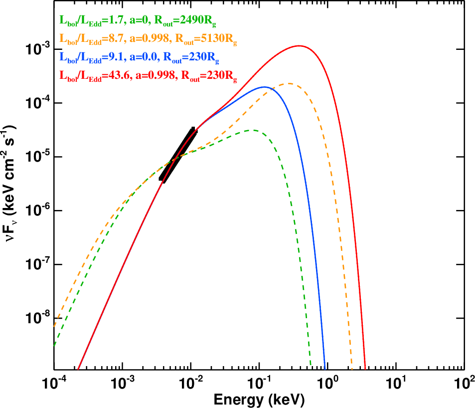
(A colour version of this figure is available in the online journal.)
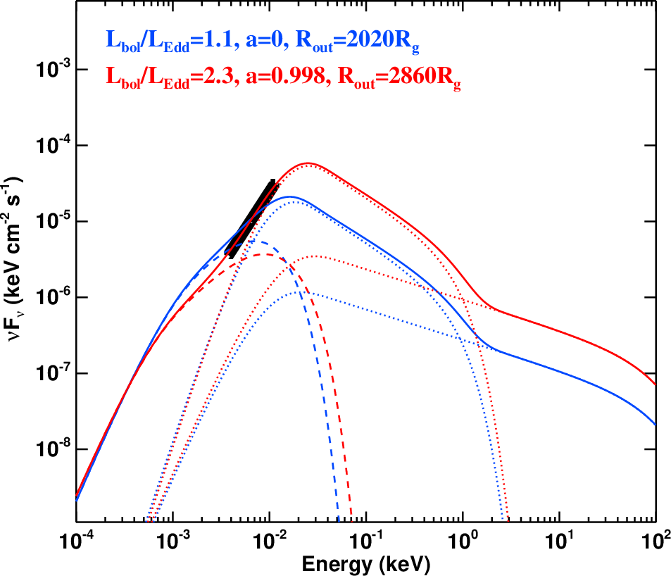
(A colour version of this figure is available in the online journal.)
| Model | |||||
|---|---|---|---|---|---|
| () | () | ||||
| SED-1 | 1.7 | 0f | – | 2490s | 319.0/19 |
| SED-2 | 8.7 | 0.998f | – | 5130s | 297.4/19 |
| SED-3 | 9.1 | 0f | – | 228 | 3.7/18 |
| SED-4 | 43.6 | 0.998f | – | 227 | 3.6/18 |
| SED-5 | 1.1 | 0f | 90.1 | 2020s | 132.5/18 |
| SED-6 | 2.3 | 0.998f | 53.8 | 2860s | 1.5/18 |
4.4 Chemical abundance in BLR
We measure the chemical abundance in the BLR by using the measured emission line flux ratios. The Fe ii/Mg ii ratio indicator is popular for high redshift quasars since Mg ii and Fe ii can be detected in most of their spectra (Sec. 4.4.1). Other metal lines (N v, Si iv+O iv], and He ii) are fainter and sometimes not detected for high-redshift quasars. We can measure those faint lines in our spectrum, and we will utilize their ratios to determine the metallicity (Sec. 4.4.2).
4.4.1 Fe ii/Mg ii
The Fe ii/Mg ii is a simple chemical abundance tracer as described in Sec. 1. The method of fitting the Fe ii template and Mg ii line profile is described in Sec. 3. We integrate the Fe ii template and the double Gaussian function of Mg ii within the rest-frame wavelength range of [2200 – 3090] ÅÅ to calculate the Fe ii flux and Mg ii flux, respectively. The flux error is originated from the uncertainties in the fitting. We show the Fe ii/Mg ii ratios based on two different Mg ii line profile fittings in Table. 4. The comparison between this result and other quasars is discussed in Sec. 5.2.
| Fitted model | Mg ii Flux | Fe ii Flux | Fe ii/Mg ii | |
|---|---|---|---|---|
| (10-16 erg s-1 cm-2) | (10-16 erg s-1 cm-2) | |||
| Mg ii Double Gaussian | ||||
| Mg ii Single Gaussian |
4.4.2 Metallicity
Nagao, Marconi, & Maiolino 2006 (hereafter 51) investigated the relations between metallicity () and several line ratios in the BLR of quasars. Due to the exceptional blue continuum slope in PSO J006+39, we reproduce 51’s work with optimization for this quasar. We adopt the locally optimally emitting cloud (LOC) model (Baldwin et al. 1995) and apply the latest photoionization code Cloudy version 17.01 (Ferland et al. 2013), which is newer than Cloudy version 94.00 used by 51. We note that the latest Cloudy version 17.01 adopts a newer solar elemental abundance table (Grevesse & Sauval 1998) than the older version 94.00. We follow 51’s method to run Cloudy calculations by varying gas densities (), ionizing photon fluxes (), and in the same ranges. The metallicities used in the calculations are 0.2, 0.5, 1.0, 2.0, 5.0, and 10.0 . The stopping conditions and the scaling of metal abundances (the secondary Nitrogen abundances) in the calculations are the same as those in 51. 51 assumed two SEDs for AGNs, the typical SED and the typical SED plus a large UV bump, in their Cloudy calculations. We adopt their SED with the large UV bump, but alter the slope to the same blueness as seen in PSO J006+39 between the lowest rest-frame energy in the observed NIR spectrum and the turning point at 1 Rydberg (Ry) in their SED. Fig. 7 shows the difference between the SED with large UV bump in 51 and the bluer SED we created. We integrate the line intensity using equation (2) in 51; i.e.,
| (3) |
where and are the cloud distribution functions for radius () and . Baldwin et al. 1995 assumed and . We follow 51 by adopting and in the integration of Eq. 3 . Fig. 8 shows the line ratios as a function of metallicities from our Cloudy calculations. We find that the results are different between the same SED but different Cloudy versions. Our results from latest Cloudy version show that N v/C iv and N v/He ii line ratios are positively correlated with the metallicity, while He ii/C iv line ratio is negatively correlated with the metallicity. Besides, (Si iv+O iv])/C iv, (O i+Si ii)/C iv and C iii]/C iv line ratios show only weak correlation with metallicity. By adopting the calculations between observed line ratios and predicted ratios from different metallicities, our result show with the smallest for . The interpretation of these results is described in Sec. 5.2.

(A colour version of this figure is available in the online journal.)

(A colour version of this figure is available in the online journal.)
5 Discussion
5.1 Implication of the blue continuum slope
Fig. 9 shows the continuum slope versus bolometric luminosity () estimated from a linear scaling of 3000Å luminosity following Shen et al. 2008 for quasars. There are only a few objects with continuum slopes bluer than (Jiang et al. 2007; De Rosa et al. 2011; De Rosa et al. 2014). This is typical of lower redshift quasars also (Xie et al. 2016). Davis, Woo, & Blaes 2007 show that there are very few quasars around which have spectra equivalently as blue as a disc (). Much of this discrepancy can be due to dust in the host galaxy causing reddening of the quasar (Richards et al. 2003; Davis, Woo, & Blaes 2007, e.g.). It may be that dust on large scales in the host galaxy has yet to form at the extremely high redshifts probed here, although it is clear that the central regions have metallicity close to or beyond solar (Sec. 4.4.2; see also Sec. 5.2).
Nonetheless, none of the quasars in the SDSS sample of Davis, Woo, & Blaes 2007 have spectra as blue as PSO J006+39 (equivalent to ). We speculated in Sec. 4.3 that this may be produced if the accretion flow is highly super-Eddington, resulting in the inner accretion flow puffing up into a funnel. The apparently small outer radius seen in our spectral fits is then set by the outer edge of the funnel rather than by the outer disc itself, and emission from inside the funnel is geometrically beamed by the opening angle of the funnel (King et al. 2001). We note that Wang et al. 2014 calculated spectral models of a super-Eddington disc, but ignore the effect of reflection from the funnel, so their models remain rather red.
The uniquely blue spectral index of PSO J006+39 comes then from a combination of factors, firstly the flow has to be highly super-Eddington in order to puff up into a funnel, and secondly our line of sight has to intersect this smaller solid angle. The flow is super-Eddington even at low spin (). However, local, lower mass AGNs which appear similarly super-Eddington do not show such blue spectra (Jin et al. 2017b, e.g. RXJ0439 with has ,). Note that in their work is equivalent to in this work. This could support an argument for high black hole spin in PSO J006+39 as then the same outer disc mass accretion rate (which is constrained by the data) leads to a larger bolometric flux so it is more super-Eddington (e.g. with maximal spin we have ). This is more extreme than any local AGN, so would give a more extreme accretion geometry.
The very blue slope also has implications for the ionising flux from AGN in the early Universe. Simulations predict that the dominant population at are from low mass black holes accreting at high Eddington fractions (Fanidakis 2011, e.g.). This makes them similar to the local Narrow Line Seyfert 1 (NLS1) class of AGN, and potentially similar to PSO J006+39 but at lower mass. The NLS1 in the local Universe have spectra which are much more EUV bright than the standard AGN template spectra such as that shown as the black line in Fig. 7 (Casebeer, Leighly, & Baron 2006, see e.g. Fig. 6 in). Thus their contribution to reionisation of hydrogen/helium in the early universe is severely underestimated by the standard template AGN spectral energy distribution (Haardt & Madau 2012, e.g.). However, if the disc puffs up then the escape fraction from the AGN is low, so that their contribution is suppressed. More physical models of the AGN spectra and geometry are required in order to properly calculate their contribution to reionisation at high redshift.
Black hole spin plays a large role in the formation and evolution of SMBHs. Many models assume that the growth rate of the black hole is limited to , which is lower for higher black hole spin due to the increased efficiency, . is the speed of light. With this condition it is hard to form massive quasars at from accretion onto low mass black hole seeds in the early Universe. However, the observation that flows in the local universe can be super-Eddington shows that it is likely that black holes can grow at super-Eddington rates with sufficient gas supply (Jin, Done, & Ward 2016; Jin et al. 2017b).
Recently there have been multiple efforts to understand how black hole mass accretion rate and spin evolve as the SMBH and their host galaxy grow from the early Universe to the present day (Volonteri et al. 2005; Sijacki, Springel, & Haehnelt 2009; Fanidakis et al. 2011; Griffin et al. 2018, e.g.). Gas accretion in a fixed plane spins up the black hole, leading to maximal spin when the black hole mass doubles, but separate small accretion episodes with random angular momentum can lead to random walk spin-up/spin down, resulting in low black hole spin. The supply of gas is linked to the host galaxy and its evolution, with major mergers leading to widespread star formation, triggering gas flows into the nucleus to power the accretion fed growth of the black hole. These also eventually lead to black hole-black hole mergers, which also affect the spin distribution. Such models predict a link between black hole spin and host galaxy morphology, though they are dependent on multiple assumptions (Sesana et al. 2014; Griffin et al. 2018, e.g.).
If the black hole is indeed high spin then we might expect that it can power a strong jet. The Blandford-Znajek (BZ) mechanism (Blandford & Znajek 1977) claims that high black hole spin and the strong magnetic field are two critical physical properties to produce a powerful jet in an AGN. Given the high Eddington ratio that we obtain from the SED fitting in Sec. 4.3, PSO J006+39 may fit in the scenario of super-Eddington ratio with slim accretion disk that can produce jet (Tchekhovskoy 2015) if the magnetic field is strong. Currently, we only know a few quasars that may have jets in the high-redshift universe. In Bañados et al. 2015 they reported only nine radio-loud quasars found at , corresponding to among total high redshift quasars. It is still unclear that whether PSO J006+39 is radio loud or quiet. There is no signal from PSO J006+39 in the TIFR GMRT Sky Survey (Intema et al. 2017, TGSS;) carried out at the Giant Metrewave Radio Telescope (Swarup et al. 1991, GMRT;) at 150 MHz. The detection limit of TGSS is 5 mJy beam-1. With an extrapolation of the slope in the NIR spectrum to 4400Å, the radio loudness is below for PSO J006+39. Therefore, whether it is a radio-loud quasar still awaits future observations to confirm.

(A colour version of this figure is available in the online journal.)
5.2 BLR’s chemical abundance in PSO J006+39

(A colour version of this figure is available in the online journal.)

(A colour version of this figure is available in the online journal.)
We first examine the chemical abundance of PSO J006+39. The photoionization calculations show that the actual metallicity is likely , while the smallest among all metallicities is found at (Sec. 4.4.2). In Fig. 8, most of the observed line ratios fall in this metallicity range except for He ii/C iv and (O i+Si ii)/C iv line ratios. These discrepancies between the line ratios are probably due to the simple assumption of indices ( and ) in the line integration (see 51 for more discussions). Although there is ambiguity in the metallicity value, PSO J006+39 is very likely to have a super solar metallicity in the BLR. This is consistent with the result from Jiang et al. 2007 that quasars typically have super solar () metallicities.
We now compare PSO J006+39 with other quasars to find out whether it has lower chemical abundance. Given that there is no strong evidence so far for high redshift quasars showing lower chemical abundance than low redshift quasars (Sec. 1), finding a low metallicity quasar at high redshift may reveal the reason behind this discrepancy between theoretical prediction and observational evidence. We show the Fe ii/Mg ii line ratio comparison between PSO J006+39 and quasars at with available Fe ii/Mg ii line ratio in Fig. 10. We find that PSO J006+39 has relatively low Fe ii/Mg ii line ratio comparing to quasars at if we adopt the result from the double Gaussian fitting for Mg ii. We caution that this result could be strongly affected by different assumptions in the fittings. For example, 49 assumed 10% of normalization factor for Balmer pseudo-continuum while both De Rosa et al. 2011 and De Rosa et al. 2014 assumed 30%. We adopt a double Gaussian function for Mg ii line fitting while 49 adopted a single Gaussian function. Jiang et al. 2007 stated that they applied Gaussian convolution on the Fe ii template without showing specific value while De Rosa et al. 2011 specifically mentioned that they applied FWHM=15Å. The small uncertainty in our result may be due to the better SNR in our data comparing to the data used by 49, but this does not include all these systematic errors.
We also directly compare individual line ratios between quasars studied so far and PSO J006+39. This may be useful because 51 found that different line ratios have different relations with metallicities. We show the line ratio as a function of redshift in Fig. 11 and as a function of in Fig. 12. The selected quasar samples include nearby AGNs (Shin et al. 2013), nitrogen-loud SDSS quasars (Batra & Baldwin 2014), SDSS quasars with NIR spectra (Juarez et al. 2009), and quasars (Jiang et al. 2007; De Rosa et al. 2014). In addition, the SDSS low redshift () quasar sample is classified into different luminosity groups according to 51. In Fig. 11, we find that both N v/C iv and He ii/C iv line ratios of PSO J006+39 show lower values while other line ratios of this quasar show similar values comparing to quasars from 51 and Batra & Baldwin 2014. Other quasar samples are roughly consistent with PSO J006+39. We also find that the quasars with the UV continuum slopes bluer than the 59 model do not show significantly different line ratios comparing to redder quasars in Fig. 11. This is consistent with the results shown in Fig. 8. From the comparison in Fig. 11, we find different interpretations for the metallicity of PSO J006+39 using different line ratio indicators. With the lower value in N v/C iv ratio, our Cloudy calculation (Fig. 8) suggests that PSO J006+39 indicates lower metallicity comparing to most quasars. However, Fig. 8 suggests that the lower value of PSO J006+39 in He ii/C iv ratio also indicates slightly higher metallicity comparing to most quasars while the similar value in N v/He ii has similar metallicity. It is possible that metal abundance pattern in the BLR of quasars is different from the solar metal abundance pattern.
We address potential issues in measuring metallicity by using the metal line flux ratios. First, since luminosity (51) and (Matsuoka et al. 2011, see also Fig. 12) both have relations with the metallicities in the BLR of quasars, we should select quasars with similar luminosity and group for fair metallicity comparison. However, after extrapolating the power-law continuum of this quasar to optical blue absolute magnitude (), we find that the of PSO J006+39 is fainter () than any luminosity group presented by 51 . In addition, due to the large uncertainties in the measurements, grouping of quasars in terms of similar is difficult. Second, it is doubtful to use the nitrogen lines in metallicity determination for nitrogen-loud quasars (Hamann et al. 2002; Jiang, Fan, & Vestergaard 2008, e.g.). It is possible that strong nitrogen lines are due to the nitrogen overabundance than expected from ordinary scaling relation between N/O and O/H, instead of the overall high metallicity. Since PSO J006+39 is not a nitrogen-loud quasar (no detection of N iv] and N iii] and no prominent broad emission line of N v), the lower N v/C iv ratio of this quasar comparing to the nitrogen-loud quasars from Batra & Baldwin 2014 may be caused by their unusual nitrogen abundances. In this sense, PSO J006+39 can be compared to stacked quasar spectra in 51 in which the contribution from nitrogen-loud quasars are likely small, because nitrogen-loud quasars comprise only 1% of SDSS quasars even though EW of nitrogen emission line in nitrogen-loud quasars are one order of magnitude higher than nitrogen quiet (Jiang, Fan, & Vestergaard 2008). In comparison with 51, N v/C iv in Fig. 11 indicates that the metallicity of PSO J006+39 is lower than that of quasars in 51 in contrast to relatively higher metallicity in He ii/C iv, when we use the newest version of the cloudy. These trends are similar to that we found in comparison with nitrogen-loud quasars. This suggests that the potential issue behind the comparison in Fig. 11 might include not only the unusual nitrogen abundance but also the difficulty of accurate modelling of emission lines of BRLs. Actually we found that He ii/C iv-metallicity relation dramatically changed from the correlation to anti-correlation depending on the different versions of cloudy as shown in the top-middle panel in Fig. 8.

(A colour version of this figure is available in the online journal.)
6 Conclusions
We found that PSO J006+39 has a relatively less massive () and an exceptionally blue power-law continuum slope () compared to other quasars at . We performed SED model fitting and find that this blue continuum slope can be explained by the accretion disc model proposed by Done et al. 2012 with a very small disc (). This is perhaps due to the flow puffing up into a funnel which is most easily explained if the black hole has high spin and the flow is highly super-Eddington () according to King et al. 2001. This indicates the high spin at such high redshift for the first time, and appears consistent with the models of black hole spin evolution proposed by Sesana et al. 2014. Our analysis showed that this quasar exhibits super solar metallicity based on our photoionization calculations, but the measured Fe ii/Mg ii line ratio is relatively low compared to known quasars. However, other different line ratios indicate different metallicities. Therefore, we could not confirm whether this quasar has lower metallicity compared to other quasars.
Acknowledgements
We thank the Gemini staffs in preparing and carrying out the observations. We thank the anonymous referees for many insightful comments. We acknowledge K. Matsuoka, Y. Matsuoka, T. Nagao, M. Nakamura, A. Schulze, X. B. Wu, R. Momose for useful discussions. TG acknowledges the support by the Ministry of Science and Technology of Taiwan (MoST) through grant 105-2112-M-007-003-MY3, and YO acknowledges the support by the MoST of Taiwan through grant 106-2112-M-001-008- and 107-2119-M-001-026-. CJ is supported by the Hundred Talents Program of the Chinese Academy of Sciences. CJ acknowledges the National Natural Science Foundation of China through grant 11873054. CD acknowledges the Science and Technology Facilities Council (STFC) through grant ST/P000541/1 for support. EKE acknowledges a post-doctoral fellowship from TUBITAK-BIDEB through 2218 program.
References
- Baldwin et al. (1995) Baldwin J., Ferland G., Korista K., Verner D., 1995, ApJ, 455, L119
- Bañados et al. (2015) Bañados E., et al., 2015, ApJ, 804, 118
- Bañados et al. (2016) Bañados E., et al., 2016, ApJS, 227, 11
- Bañados et al. (2018) Bañados E., et al., 2018, Natur, 553, 473
- Barth et al. (2003) Barth A. J., Martini P., Nelson C. H., Ho L. C., 2003, ApJ, 594, L95
- Batra & Baldwin (2014) Batra N. D., Baldwin J. A., 2014, MNRAS, 439, 771
- Bentz et al. (2013) Bentz M. C., et al., 2013, ApJ, 767, 149
- Blandford & Znajek (1977) Blandford R. D., Znajek R. L., 1977, MNRAS, 179, 433
- Campitiello et al. (2018) Campitiello S., Ghisellini G., Sbarrato T., Calderone G., 2018, A&A, 612, A59
- Casebeer, Leighly, & Baron (2006) Casebeer D. A., Leighly K. M., Baron E., 2006, ApJ, 637, 157
- Collin & Kawaguchi (2004) Collin S., Kawaguchi T., 2004, A&A, 426, 797
- Collinson et al. (2017) Collinson J. S., Ward M. J., Landt H., Done C., Elvis M., McDowell J. C., 2017, MNRAS, 465, 358
- Davis, Woo, & Blaes (2007) Davis S. W., Woo J.-H., Blaes O. M., 2007, ApJ, 668, 682
- Davis & Laor (2011) Davis S. W., Laor A., 2011, ApJ, 728, 98
- De Rosa et al. (2011) De Rosa G., Decarli R., Walter F., Fan X., Jiang L., Kurk J., Pasquali A., Rix H. W., 2011, ApJ, 739, 56
- De Rosa et al. (2014) De Rosa G., et al., 2014, ApJ, 790, 145
- Diamond-Stanic et al. (2009) Diamond-Stanic A. M., et al., 2009, ApJ, 699, 782
- Dietrich et al. (2003) Dietrich M., Hamann F., Appenzeller I., Vestergaard M., 2003, ApJ, 596, 817
- Done et al. (2012) Done C., Davis S. W., Jin C., Blaes O., Ward M., 2012, MNRAS, 420, 1848
- Gallerani et al. (2010) Gallerani S., et al., 2010, A&A, 523, A85
- Grandi (1982) Grandi S. A., 1982, ApJ, 255, 25
- Grevesse & Sauval (1998) Grevesse N., Sauval A. J., 1998, SSRv, 85, 161
- Griffin et al. (2018) Griffin A. J., Lacey C. G., Gonzalez-Perez V., Lagos C. d. P., Baugh C. M., Fanidakis N., 2018, arXiv, arXiv:1806.08370
- Fanidakis (2011) Fanidakis N., 2011, PhDT,
- Fanidakis et al. (2011) Fanidakis N., Baugh C. M., Benson A. J., Bower R. G., Cole S., Done C., Frenk C. S., 2011, MNRAS, 410, 53
- Ferland et al. (2013) Ferland G. J., et al., 2013, RMxAA, 49, 137
- Freudling, Corbin, & Korista (2003) Freudling W., Corbin M. R., Korista K. T., 2003, ApJ, 587, L67
- Haardt & Madau (2012) Haardt F., Madau P., 2012, ApJ, 746, 125
- Hagino et al. (2017) Hagino K., Done C., Odaka H., Watanabe S., Takahashi T., 2017, MNRAS, 468, 1442
- Hamann et al. (2002) Hamann F., Korista K. T., Ferland G. J., Warner C., Baldwin J., 2002, ApJ, 564, 592
- Hao et al. (2010) Hao H., et al., 2010, ApJ, 724, L59
- Leighly (2004) Leighly K. M., 2004, ApJ, 611, 125
- Intema et al. (2017) Intema H. T., Jagannathan P., Mooley K. P., Frail D. A., 2017, A&A, 598, A78
- Iwamuro et al. (2002) Iwamuro F., Motohara K., Maihara T., Kimura M., Yoshii Y., Doi M., 2002, ApJ, 565, 63
- Iwamuro et al. (2004) Iwamuro F., Kimura M., Eto S., Maihara T., Motohara K., Yoshii Y., Doi M., 2004, ApJ, 614, 69
- Jiang et al. (2007) Jiang L., Fan X., Vestergaard M., Kurk J. D., Walter F., Kelly B. C., Strauss M. A., 2007, AJ, 134, 1150
- Jiang, Fan, & Vestergaard (2008) Jiang L., Fan X., Vestergaard M., 2008, ApJ, 679, 962
- Jin, Done, & Ward (2016) Jin C., Done C., Ward M., 2016, MNRAS, 455, 691
- Jin, Done, & Ward (2017a) Jin C., Done C., Ward M., 2017a, MNRAS, 468, 3663
- Jin et al. (2017b) Jin C., Done C., Ward M., Gardner E., 2017b, MNRAS, 471, 706
- Juarez et al. (2009) Juarez Y., Maiolino R., Mujica R., Pedani M., Marinoni S., Nagao T., Marconi A., Oliva E., 2009, A&A, 494, L25
- Kaiser et al. (2002) Kaiser N., et al., 2002, SPIE, 4836, 154
- Kaiser et al. (2010) Kaiser N., et al., 2010, SPIE, 7733, 77330E
- King et al. (2001) King A. R., Davies M. B., Ward M. J., Fabbiano G., Elvis M., 2001, ApJ, 552, L109
- Kubota & Done (2018) Kubota A., Done C., 2018, MNRAS, 480, 1247
- Maiolino et al. (2003) Maiolino R., Juarez Y., Mujica R., Nagar N. M., Oliva E., 2003, ApJ, 596, L155
- Matsuoka et al. (2011) Matsuoka K., Nagao T., Marconi A., Maiolino R., Taniguchi Y., 2011, A&A, 527, A100
- Matteucci & Greggio (1986) Matteucci F., Greggio L., 1986, A&A, 154, 279
- Mazzucchelli et al. (2017) Mazzucchelli C., et al., 2017, ApJ, 849, 91
- McWilliam (1997) McWilliam A., 1997, ARA&A, 35, 503
- Nagao, Marconi, & Maiolino (2006) Nagao T., Marconi A., Maiolino R., 2006, A&A, 447, 157
- Petrucci et al. (2018) Petrucci P.-O., Ursini F., De Rosa A., Bianchi S., Cappi M., Matt G., Dadina M., Malzac J., 2018, A&A, 611, A59
- Richards et al. (2003) Richards G. T., et al., 2003, AJ, 126, 1131
- Richards et al. (2011) Richards G. T., et al., 2011, AJ, 141, 167
- Selsing et al. (2016) Selsing J., Fynbo J. P. U., Christensen L., Krogager J.-K., 2016, A&A, 585, A87
- Sesana et al. (2014) Sesana A., Barausse E., Dotti M., Rossi E. M., 2014, ApJ, 794, 104
- Sijacki, Springel, & Haehnelt (2009) Sijacki D., Springel V., Haehnelt M. G., 2009, MNRAS, 400, 100
- Shankar et al. (2016) Shankar F., et al., 2016, ApJ, 818, L1
- Shakura & Sunyaev (1973) Shakura N. I., Sunyaev R. A., 1973, A&A, 24, 337
- Shen et al. (2008) Shen Y., Greene J. E., Strauss M. A., Richards G. T., Schneider D. P., 2008, ApJ, 680, 169-190
- Shin et al. (2013) Shin J., Woo J.-H., Nagao T., Kim S. C., 2013, ApJ, 763, 58
- Swarup et al. (1991) Swarup G., Ananthakrishnan S., Kapahi V. K., Rao A. P., Subrahmanya C. R., Kulkarni V. K., 1991, CuSc, 60, 95
- Tang et al. (2017) Tang J.-J., et al., 2017, MNRAS, 466, 4568
- Tchekhovskoy (2015) Tchekhovskoy A., 2015, ASSL, 414, 45
- Vanden Berk et al. (2001) Vanden Berk D. E., et al., 2001, AJ, 122, 549
- Venemans et al. (2016) Venemans B. P., Walter F., Zschaechner L., Decarli R., De Rosa G., Findlay J. R., McMahon R. G., Sutherland W. J., 2016, ApJ, 816, 37
- Vestergaard & Wilkes (2001) Vestergaard M., Wilkes B. J., 2001, ApJS, 134, 1
- Vestergaard & Osmer (2009) Vestergaard M., Osmer P. S., 2009, ApJ, 699, 800
- Volonteri et al. (2005) Volonteri M., Madau P., Quataert E., Rees M. J., 2005, ApJ, 620, 69
- Wang et al. (2014) Wang J.-M., Qiu J., Du P., Ho L. C., 2014, ApJ, 797, 65
- Wu et al. (2015) Wu X.-B., et al., 2015, Natur, 518, 512
- Woo et al. (2018) Woo J.-H., Le H. A. N., Karouzos M., Park D., Park D., Malkan M. A., Treu T., Bennert V. N., 2018, ApJ, 859, 138
- Xie et al. (2016) Xie X., Shao Z., Shen S., Liu H., Li L., 2016, ApJ, 824, 38
- Xu et al. (2018) Xu F., Bian F., Shen Y., Zuo W., Fan X., Zhu Z., 2018, MNRAS, 480, 345