跳到论文正文
W Papers独立论文阅读器 arXiv:1901.02581 论文正文 计算阅读时间 · 0%
引用这篇论文根据当前论文元数据生成,正式投稿前建议核对。


License: arXiv.org perpetual non-exclusive license
arXiv:1901.02581v2 [math.DS] 02 Aug 2019

Ultradiscrete two-variable Oregonator

Yuhei KASHIWATATE
Abstract

Ultradiscretization is a limiting procedure transforming a given differential/difference equation into a ultradiscrete equation. Ultradiscrete equations are expressed by addition, subtraction and/or max. The procedure is expected to preserve the essential properties of the original equations. As a method of ultradiscretization, there is “tropical discretization” proposed by M. Murata. In this paper, we shall modify it, and derive a ultradiscrete equation from the continuous model of the BZ reaction. The derived equation generates a cellular automaton by restricting the values of the parameters, which is equivalent to one of those introduced by D. Takahashi, A. Shida, and M. Usami. By setting appropriate initial values, we can obtain the typical patterns of the BZ reaction. Furthermore, we consider the equation without diffusion effect and derive the explicit solutions. As a result, the solutions corresponding to the limit cycle (oscillation) appearing in the continuous model will be found.
MSC: 39A12; 39A14, 35K57.
Key words: discretization, ultradiscrete equation, BZ reaction, cellular automaton.

Graduate School of Science and Engineering, Yamagata University, Kojirakawa-machi 1-4-12, Yamagata 990-8560, Japan

E-mail: s181104m@st.yamagata-u.ac.jp

1 Introduction

Ultradiscretization is a limiting procedure transforming a given differential/diffe- rence equation into a ultradiscrete equation. Ultradiscrete equations are based on the max-plus algebra, which defines the summation by max and the product by +, and often expressed in simple forms. It is expected that this procedure preserves the essential properties of the original equations. In the reaction-diffusion system, both continuous models using partial differential equations and mathematical models using cellular automatons have been studied. However, the direct correspondence between them is not clear. Indeed, it was difficult to obtain max-plus equations expressing the BZ reaction directly from the system of partial differential equations. For example, in their paper [3], D. Takahashi, A. Shida, and M. Usami created max-plus equations for the BZ reaction simply by comparing its typical nature.

As a method of ultradiscretization, there is “tropical discretization” proposed by M. Murata [1, 2]. In this paper, we shall modify it, and derive a ultradiscrete equation from the continuous model of the BZ reaction. Ultradiscretization of two-dimensional space diffusion terms will be the mean of values of neighbouring four points and center. In Murata’s method, the value of center is not used. Another difference is which terms are shifted in time. The derived equation generates a cellular automaton by restricting the values of the parameters, which is equivalent to one of those introduced in the paper [3]. By setting appropriate initial values, we obtain the typical patterns of the BZ reaction, ring, target and spiral, which are mentioned in the book [4].

Furthermore, we consider the equation without diffusion effect and derive the explicit solutions. As a result, the solutions corresponding to the limit cycle (oscillation) appearing in the continuous model will be found.

2 The two-variable Oregonator

The two-variable Oregonator in two-dimensional space is given by

{∂u∂t=Du​(∂2u∂x2+∂2u∂y2)+a⁡{u⁡(1−u)−f​v​(u−q)u+q},∂v∂t=Dv​(∂2v∂x2+∂2v∂y2)+u−v,\left\{\begin{aligned} \frac{\partial u}{\partial t}&=D_{u}\left(\frac{\partial^{2}u}{\partial x^{2}}+\frac{\partial^{2}u}{\partial y^{2}}\right)+a\left\{u(1-u)-\frac{fv(u-q)}{u+q}\right\},\\ \frac{\partial v}{\partial t}&=D_{v}\left(\frac{\partial^{2}v}{\partial x^{2}}+\frac{\partial^{2}v}{\partial y^{2}}\right)+u-v,\end{aligned}\right. (2.1)

where u=u⁡(t,x,y)u=u(t,x,y) is the activity factor and v=v⁡(t,x,y)v=v(t,x,y) is the inhibitory factor. The constants DuD_{u} and DvD_{v} are the diffusion coefficients of uu and vv, respectively. We consider (x,y)∈ℝ2,t≥0(x,y)\in\mathbb{R}^{2},\>t\geq 0 and the constants a,f,qa,f,q satisfy a∼0.25×10², 1<f<2,q∼8×10⁻⁴a\sim 0.25\times 10^{2},\>1<f<2,\>q\sim 8\times 10^{-4}. This system is known as a model to explain the pattern dynamics of the BZ reaction. The solutions of this system represent spatial patterns. Changing initial values and the values of paremeters, we can observe various patterns.

2.1 Discretization

In this section, we discretize the eq.(2.1) by a method similar to Murata’s [1]. First we consider a discretization of the following system of partial differential equations:

{∂u∂t=Du​(∂2u∂x2+∂2u∂y2)(Du>0),∂v∂t=Dv​(∂2v∂x2+∂2v∂y2)(Dv>0).\begin{cases}{\displaystyle{\displaystyle\frac{\partial u}{\partial t}}=D_{u}\left({\displaystyle\frac{\partial^{2}u}{\partial x^{2}}+\frac{\partial^{2}u}{\partial y^{2}}}\right)}&(D_{u}>0),\\ {\displaystyle{\displaystyle\frac{\partial v}{\partial t}}=D_{v}\left({\displaystyle\frac{\partial^{2}v}{\partial x^{2}}+\frac{\partial^{2}v}{\partial y^{2}}}\right)}&(D_{v}>0).\end{cases} (2.2)

The following system of difference equations is that.

{un+1j,k=15​(unj,k+unj−α,k+unj+α,k+unj,k−α+unj,k+α)=mα​(unj,k),vn+1j,k=15​(vnj,k+vnj−β,k+vnj+β,k+vnj,k−β+vnj,k+β)=mβ​(vnj,k).\left\{\begin{aligned} u_{n+1}^{j,k}&=\frac{1}{5}(u_{n}^{j,k}+u_{n}^{j-\alpha,k}+u_{n}^{j+\alpha,k}+u_{n}^{j,k-\alpha}+u_{n}^{j,k+\alpha})=m_{\alpha}(u_{n}^{j,k}),\\ v_{n+1}^{j,k}&=\frac{1}{5}(v_{n}^{j,k}+v_{n}^{j-\beta,k}+v_{n}^{j+\beta,k}+v_{n}^{j,k-\beta}+v_{n}^{j,k+\beta})=m_{\beta}(v_{n}^{j,k}).\end{aligned}\right. (2.3)

Indeed, if we put unj,k=u⁡(t,x,y)u_{n}^{j,k}=u(t,x,y) with t=n​Δ​t,x=j​Δ​x,y=k​Δ​y​(Δ​x=Δ​y)t=n\Delta t,\>x=j\Delta x,\>y=k\Delta y\>(\Delta x=\Delta y), we find

un+1j,k\displaystyle u_{n+1}^{j,k} =u⁡(t+Δ​t,x,y),\displaystyle=u(t+\Delta t,x,y),
unj±α,k\displaystyle u_{n}^{j\pm\alpha,k} =u⁡(t,x±α​Δ​x,y),\displaystyle=u(t,x\pm\alpha\Delta x,y),
unj,k±α\displaystyle u_{n}^{j,k\pm\alpha} =u⁡(t,x,y±α​Δ​y).\displaystyle=u(t,x,y\pm\alpha\Delta y).

By the taylor expansions at (t,x,y)(t,x,y), we get

u⁡(t,x,y)\displaystyle u(t,x,y) =u,\displaystyle=u,
u⁡(t+Δ​t,x,y)\displaystyle u(t+\Delta t,x,y) =u+ut​Δ​t+12​ut​t​Δ​t2+⋯,\displaystyle=u+u_{t}\Delta t+\frac{1}{2}u_{tt}\Delta t^{2}+\cdots,
u⁡(t,x±α​Δ​x,y)\displaystyle u(t,x\pm\alpha\Delta x,y) =u±ux​α​Δ​x+12​ux​x​α2​Δ​x2±⋯,\displaystyle=u\pm u_{x}\alpha\Delta x+\frac{1}{2}u_{xx}\alpha^{2}\Delta x^{2}\pm\cdots,
u⁡(t,x,y±α​Δ​y)\displaystyle u(t,x,y\pm\alpha\Delta y) =u±uy​α​Δ​y+12​uy​y​α2​Δ​y2±⋯.\displaystyle=u\pm u_{y}\alpha\Delta y+\frac{1}{2}u_{yy}\alpha^{2}\Delta y^{2}\pm\cdots.

Substituting them into the eq.(2.3), we get

u+ut​Δ​t+12​ut​t​Δ​t2+⋯=15\displaystyle u+u_{t}\Delta t+\frac{1}{2}u_{tt}\Delta t^{2}+\cdots=\frac{1}{5} {u+(u+uxαΔx+12ux​xα2Δx2+⋯)\displaystyle\left\{u+\left(u+u_{x}\alpha\Delta x+\frac{1}{2}u_{xx}\alpha^{2}\Delta x^{2}+\cdots\right)\right.
+(u−ux​α​Δ​x+12​ux​x​α2​Δ​x2−⋯)\displaystyle\left.+\left(u-u_{x}\alpha\Delta x+\frac{1}{2}u_{xx}\alpha^{2}\Delta x^{2}-\cdots\right)\right.
+(u+uy​α​Δ​y+12​uy​y​α2​Δ​y2+⋯)\displaystyle\left.+\left(u+u_{y}\alpha\Delta y+\frac{1}{2}u_{yy}\alpha^{2}\Delta y^{2}+\cdots\right)\right.
+(u−uyαΔy+12uy​yα2Δy2−⋯)},\displaystyle\left.+\left(u-u_{y}\alpha\Delta y+\frac{1}{2}u_{yy}\alpha^{2}\Delta y^{2}-\cdots\right)\right\},

and thus

ut​Δ​t+⋯=\displaystyle u_{t}\Delta t+\cdots= 15​ux​x​α2​Δ​x2+15​uy​y​α2​Δ​y2+⋯,\displaystyle\frac{1}{5}u_{xx}\alpha^{2}\Delta x^{2}+\frac{1}{5}u_{yy}\alpha^{2}\Delta y^{2}+\cdots,
ut+⋯=\displaystyle u_{t}+\cdots= α2​Δ​x25​Δ​t​ux​x+α2​Δ​y25​Δ​t​uy​y+⋯,\displaystyle\frac{\alpha^{2}\Delta x^{2}}{5\Delta t}u_{xx}+\frac{\alpha^{2}\Delta y^{2}}{5\Delta t}u_{yy}+\cdots, (2.4)

where D=α2​Δ​x2/5​Δ​t=α2​Δ​y2/5​Δ​tD=\alpha^{2}\Delta x^{2}/5\Delta t=\alpha^{2}\Delta y^{2}/5\Delta t. Taking the limit Δ​t,Δ​x,Δ​y→+0\Delta t,\Delta x,\Delta y\rightarrow+0 without change of DD, we obtain the first equation of the system eq.(2.2). Thus, the eq.(2.3) can be regarded as a discretization of the eq.(2.2).

Furthermore, we consider a discretization of the following syestem of ordinary differential equations:

{d​ud​t=a​{u⁡(1−u)−f​v​(u−q)u+q},d​vd​t=u−v.\left\{\begin{aligned} \frac{du}{dt}&=a\left\{u(1-u)-\frac{fv(u-q)}{u+q}\right\},\\ \frac{dv}{dt}&=u-v.\end{aligned}\right. (2.5)

We shall show that the following syestem of difference equations is the required

{un+1=ε−1​un+a​un+a​f​q​vnun+qε−1+a​un+a​f​vnun+q,vn+1=ε−1​vn+unε−1+1,\left\{\begin{aligned} u_{n+1}&=\frac{\varepsilon^{-1}u_{n}+au_{n}+{\displaystyle\frac{afqv_{n}}{u_{n}+q}}}{\varepsilon^{-1}+au_{n}+{\displaystyle\frac{afv_{n}}{u_{n}+q}}},\\ v_{n+1}&=\frac{\varepsilon^{-1}v_{n}+u_{n}}{\varepsilon^{-1}+1},\end{aligned}\right. (2.6)

where n∈ℤ≥0,ε>0n\in\mathbb{Z}_{\geq 0},\>\varepsilon>0. The method we adopt here is the same as that in the papers [1, 2].

Putting un=u⁡(t),vn=v⁡(t),t=ε​nu_{n}=u(t),\>v_{n}=v(t),\>t=\varepsilon n, we find

{u⁡(t+ε)−u⁡(t)ε=a⁡{u⁡(t)​(1−u⁡(t))−f​v​(t)​(u⁡(t)−q)u⁡(t)+q}+O⁡(ε),v⁡(t+ε)−v⁡(t)ε=u⁡(t)−v⁡(t)+O⁡(ε).\left\{\begin{aligned} \frac{u(t+\varepsilon)-u(t)}{\varepsilon}&=a\left\{u(t)(1-u(t))-\frac{fv(t)(u(t)-q)}{u(t)+q}\right\}+O(\varepsilon),\\ \frac{v(t+\varepsilon)-v(t)}{\varepsilon}&=u(t)-v(t)+O(\varepsilon).\end{aligned}\right. (2.7)

Taking the limit ε→+0\varepsilon\rightarrow+0, we obtain the system of differential equations(2.5). Thus, the eq.(2.6) can be regarded as a discretization of the eq.(2.5). Using the eq.(2.3) and the eq.(2.6), we will find the system of difference equations,

{un+1j,k=ϵ−1​mα​(unj,k)+a​mα​(unj,k)+a​f​q​vnj,kmα​(unj,k)+qϵ−1+a​mα​(unj,k)+a​f​vnj,kmα​(unj,k)+q,vn+1j,k=ϵ−1​mβ​(vnj,k)+mβ​(unj,k)ϵ−1+1.\left\{\begin{aligned} u_{n+1}^{j,k}&=\frac{\epsilon^{-1}m_{\alpha}(u_{n}^{j,k})+am_{\alpha}(u_{n}^{j,k})+{\displaystyle\frac{afqv_{n}^{j,k}}{m_{\alpha}(u_{n}^{j,k})+q}}}{\epsilon^{-1}+am_{\alpha}(u_{n}^{j,k})+{\displaystyle\frac{afv_{n}^{j,k}}{m_{\alpha}(u_{n}^{j,k})+q}}},\\ v_{n+1}^{j,k}&=\frac{\epsilon^{-1}m_{\beta}(v_{n}^{j,k})+m_{\beta}(u_{n}^{j,k})}{\epsilon^{-1}+1}.\end{aligned}\right. (2.8)

This can be rewritten as

{un+1j,k−unj,kε=mα​(unj,k)−unj,kε+a⁡{mα​(unj,k)​(1−unj,k)−f​vnj,k​(unj,k−q)mα​(unj,k)+q}+O⁡(ε),vn+1j,k−vnj,kε=mβ​(vnj,k)−vnj,kε+mβ​(unj,k)−vnj,k+O⁡(ε),\left\{\begin{aligned} \frac{u_{n+1}^{j,k}-u_{n}^{j,k}}{\varepsilon}&=\frac{m_{\alpha}(u_{n}^{j,k})-u_{n}^{j,k}}{\varepsilon}+a\left\{m_{\alpha}(u_{n}^{j,k})(1-u_{n}^{j,k})-\frac{fv_{n}^{j,k}(u_{n}^{j,k}-q)}{m_{\alpha}(u_{n}^{j,k})+q}\right\}+O(\varepsilon),\\ \frac{v_{n+1}^{j,k}-v_{n}^{j,k}}{\varepsilon}&=\frac{m_{\beta}(v_{n}^{j,k})-v_{n}^{j,k}}{\varepsilon}+m_{\beta}(u_{n}^{j,k})-v_{n}^{j,k}+O(\varepsilon),\end{aligned}\right. (2.9)

and thus can be regarded as a discretization of the eq.(2.1).

2.2 Ultradiscretization

In this section, we shall ultradiscretize the eq.(2.8) and investigate the solutions. Let

unj,k=exp⁡(Unj,k/λ),vnj,k=exp⁡(Vnj,k/λ),ϵ=exp⁡(E/λ),a=exp⁡(A/λ),f=exp⁡(F/λ),q=exp⁡(Q/λ),\begin{array}[]{ccc}u_{n}^{j,k}=\exp(U_{n}^{j,k}/\lambda),&v_{n}^{j,k}=\exp(V_{n}^{j,k}/\lambda),&\epsilon=\exp(E/\lambda),\\ a=\exp(A/\lambda),&f=\exp(F/\lambda),&q=\exp(Q/\lambda),\end{array} (2.10)

and take the limit λ→+0\lambda\rightarrow+0. Operations such as

limλ→+0λ​log⁡(eA/λ+eB/λ)\displaystyle\lim_{\lambda\rightarrow+0}\lambda\log\left(e^{A/\lambda}+e^{B/\lambda}\right) =max⁡(A,B),\displaystyle=\max(A,B),
limλ→+0λ​log⁡(eA/λ⋅eB/λ)\displaystyle\lim_{\lambda\rightarrow+0}\lambda\log\left(e^{A/\lambda}\cdotp e^{B/\lambda}\right) =A+B,\displaystyle=A+B,
limλ→+0λ​log⁡(eA/λ​/​eB/λ)\displaystyle\lim_{\lambda\rightarrow+0}\lambda\log\left(e^{A/\lambda}\text{/}e^{B/\lambda}\right) =A−B,\displaystyle=A-B,

perform here. Therefore, the eq.(2.8) is transformed into

{Un+1j,k=max⁡{Mα​(Unj,k)−E,A+Mα​(Unj,k),A+F+Q+Vnj,k−max⁡(Mα​(Unj,k),Q)}−max⁡{−E,A+Mα​(Unj,k),A+F+Vnj,k−max⁡(Mα​(Unj,k),Q)},Vn+1j,k=max⁡{Mβ​(Vnj,k)−E,Mβ​(Unj,k)}−max⁡{−E,0},\left\{\begin{aligned} U_{n+1}^{j,k}=&\max\{M_{\alpha}(U_{n}^{j,k})-E,A+M_{\alpha}(U_{n}^{j,k}),A+F+Q+V_{n}^{j,k}-\max(M_{\alpha}(U_{n}^{j,k}),Q)\}\\ &-\max\{-E,A+M_{\alpha}(U_{n}^{j,k}),A+F+V_{n}^{j,k}-\max(M_{\alpha}(U_{n}^{j,k}),Q)\},\\ V_{n+1}^{j,k}=&\max\{M_{\beta}(V_{n}^{j,k})-E,M_{\beta}(U_{n}^{j,k})\}-\max\{-E,0\},\end{aligned}\right. (2.11)

where

{Mα​(Unj,k)=max⁡(Unj,k,Unj−α,k,Unj+α,k,Unj,k−α,Unj,k+α),Mβ​(Vnj,k)=max⁡(Vnj,k,Vnj−β,k,Vnj+β,k,Vnj,k−β,Vnj,k+β),\left\{\begin{aligned} M_{\alpha}(U_{n}^{j,k})=&\max(U_{n}^{j,k},U_{n}^{j-\alpha,k},U_{n}^{j+\alpha,k},U_{n}^{j,k-\alpha},U_{n}^{j,k+\alpha}),\\ M_{\beta}(V_{n}^{j,k})=&\max(V_{n}^{j,k},V_{n}^{j-\beta,k},V_{n}^{j+\beta,k},V_{n}^{j,k-\beta},V_{n}^{j,k+\beta}),\end{aligned}\right.

which is an ultradiscretization of the eq.(2.3).

Taking the limit E→+∞E\rightarrow+\infty, we get

{Un+1j,k=max⁡{Mα​(Unj,k),F+Q+Vnj,k−max⁡(Mα​(Unj,k),Q)}−max⁡{Mα​(Unj,k),F+Vnj,k−max⁡(Mα​(Unj,k),Q)},Vn+1j,k=Mβ​(Unj,k).\left\{\begin{aligned} U_{n+1}^{j,k}=&\max\{M_{\alpha}(U_{n}^{j,k}),F+Q+V_{n}^{j,k}-\max(M_{\alpha}(U_{n}^{j,k}),Q)\}\\ &-\max\{M_{\alpha}(U_{n}^{j,k}),F+V_{n}^{j,k}-\max(M_{\alpha}(U_{n}^{j,k}),Q)\},\\ V_{n+1}^{j,k}=&M_{\beta}(U_{n}^{j,k}).\end{aligned}\right. (2.12)

and the following single ultradiscrete equation:

Un+1j,k=\displaystyle U_{n+1}^{j,k}= max⁡{Mα​(Unj,k),F+Q+Mβ​(Un−1j,k)−max⁡(Mα​(Unj,k),Q)}\displaystyle\max\{M_{\alpha}(U_{n}^{j,k}),F+Q+M_{\beta}(U_{n-1}^{j,k})-\max(M_{\alpha}(U_{n}^{j,k}),Q)\}
−max⁡{Mα​(Unj,k),F+Mβ​(Un−1j,k)−max⁡(Mα​(Unj,k),Q)}.\displaystyle-\max\{M_{\alpha}(U_{n}^{j,k}),F+M_{\beta}(U_{n-1}^{j,k})-\max(M_{\alpha}(U_{n}^{j,k}),Q)\}. (2.13)

3 Cellular automaton

Considering the values of ff and qq in the eq.(2.1), we suppose Q<0<FQ<0<F in the eq.(2.13). We take Q=−1,F=1Q=-1,\>F=1, and restrict initial values to U0j,k,U1j,k∈{−1,0}U_{0}^{j,k},U_{1}^{j,k}\in\{-1,0\} to generate a cellulor automaton. Under this condition, the values of Unj,kU_{n}^{j,k} are restricted to {−1,0}\{-1,0\}. To shift the values to {0,1}\{0,1\}, Let

Wnj,k=Unj,k−Q,W_{n}^{j,k}=U_{n}^{j,k}-Q, (3.1)

and substitute it into the eq.(2.13). We get

Wn+1j,k=\displaystyle W_{n+1}^{j,k}= max⁡{Mα​(Wnj,k),F+Mβ​(Wn−1j,k)−Mα​(Wnj,k)}\displaystyle\max\{M_{\alpha}(W_{n}^{j,k}),F+M_{\beta}(W_{n-1}^{j,k})-M_{\alpha}(W_{n}^{j,k})\}
−max⁡{Mα​(Wnj,k)+Q,F+Mβ​(Wn−1j,k)−Mα​(Wnj,k)}.\displaystyle-\max\{M_{\alpha}(W_{n}^{j,k})+Q,F+M_{\beta}(W_{n-1}^{j,k})-M_{\alpha}(W_{n}^{j,k})\}. (3.2)

Since we find

Mα​(Wnj,k)\displaystyle M_{\alpha}(W_{n}^{j,k}) ∈{0,1},\displaystyle\in\{0,1\},
F+Mβ​(Wn−1j,k)−Mα​(Wnj,k)\displaystyle F+M_{\beta}(W_{n-1}^{j,k})-M_{\alpha}(W_{n}^{j,k}) ∈{0,1,2},\displaystyle\in\{0,1,2\},
Mα​(Wnj,k)+Q\displaystyle M_{\alpha}(W_{n}^{j,k})+Q ∈{−1,0},\displaystyle\in\{-1,0\},

it follows that

F+Mβ​(Wn−1j,k)−Mα​(Wnj,k)≥Mα​(Wnj,k)+Q.F+M_{\beta}(W_{n-1}^{j,k})-M_{\alpha}(W_{n}^{j,k})\geq M_{\alpha}(W_{n}^{j,k})+Q.

Therefore, we obtain the following simple equation:

Wn+1j,k=max⁡{2​Mα​(Wnj,k)−Mβ​(Wn−1j,k)−F,0}.W_{n+1}^{j,k}=\max\{2M_{\alpha}(W_{n}^{j,k})-M_{\beta}(W_{n-1}^{j,k})-F,0\}. (3.3)

The rule of time evolution is in the Table 3.1:

Mα​(Wnj,k),Mβ​(Wn−1j,k)M_{\alpha}(W_{n}^{j,k}),M_{\beta}(W_{n-1}^{j,k}) 0,00,0 0,10,1 1,01,0 1,11,1
Wn+1j,kW_{n+1}^{j,k} 00 00 11 00
Table 3.1: Wn+1j,kW_{n+1}^{j,k}

We shall compare it with one of Takahashi, Shida and Usami’s max-plus equations [3]:

Yn+1j,k=max⁡(Ynj,k,Ynj−1,k,Ynj+1,k,Ynj,k−1,Ynj,k+1,Yn−1j,k)−Yn−1j,k.Y_{n+1}^{j,k}=\max(Y_{n}^{j,k},Y_{n}^{j-1,k},Y_{n}^{j+1,k},Y_{n}^{j,k-1},Y_{n}^{j,k+1},Y_{n-1}^{j,k})-Y_{n-1}^{j,k}. (3.4)

We recall thet this equation was not associated with the differential equation directly. Using our terminology, we obtain the following form:

Yn+1j,k=max⁡(M1​(Ynj,k)−Yn−1j,k,0).\begin{array}[]{cc}Y_{n+1}^{j,k}&=\max(M_{1}(Y_{n}^{j,k})-Y_{n-1}^{j,k},0)\end{array}. (3.5)

The rule of time evolution is in the Table 3.2:

M1​(Ynj,k),Yn−1j,kM_{1}(Y_{n}^{j,k}),Y_{n-1}^{j,k} 0,00,0 0,10,1 1,01,0 1,11,1
Yn+1j,kY_{n+1}^{j,k} 00 00 11 00
Table 3.2: Yn+1j,kY_{n+1}^{j,k}

In the case of (α,β)=(1,0)(\alpha,\beta)=(1,0) the rules are the same. Therefore, we have found a connection between the cellular automaton and the two-variable Oregonator by tropical discretization. For reader’s convenience, we shall introduce examples of simulation, because there is no example for this cellular automaton in the paper [3]. The following are introduced in the text-book [4].

The Figure 3.1 shows a ‘single ring’ pattern. From the center, a square-shaped wave with value 1 spreads outwards.

Refer to caption
Figure 3.1: Single ring pattern.

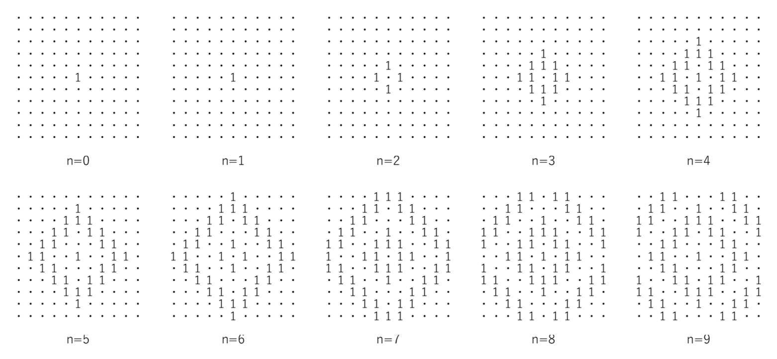
The Figure 3.2 shows a process to form a stable ‘target’ pattern. At the center, the value changes periodically as 1,1,0,0 and square-shaped waves appear and spread outwards repeatedly with period 4.
Refer to caption
Figure 3.2: Target pattern.

The Figure 3.3 shows a process to form a stable ‘spiral’ pattern. By an horizontal line of value 1, a spirals appear from its end points. Thereafter, the spirals spread through the whole space and each rotates by 90 degrees per unit time. Also, the spirals collide and disappear without any other interaction.

Refer to caption
Figure 3.3: Spiral pattern.

The behavior of these solutions is similar to that of the BZ reaction patterns.

4 Ultradiscrete two-variable Oregonator

4.1 Equilibrium points

The eq.(2.13) with (α,β)=(0,0)(\alpha,\beta)=(0,0) is the following second order ordinary difference equation:

Un+1=\displaystyle U_{n+1}= max⁡{Un,F+Q+Un−1−max⁡(Un,Q)}\displaystyle\max\{U_{n},F+Q+U_{n-1}-\max(U_{n},Q)\}
−max⁡{Un,F+Un−1−max⁡(Un,Q)},\displaystyle-\max\{U_{n},F+U_{n-1}-\max(U_{n},Q)\}, (4.1)

which can be regarded as the equation without diffusion effect. We consider the equilibrium points of the eq.(4.1).

(I) If Un≥QU_{n}\geq Q, we get

U¯={0(F+Q≤0&F≤0),Q(F≥0&F≥Q).\bar{U}=\begin{cases}0&(F+Q\leq 0\;\&\;F\leq 0),\\ Q&(F\geq 0\;\&\;F\geq Q).\end{cases} (4.2)

(II) If Un≤QU_{n}\leq Q, we get

U¯={0(F≤Q&F≤0),F(0<F<Q),Q(F≥0&F≥Q),\bar{U}=\begin{cases}0&(F\leq Q\;\&\;F\leq 0),\\ F&(0<F<Q),\\ Q&(F\geq 0\;\&\;F\geq Q),\end{cases} (4.3)

where, 0,Q0,\>Q are stable equilibrium points, and FF is an unstable equilibrium point.

4.2 Periodic solution

In this section, we suppose 0<F<Q0<F<Q and F,Q,U0,U1∈ℤF,\>Q,\>U_{0},\>U_{1}\in\mathbb{Z} in the eq.(4.1), which implies Un∈ℤU_{n}\in\mathbb{Z}. In this case, the stable equilibrium points disappear. This situaton is very similar to that of the original differential equations in which the limit cycle (oscillation) appears.

We shall obtain the solution of the eq.(4.1).

(I) When Un≥QU_{n}\geq Q, we get

Un+1={0(F+Q+Un−1−2​Un≤0),F+Q+Un−1−2​Un(F+Un−1−2​Un<0<F+Q+Un−1−2​Un),Q(F+Un−1−2​Un≥0),U_{n+1}=\begin{cases}0&(F+Q+U_{n-1}-2U_{n}\leq 0),\\ F+Q+U_{n-1}-2U_{n}&(F+U_{n-1}-2U_{n}<0<F+Q+U_{n-1}-2U_{n}),\\ Q&(F+U_{n-1}-2U_{n}\geq 0),\end{cases} (4.4)

which implies Un+1≤QU_{n+1}\leq Q. Thus, the next step is in the following case (II).

(II) When Un≤QU_{n}\leq Q, we get

Un+1={0(F+Un−1−Un≤0),F+Un−1−Un(F−Q+Un−1−Un<0<F+Un−1−Un),Q(F−Q+Un−1−Un≥0).U_{n+1}=\begin{cases}0&(F+U_{n-1}-U_{n}\leq 0),\\ F+U_{n-1}-U_{n}&(F-Q+U_{n-1}-U_{n}<0<F+U_{n-1}-U_{n}),\\ Q&(F-Q+U_{n-1}-U_{n}\geq 0).\end{cases} (4.5)

It follows that Un+1≤QU_{n+1}\leq Q. Thus, once UnU_{n} satisfies the case (II), it keeps in the case (II) all the time.

Therefore, we only consider solutions satisfying the case (II). For brevity, let Ψn=Un−1−Un\Psi_{n}=U_{n-1}-U_{n}. Eq.(4.5) can be rewritten as

Un+1={0(Ψn≤−F),F+Ψn(−F<Ψn<Q−F),Q(Ψn≥Q−F).U_{n+1}=\begin{cases}0&(\Psi_{n}\leq-F),\\ F+\Psi_{n}&(-F<\Psi_{n}<Q-F),\\ Q&(\Psi_{n}\geq Q-F).\end{cases} (4.6)

Next, we put I1=(−∞,−F],I2=(−F,Q−F),I3=[Q−F,∞)I_{1}=(-\infty,-F],\>I_{2}=(-F,Q-F),\>I_{3}=[Q-F,\infty). The combination of (Ψn,Ψn+1)(\Psi_{n},\Psi_{n+1}) can be divided into 3×33\times 3 cases.

(1-1) In the case (Ψn,Ψn+1)∈I1×I1(\Psi_{n},\Psi_{n+1})\in I_{1}\times I_{1}, we get

(Un+1,Ψn+1)\displaystyle(U_{n+1},\Psi_{n+1}) =(0,Un),\displaystyle=(0,U_{n}),
(Un+2,Ψn+2)\displaystyle(U_{n+2},\Psi_{n+2}) =(0,0),\displaystyle=(0,0),

and thus (Ψn+1,Ψn+2)∈I1×I2(\Psi_{n+1},\Psi_{n+2})\in I_{1}\times I_{2}. Therefore, the state changes from (1-1) to (1-2).

(1-2) In the case (Ψn,Ψn+1)∈I1×I2(\Psi_{n},\Psi_{n+1})\in I_{1}\times I_{2}, it follows that (Ψn+1,Ψn+2)∈I2×Ii(\Psi_{n+1},\Psi_{n+2})\in I_{2}\times I_{i} for some ii.

(1-3) In the case (Ψn,Ψn+1)∈I1×I3(\Psi_{n},\Psi_{n+1})\in I_{1}\times I_{3}, we get

(Un+1,Ψn+1)\displaystyle(U_{n+1},\Psi_{n+1}) =(0,Un),\displaystyle=(0,U_{n}),
(Un+2,Ψn+2)\displaystyle(U_{n+2},\Psi_{n+2}) =(Q,−Q),\displaystyle=(Q,-Q),
(Un+3,Ψn+3)\displaystyle(U_{n+3},\Psi_{n+3}) =(0,Q),\displaystyle=(0,Q),
(Un+4,Ψn+4)\displaystyle(U_{n+4},\Psi_{n+4}) =(Q,−Q),\displaystyle=(Q,-Q),

Therefore, UnU_{n} alternates between 00 and QQ from a certain time.

(2-1) In the case (Ψn,Ψn+1)∈I2×I1(\Psi_{n},\Psi_{n+1})\in I_{2}\times I_{1}, we get

(Un+1,Ψn+1)\displaystyle(U_{n+1},\Psi_{n+1}) =(F+Ψn,Un−(F+Ψn)),\displaystyle=(F+\Psi_{n},U_{n}-(F+\Psi_{n})),
(Un+2,Ψn+2)\displaystyle(U_{n+2},\Psi_{n+2}) =(0,F+Ψn),\displaystyle=(0,F+\Psi_{n}),

where

{Ψn+2∈I3(Ψn≥Q−2​F),Ψn+2∈I2(Ψn<Q−2​F).\begin{cases}\Psi_{n+2}\in I_{3}&(\Psi_{n}\geq Q-2F),\\ \Psi_{n+2}\in I_{2}&(\Psi_{n}<Q-2F).\end{cases}

(2-1-a) In the case Ψn≥Q−2​F\Psi_{n}\geq Q-2F, we have (Ψn+1,Ψn+2)∈I1×I3(\Psi_{n+1},\Psi_{n+2})\in I_{1}\times I_{3}.

(2-1-b) In the case Ψn<Q−2​F\Psi_{n}<Q-2F, we get

(Un+3,Ψn+3)\displaystyle(U_{n+3},\Psi_{n+3}) =(2​F+Ψn,−2​F−Ψn),\displaystyle=(2F+\Psi_{n},-2F-\Psi_{n}),
(Un+4,Ψn+4)\displaystyle(U_{n+4},\Psi_{n+4}) =(0,2​F+Ψn),\displaystyle=(0,2F+\Psi_{n}),

where

{Ψn+4∈I3(Ψn≥Q−3​F),Ψn+4∈I2(Ψn<Q−3​F).\begin{cases}\Psi_{n+4}\in I_{3}&(\Psi_{n}\geq Q-3F),\\ \Psi_{n+4}\in I_{2}&(\Psi_{n}<Q-3F).\end{cases}

(2-1-c) In the case Ψn≥Q−3​F\Psi_{n}\geq Q-3F, we have (Ψn+3,Ψn+4)∈I1×I3(\Psi_{n+3},\Psi_{n+4})\in I_{1}\times I_{3}.

(2-1-d) In the case Ψn<Q−3​F\Psi_{n}<Q-3F, repeat the above operation.

If the above discussion did not stop, Ψn+i∉I3\Psi_{n+i}\notin I_{3} would be satisfied all the time. That means Ψn<Q−m​F​(m≥2)\Psi_{n}<Q-mF\>\>(m\geq 2), which contradicts −F<Ψn<Q−F-F<\Psi_{n}<Q-F. Therefore, (Ψn′,Ψn′+1)∈I1×I3(\Psi_{n^{\prime}},\Psi_{n^{\prime}+1})\in I_{1}\times I_{3} is satisfied for a certain n′n^{\prime}.

(2-2) In the case (Ψn,Ψn+1)∈I2×I2(\Psi_{n},\Psi_{n+1})\in I_{2}\times I_{2}, it follows that (Ψn+1,Ψn+2)∈I2×Ii(\Psi_{n+1},\Psi_{n+2})\in I_{2}\times I_{i} for some ii. If we consider the case of continuing to meet (Ψn,Ψn+1)∈I2×I2(\Psi_{n},\Psi_{n+1})\in I_{2}\times I_{2}, we get

Ψn+2=Ψn−Ψn+1.\Psi_{n+2}=\Psi_{n}-\Psi_{n+1}. (4.7)

The general solution is

Ψn=\displaystyle\Psi_{n}= (−1)n−1​c1​(1+52)n−1+c2​(−1+52)n−1,\displaystyle(-1)^{n-1}c_{1}\left(\frac{1+\sqrt{5}}{2}\right)^{n-1}+c_{2}\left(\frac{-1+\sqrt{5}}{2}\right)^{n-1}, (4.8)

where

c1=Ψ2−(−1+52)​Ψ1,c2=Ψ2+(1+52)​Ψ1.c_{1}=\Psi_{2}-\left(\frac{-1+\sqrt{5}}{2}\right)\Psi_{1},\>c_{2}=\Psi_{2}+\left(\frac{1+\sqrt{5}}{2}\right)\Psi_{1}.

We easily find c1=0⇔Ψ1=Ψ2=0c_{1}=0\Leftrightarrow\Psi_{1}=\Psi_{2}=0 by Un∈ℤU_{n}\in\mathbb{Z}.

(2-2-a) In the case (Ψ1,Ψ2)≠(0,0)(\Psi_{1},\Psi_{2})\neq(0,0), taking the limit n→∞n\rightarrow\infty, absolute value of Ψn\Psi_{n} diverges to infinity. Therefore, (Ψn′,Ψn′+1)∈I2×Ii​(i=1,3)(\Psi_{n^{\prime}},\Psi_{n^{\prime}+1})\in I_{2}\times I_{i}\>(i=1,3) is satisfied for a certain n′n^{\prime}.

(2-2-b) In the case (Ψ1,Ψ2)=(0,0)(\Psi_{1},\Psi_{2})=(0,0), we get (U0,U1)=(F,F)(U_{0},U_{1})=(F,F). Then, we obtain Un=FU_{n}=F for all nn.

(2-3) In the case (Ψn,Ψn+1)∈I2×I3(\Psi_{n},\Psi_{n+1})\in I_{2}\times I_{3}, we get

(Un+1,Ψn+1)\displaystyle(U_{n+1},\Psi_{n+1}) =(F+Ψn,Un−(F+Ψn)),\displaystyle=(F+\Psi_{n},U_{n}-(F+\Psi_{n})),
(Un+2,Ψn+2)\displaystyle(U_{n+2},\Psi_{n+2}) =(Q,Ψn−(Q−F)),\displaystyle=(Q,\Psi_{n}-(Q-F)),

where

{Ψn+2∈I1(Ψn≤(Q−F)−F),Ψn+2∈I2(Ψn>(Q−F)−F).\begin{cases}\Psi_{n+2}\in I_{1}&(\Psi_{n}\leq(Q-F)-F),\\ \Psi_{n+2}\in I_{2}&(\Psi_{n}>(Q-F)-F).\end{cases}

(2-3-a) In the case Ψn≤(Q−F)−F\Psi_{n}\leq(Q-F)-F, we have (Ψn+1,Ψn+2)∈I3×I1(\Psi_{n+1},\Psi_{n+2})\in I_{3}\times I_{1}.

(2-3-b) In the case Ψn>(Q−F)−F\Psi_{n}>(Q-F)-F, we get

(Un+3,Ψn+3)\displaystyle(U_{n+3},\Psi_{n+3}) =(F+Ψn−(Q−F),−Ψn+2​(Q−F)),\displaystyle=(F+\Psi_{n}-(Q-F),-\Psi_{n}+2(Q-F)),
(Un+4,Ψn+4)\displaystyle(U_{n+4},\Psi_{n+4}) =(Q,Ψn−2​(Q−F)),\displaystyle=(Q,\Psi_{n}-2(Q-F)),

where

{Ψn+4∈I1(Ψn≤2​(Q−F)−F),Ψn+4∈I2(Ψn>2​(Q−F)−F).\begin{cases}\Psi_{n+4}\in I_{1}&(\Psi_{n}\leq 2(Q-F)-F),\\ \Psi_{n+4}\in I_{2}&(\Psi_{n}>2(Q-F)-F).\end{cases}

(2-3-c) In the case Ψn≤2​(Q−F)−F\Psi_{n}\leq 2(Q-F)-F, we have (Ψn+3,Ψn+4)∈I3×I1(\Psi_{n+3},\Psi_{n+4})\in I_{3}\times I_{1}.

(2-3-d) In the case Ψn>2​(Q−F)−F\Psi_{n}>2(Q-F)-F, repeat the above operation.

If the above discussion did not stop, Ψn+i∉I1\Psi_{n+i}\notin I_{1} would be satisfied all the time. It means Ψn<m⁡(Q−F)−F⁡(m≥1)\Psi_{n}<m(Q-F)-F\>\>(m\geq 1), which contradicts −F<Ψn<Q−F-F<\Psi_{n}<Q-F. Therefore, (Ψn′,Ψn′+1)∈I3×I1(\Psi_{n^{\prime}},\Psi_{n^{\prime}+1})\in I_{3}\times I_{1} is satisfied for a certain n′n^{\prime}.

(3-1) In the case (Ψn,Ψn+1)∈I3×I1(\Psi_{n},\Psi_{n+1})\in I_{3}\times I_{1}, we get

(Un+1,Ψn+1)\displaystyle(U_{n+1},\Psi_{n+1}) =(Q,Un−Q),\displaystyle=(Q,U_{n}-Q),
(Un+2,Ψn+2)\displaystyle(U_{n+2},\Psi_{n+2}) =(0,Q),\displaystyle=(0,Q),
(Un+3,Ψn+3)\displaystyle(U_{n+3},\Psi_{n+3}) =(Q,−Q),\displaystyle=(Q,-Q),
(Un+4,Ψn+4)\displaystyle(U_{n+4},\Psi_{n+4}) =(0,Q),\displaystyle=(0,Q),

Therefore, UnU_{n} alternates between 00 and QQ from a certain time.

(3-2) In the case (Ψn,Ψn+1)∈I3×I2(\Psi_{n},\Psi_{n+1})\in I_{3}\times I_{2}, it follows that (Ψn+1,Ψn+2)∈I2×Ii(\Psi_{n+1},\Psi_{n+2})\in I_{2}\times I_{i} for some ii.

(3-3) In the case (Ψn,Ψn+1)∈I3×I3(\Psi_{n},\Psi_{n+1})\in I_{3}\times I_{3}, we get

(Un+1,Ψn+1)\displaystyle(U_{n+1},\Psi_{n+1}) =(Q,Un−Q),\displaystyle=(Q,U_{n}-Q),
(Un+2,Ψn+2)\displaystyle(U_{n+2},\Psi_{n+2}) =(Q,0),\displaystyle=(Q,0),

and thus (Ψn+1,Ψn+2)∈I3×I2(\Psi_{n+1},\Psi_{n+2})\in I_{3}\times I_{2}.

From the above, a solution of the ultradiscrete equation (4.1) settles to the periodic solution (0,Q,0,Q,…)(0,Q,0,Q,\ldots) except for the stationary solution FF. It is can be considered that the periodic solution (0,Q,0,Q,…)(0,Q,0,Q,\ldots) corresponds to the limit cycle (oscillation) in the original differential equations. The stationary solution FF is unstable equilibrium points.

Acknowledgment

The author thanks Prof. Seiji Nishioka of Yamagata University for his invaluable advice.

References

  • [1] M. Murata “Tropical discretization: ultradiscrete Fisher-KPP equation and ultradiscrete Allen-cahn equation,” J. differ. Equ. Appl., 19 (2013), 1008–1021.
  • [2] K. Matsuya and M. Murata “Spatial pattern of discrete and ultradiscrete Gray-Scott model,” Discrete Contin. Dyn. Syst. Ser. B, 20 (2015), 173–187.
  • [3] D. Takahashi, A. Shida and M. Usami “On the pattern formation mechanism of (2+1)D max-plus models,” J. Phys. A: Math. Gen., 34 (2001), 10715–10726.
  • [4] R. Hirota and D. Takahashi “Difference and ultradiscrete systems,” Kyoritsu Shuppan, 2015.
  • [5] J. H. Merkin “On wave trains arising in the two-variable Oregonator model for the BZ reaction,” IMA. J. Appl. Math., 78 (2013), 513–536.