Analysis of Distributed ADMM Algorithm for Consensus Optimization in Presence of Node Error

In the advent of big data, the Internet of Things and cyber-physical systems, distributed processing algorithms have attracted increasing research attention. Considerable problems in these areas including network flow control, feature extraction and power system state estimation, are formulated as convex optimization problems, and use distributed optimization methods [2]-[9]. These algorithms may be characterized by their range of applicability, convergence behavior, performance, and computational complexity.

Alternating Direction Method of Multipliers (ADMM) is one of the popular convex optimization algorithms which can be implemented in a distributed manner. Wide range of applicability and convergence with an adequate accuracy within a few tens of iterations make ADMM very useful in practice. Different applications and convergence behavior of ADMM algorithm are discussed in [10] - [20]. An upper bound on the global linear convergence rate of ADMM algorithm for strongly convex objective function under smoothness assumptions is provided in [20]. A parameter selection method which optimizes the derived convergence bound is also presented in this work.

Decentralized consensus optimization is an important family of optimization problems which is formulated as

where $\tilde{\textbf{x}}\in\mathbb{R}^{n}$ and $f_{i}(\tilde{\mathbf{x}}):\mathbb{R}^{n}\rightarrow\mathbb{R}$ are convex functions. $N$ agents aim to optimize the sum of local objective functions, $f_{i}(\tilde{\mathbf{x}}),i\in\{1,...,N\}$, over a global variable $\tilde{\mathbf{x}}$. Distributed ADMM-based algorithms for consensus optimization problems can be classified into two categories. In the first one, there is a central collector or fusion center that all agents communicate with. Indeed the agents and the fusion center form a star network [10]. In the second one, there is not a fusion center, and the underlying network between the agents can have any connected topology  [21]-[24]. While the former category has better convergence rate, the flexibility of network topology in the latter one is more appealing. A framework is provided in [25], which improves the convergence property of the latter category by allowing multiple fusion centers in the network.

The distributed optimization algorithms rely on local computations and communication between neighbors. They potentially suffer from different types of errors and imperfections such as computation, quantization and communication errors and link failure which could substantially affect the performance of distributed optimization methods. The subgradient-push algorithm which is convergent over time varying networks is proposed in [26]. ADMM-based algorithms which are resilient to link failure are proposed in [27]. Certain local computations are too complex to be carried out exactly and are usually replaced by approximations. Inexact variants of ADMM algorithm are proposed in [21, 28, 29, 30]. In [21], three distributed ADMM-based algorithms are proposed to solve the Lasso problem offering different computational complexity and convergence rate trade-offs. In [28] each ADMM update step, which includes solving an optimization subproblem, is replaced by an inexact step which reduces the computational cost of the algorithm by an order of magnitude. In [29] and [30], the Lagrangian minimization in each ADMM step is, respectively, replaced by linear and quadratic approximations of the objective function. The quadratic approximation is more complex than the linear approximation, but results in an algorithm with better convergence properties. A distributed subgradient method for consensus optimization which is convergent in presence of quantization error is proposed in [31]. In [32], ADMM-based distributed algorithms are proposed for parameter estimation in ad hoc wireless sensor networks which exhibit resilience in the presence of communication/quantization noise. For the least square objective function, the steady state error of the algorithm is analyzed. A robust ADMM-based distributed algorithm for average consensus problem in presence of noise is presented in [33].

In this work, we focus on analyzing the convergence behavior of distributed ADMM for consensus optimization over a connected network in presence of additive node error. We consider general convex or strongly convex local objective functions. In this setting, the latest estimate of the solution computed at each node is subject to additive random noise prior to transmission to neighboring nodes (this for instance could be due to quantization error [34]). We provide analytical upper and lower bounds on the mean squared steady state error of the noisy ADMM algorithm for consensus, when local objective functions are strongly convex and have Lipschitz continuous gradients. In addition, we show that for convex, proper and closed local objective functions and in presence of bounded node error, the steady state error of noisy ADMM algorithm for consensus is bounded. Extensive numerical results are provided which shows the effectiveness of the presented analyses. We also study the effect of different factors, such as noise variance, network topology and ADMM algorithm parameter on the provided bounds. We also propose a method to tune the algorithm parameter, which results in a faster convergence rate and a smaller steady state error.

The rest of the paper is organized as follows. The system model and prior art is reviewed in good details in Section II. Section III analyzes the convergence behavior of the algorithm in presence of additive node error. Analytical results are numerically assessed in Section IV, and conclusions are drawn in Section V.

Consider a set of $N$ nodes that intend to solve the consensus optimization problem in (1) in a distributed manner and over a given connected network with $E$ undirected links. The network can be represented by the graph $\mathcal{G}=(\mathcal{V},\mathcal{A})$, where $\mathcal{V}$ is the set of nodes, $|\mathcal{V}|=N$, and $\mathcal{A}$ is the set of arcs, $|\mathcal{A}|=2E$. Communications of nodes are synchronous and restricted to the neighbors.

It is shown that with the following assumption, the proposed algorithm converges R-linearly to its optimal point over a fixed connected underlying network[24].

According to Assumption 1, $f(\mathbf{x})$ is a strongly convex function with module $m_{f}=\min_{i}m_{f_{i}}$ and its gradient is Lipschitz continuous with constant $M_{f}=\max_{i}M_{f_{i}}$.

In this section, we consider the scenario where the neighboring nodes only exchange a noisy version of their messages in Step 2 of Algorithm 1. We model the node error $\mathbf{e}_{x,i}^{k}$ at node $i$ in iteration $k$, as zero mean, additive and independent, identically distributed (i.i.d) error. We have

where $\hat{\mathbf{x}}_{i}^{k}$ is the message that node $i\in\mathcal{N}$ communicates to its neighbors at iteration $k$; and $\hat{\mathbf{x}}\in\mathbb{R}^{nN}$ and $\mathbf{e}_{x}^{k}\in\mathbb{R}^{nN}$ denote the concatenated versions of $\hat{\mathbf{x}}_{i}^{k}$ and $\mathbf{e}_{x,i}^{k}$ for all $i$.

The noisy ADMM algorithm can be derived by replacing $\mathbf{x}^{k+1}$ with $\hat{\mathbf{x}}^{k+1}$ in (4b) and (4c). We have

Note that $\hat{\mathbf{x}}^{k+1}$, $\hat{\mathbf{z}}^{k+1}$ and $\hat{\boldsymbol{\lambda}}^{k+1}$ represent the variables affected by node noise $\mathbf{e}_{x}^{k+1}$. Considering $\hat{\boldsymbol{\lambda}}=[\hat{\boldsymbol{\beta}};\hat{\boldsymbol{\nu}}]$ with $\hat{\boldsymbol{\beta}},\hat{\boldsymbol{\nu}}\in\mathbb{R}^{2nE}$, and letting $\mathbf{z}^{k+1}=\frac{1}{2}\mathbf{M}_{+}^{T}\mathbf{x}^{k+1}$ and $\boldsymbol{\beta}^{k+1}=\hat{\boldsymbol{\beta}}^{k}+\frac{c}{2}\mathbf{M}_{-}^{T}\mathbf{x}^{k+1}$, with some mathematical manipulations similar to those done in the derivation of (5), we have

which can be considered as the noisy version of iteration in (5). With some algebraic manipulations, this iteration results in the distributed noisy ADMM algorithm outlined in Algorithm 2.

In the following theorem we analyze the convergence behavior of $d^{k}$ where

and

and $\mathbf{u}^{*}$ and $\mathbf{G}$ are defined in (8). From (18) it can be seen that $d^{k}$ is a random variable, whose randomness is caused by error sequence $\{\mathbf{e}_{x}^{1},\dots,\mathbf{e}_{x}^{k}\}$. In Theorem 2, we obtain an upper bound on $\underset{k\rightarrow\infty}{\operatorname{lim}}\mathbb{E}[d^{k}]$, which shows that $\underset{k\rightarrow\infty}{\lim}\hskip 2.84526ptd^{k}$ is bounded. As we shall demonstrate in proof of this theorem, boundedness of $\underset{k\rightarrow\infty}{\lim}\hskip 2.84526ptd^{k}$ dictates that $\underset{k\rightarrow\infty}{\lim}\hskip 2.84526pt\|\mathbf{x}^{k}-\mathbf{x}^{*}\|_{2}^{2}$ is finite. We provide an upper bound on the mean squared steady state error $\underset{k\rightarrow\infty}{\operatorname{lim}}\mathbb{E}[\|\mathbf{x}^{k+1}-\mathbf{x}^{*}\|_{2}^{2}]$ of the algorithm. The proof of the theorem requires the KKT conditions for (3) to hold, i.e.,

In this section, we use Algorithm 2 to solve the following optimization problem

$N$ agents estimate variable $\tilde{\mathbf{x}}$ using noisy linear observations $\mathbf{y}_{i}=\mathbf{M}_{i}\tilde{\mathbf{x}}+\mathbf{n}_{i}$, cooperatively. The variables communicated between neighbors are subject to additive node error as in (16). In these experiments, the elements of error vector are i.i.d and follow uniform distribution $\mathcal{U}(-\epsilon,\epsilon)$. We consider network edge density as $r\triangleq\frac{E}{E_{c}}$, where $E_{c}$ is the number of edges in a corresponding complete graph. Consider $\mathbf{x}_{k}^{D}$ and $\mathbf{x}^{C}$ as respectively the distributed and centralized estimates of $\mathbf{x}$ (at iteration $k$). Our performance metrics are the relative error $\sqrt{\mathbb{E}[\mathcal{E}^{DC}_{k}]}$, where $\mathcal{E}^{DC}_{k}=\frac{\|\mathbf{x}^{D}_{k}-\mathbf{x}^{C}\|_{2}^{2}}{\|\mathbf{x}^{C}\|_{2}^{2}}$, and steady state error $\underset{k\rightarrow\infty}{\operatorname{lim}}\sqrt{\mathbb{E}[\mathcal{E}^{DC}_{k}]}$.

In the first set of experiments, the number of agents $N$ is $20$, and $\tilde{\mathbf{x}}\in\mathbb{R}^{20}$ (i.e., $n=20$) and its elements are i.i.d from $\mathcal{N}(0,1)$. Measurement matrices $\mathbf{M}_{i}\in\mathbb{R}^{5\times 20}$, which means that local objective functions are not strongly convex. The observation noise is $\mathbf{n}_{i}\sim\mathcal{N}(\mathbf{0},\sigma^{2}\mathbf{I}_{5})$ and $\sigma^{2}=0.1$. Figure 1 presents the relative error of the algorithm as a function of iteration index $k$ for different values of $\epsilon$. In this experiment $c=1$ and $r=0.5$. As evident the algorithm is convergent, which confirms theoretical result form Theorem 4.

In the second set of experiments the local objective functions satisfy Assumption 1, and $\tilde{\mathbf{x}}\in\mathbb{R}^{3}$ (i.e., $n=3$) and its elements are i.i.d from $\mathcal{N}(0,1)$. We first generate measurement matrices $\mathbf{M}_{i}\in\mathbb{R}^{3\times 3}$, whose elements are i.i.d from $\mathcal{N}(0,1)$. Then, scale their singular values to the range $[\sqrt{m_{f}},\sqrt{M_{f}}]$ and rebuild $\mathbf{M}_{i}$. The observation noise is $\mathbf{n}_{i}\sim\mathcal{N}(\mathbf{0},\sigma^{2}\mathbf{I}_{3})$ and $\sigma^{2}=0.1$. In the following experiments, unless otherwise stated, the parameter $c$ is set to $c^{*}$ in (14).

The upper bound in Theorem 2 depends on $\delta$ whose theoretical value is presented in (11). In numerical experiments, we can compute this parameter by estimating convergence rate of the algorithm experimentally. Define $\rho_{e}^{k}$ as the estimated convergence rate of the algorithm at iteration $k$

The geometric average rate of convergence of the algorithm is

Based on (11) and (31), we have

In the sequel, the upper bounds in Theorem 2 which are computed based on different $\delta$ parameters presented in (11) and (32) are referred to as theoretical upper bound, $\text{UB}_{t}$, and experimental upper bound, $\text{UB}_{e}$, respectively. The lower bound in Theorem 3 is labeled as LB.

Figure 2 depicts the relative error of Algorithm 2 as a function of iteration number $k$. In this experiment, the nodes communicate over a randomly generated connected network of $N=20$ nodes with edge density $0.5$, and $\epsilon=10^{-4}$. The performance of the algorithm in error free scenario is also presented for comparison. As seen, $\text{UB}_{e}$ is a tighter bound than $\text{UB}_{t}$, indicating that experimentally computed convergence rate is more accurate.

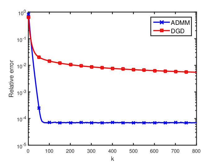
A distributed subgradient method is proposed in [31], which is convergent in presence of quantization error. Figure 3 presents the performance of this algorithm, labeled as DGD and Algorithm 2 (ADMM), for comparison. In this experiment, we have $N=20$ and $r=0.5$. This figure shows that the ADMM-based algorithm outperforms DGD algorithm.

Figure 4 shows the effect of $\epsilon$ on steady state error of Algorithm 2. In the current experiment set up with the least squares as the objective function of the optimization problem, one can show that indeed the steady state error of the algorithm is a linear function of the node error. This holds true not only in the performance of the algorithm (as reflected in simulations), but also in the presented lower and upper bounds.

Figure 5 presents the influence of network edge density on the steady state error of the algorithm. In this experiment networks of $N=20$ and $N=100$ nodes are generated randomly. One sees that increase in network edge density leads to little decrease in steady state error. The trends of simulation results and lower and upper bounds are consistent.

We study the performance of the noisy ADMM algorithm over regular networks as an especial case. Figure 6 depicts the effect of node degree on the steady state error of the algorithm for networks of $N=100$ nodes. As evident, the slop of the curve is a decreasing function of node degree, and varying node degree in the range of $[30\hskip 2.84544pt99]$ does not improve steady state error significantly. The upper bounds which are functions of $E$ and $\delta$, predict this behavior properly. The lower bound is just a function of $E$, and does not predict the slop of steady state error curve.

We consider tree network as another especial case. Figure 7 demonstrates the influence of branch factor parameter of the tree network on steady state error of the algorithm. It can be seen that experimental upper bound predicts the performance of the algorithm better than the other bounds, and proposed theoretical upper bound is an acceptable indicator of the algorithm behavior. From the last three sets of experiments, we can conclude that the upper bounds can predict effects of network topology on the steady state error more accurately.

Another parameter which affects the performance of the algorithm is $c$. Figure 8 shows the effect of $c$ parameter on the steady state error over the randomly generated networks. The connectivity ratio in $N=20$ and $N=100$ scenarios are $0.5$ and $0.2$, respectively. One sees that, a lower $c$ results in a lower steady state error which is also predicted by the proposed lower and experimental upper bounds. The mismatch between theoretical upper bound and simulation shows that the effect of $c$ on the convergence rate of the algorithm is not predicted properly by (10).

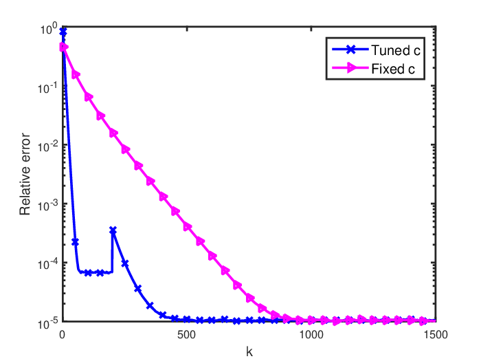
As discussed, the convergence rate and steady state error of the algorithm output depends on parameter $c$. The value of the parameter $c$ is to be selected for minimized steady state error and maximized convergence rate. According to our observations, the performance of the noisy ADMM algorithm in early iterations is similar to the noiseless case. A smaller value of $c$ results in a smaller steady state error, but it does not necessarily lead to a high convergence rate. A reasonable tuning policy is to set parameter $c$ to accelerate the convergence in early iterations, and then to reduce the parameter to aim for a small steady state error. Figure 9 depicts the performance of this tuning method. In this experiment, parameter $c$ is set to $c^{*}$ provided in (14) in the first $200$ iterations, and then it is reduced by a factor of $0.01$. The performance of the algorithm with fixed parameter $c$ set to $0.01c^{*}$ is also presented for comparison. The results confirm faster convergence rate and improved steady state error when the proposed tuning policy is in effect.

We also examined the effects of $M_{f}$, Lipschitz constant, and $m_{f}$, strong convexity module, on the steady state error of the algorithm (not reported here). We observed that the influence of these parameters is accurately predicted by the proposed lower and experimental upper bounds. The theoretical upper bound, however, does not reflect the effects of these parameters properly.

We analyzed the effect of additive node error on the performance of distributed ADMM algorithm for consensus optimization over a connected network. Analytical upper and lower bounds were provided on the mean squared steady state error of the algorithm, in the case that local objective functions are strongly convex and have Lipschitz continuous gradients. The analysis quantifies how the provided bounds depend on different factors such as noise variance and network topology. To accelerate the algorithm and also reduce the steady state error, a method was proposed to tune the algorithm parameter. In addition, it was shown that if the local objective functions are proper, closed and convex, for a bounded and random node error, the steady state error of the noisy ADMM algorithm for consensus is bounded. Numerical results validated the theoretical analyses and demonstrated the role of different system and network parameters. Analysis of the algorithm convergence behavior over the networks whose links suffer from additive noise can be considered as an important next research steps.

References

• [1] L. Majzoobi and F. Lahouti, “Analysis of distributed admm algorithm for consensus optimization in presence of error,” in 41st IEEE International Conference on Acoustics, Speech and Signal Processing (ICASSP), 2016, pp. 4831–4835.
• [2] S. H. Low and D. E. Lapsley, “Optimization flow control-I: basic algorithm and convergence,” IEEE/ACM Transactions on Networking, vol. 7, no. 6, pp. 861–874, 1999.
• [3] T. Erseghe, “Distributed optimal power flow using admm,” IEEE transactions on power systems, vol. 29, no. 5, pp. 2370–2380, 2014.
• [4] M. Rabbat and R. Nowak, “Distributed optimization in sensor networks,” in ACM Proceedings of the 3rd international symposium on Information processing in sensor networks, 2004, pp. 20–27.
• [5] A. Nedić and A. Ozdaglar, “Distributed subgradient methods for multi-agent optimization,” IEEE Transactions on Automatic Control, vol. 54, no. 1, pp. 48–61, 2009.
• [6] B. Johansson, M. Rabi, and M. Johansson, “A randomized incremental subgradient method for distributed optimization in networked systems,” SIAM Journal on Optimization, vol. 20, no. 3, pp. 1157–1170, 2009.
• [7] E. Ghadimi, I. Shames, and M. Johansson, “Multi-step gradient methods for networked optimization,” IEEE Transactions on Signal Processing, vol. 61, no. 21, pp. 5417–5429, 2013.
• [8] N. Li, “Distributed optimization in power networks and general multi-agent systems,” Ph.D. dissertation, California Institute of Technology, 2013.
• [9] T.-H. Chang, A. Nedic, and A. Scaglione, “Distributed constrained optimization by consensus-based primal-dual perturbation method,” IEEE Transactions on Automatic Control, vol. 59, no. 6, pp. 1524–1538, 2014.
• [10] S. Boyd, N. Parikh, E. Chu, B. Peleato, and J. Eckstein, “Distributed optimization and statistical learning via the alternating direction method of multipliers,” Foundations and Trends in Machine Learning, vol. 3, no. 1, pp. 1–122, 2011.
• [11] C. Shen, T.-H. Chang, K.-Y. Wang, Z. Qiu, and C.-Y. Chi, “Distributed robust multicell coordinated beamforming with imperfect csi: An admm approach,” IEEE Transactions on signal processing, vol. 60, no. 6, pp. 2988–3003, 2012.
• [12] F. Lin, M. Fardad, and M. R. Jovanović, “Design of optimal sparse feedback gains via the alternating direction method of multipliers,” IEEE Transactions on Automatic Control, vol. 58, no. 9, pp. 2426–2431, 2013.
• [13] J. Liu, P. Musialski, P. Wonka, and J. Ye, “Tensor completion for estimating missing values in visual data,” IEEE transactions on pattern analysis and machine intelligence, vol. 35, no. 1, pp. 208–220, 2013.
• [14] P. Danaher, P. Wang, and D. M. Witten, “The joint graphical lasso for inverse covariance estimation across multiple classes,” Journal of the Royal Statistical Society: Series B (Statistical Methodology), vol. 76, no. 2, pp. 373–397, 2014.
• [15] X. Qing, G. Hu, and X. Wang, “Robust compressed sensing with bounded and structured uncertainties,” IET Signal Processing, vol. 8, no. 7, pp. 783–791, 2014.
• [16] W. Deng and W. Yin, “On the global and linear convergence of the generalized alternating direction method of multipliers,” Journal of Scientific Computing, pp. 1–28, 2012.
• [17] B. He and X. Yuan, “On the o(1/n) convergence rate of the douglas-rachford alternating direction method,” SIAM Journal on Numerical Analysis, vol. 50, no. 2, pp. 700–709, 2012.
• [18] W. Deng, M.-J. Lai, Z. Peng, and W. Yin, “Parallel multi-block admm with o (1/k) convergence,” Journal of Scientific Computing, pp. 1–25, 2014.
• [19] T. Goldstein, B. O’Donoghue, S. Setzer, and R. Baraniuk, “Fast alternating direction optimization methods,” SIAM Journal on Imaging Sciences, vol. 7, no. 3, pp. 1588–1623, 2014.
• [20] P. Giselsson and S. Boyd, “Linear convergence and metric selection for douglas-rachford splitting and admm,” IEEE Transactions on Automatic Control, vol. 62, no. 2, pp. 532–544, 2017.
• [21] G. Mateos, J. A. Bazerque, and G. B. Giannakis, “Distributed sparse linear regression,” IEEE Transactions on Signal Processing, vol. 58, no. 10, pp. 5262–5276, 2010.
• [22] R. H. Etemad and F. Lahouti, “Resilient decentralized consensus-based state estimation for smart grid in presence of false data,” in 41st IEEE International Conference on Acoustics, Speech and Signal Processing (ICASSP), 2016, pp. 3466–3470.
• [23] J. F. Mota, J. M. Xavier, P. M. Aguiar, and M. Puschel, “D-admm: A communication-efficient distributed algorithm for separable optimization,” IEEE Transactions on Signal Processing, vol. 61, no. 10, pp. 2718–2723, 2013.
• [24] W. Shi, Q. Ling, K. Yuan, G. Wu, and W. Yin, “On the linear convergence of the admm in decentralized consensus optimization,” IEEE Transactions on Signal Processing, vol. 62, no. 7, pp. 1750–1761, 2014.
• [25] M. Ma, A. N. Nikolakopoulos, and G. B. Giannakis, “Fast decentralized learning via hybrid consensus admm,” in IEEE International Conference on Acoustics, Speech and Signal Processing (ICASSP), Calgary, Alberta, Canada, 2018.
• [26] A. Nedić and A. Olshevsky, “Distributed optimization over time-varying directed graphs,” IEEE Transactions on Automatic Control, vol. 60, no. 3, pp. 601–615, 2015.
• [27] L. Majzoobi, V. Shah-Mansouri, and F. Lahouti, “Analysis of distributed admm algorithm for consensus optimisation over lossy networks,” IET Signal Processing, vol. 12, no. 6, pp. 786–794, 2018.
• [28] T.-H. Chang, M. Hong, and X. Wang, “Multi-agent distributed optimization via inexact consensus admm,” IEEE Transactions on Signal Processing, vol. 63, no. 2, pp. 482–497, 2015.
• [29] Q. Ling, W. Shi, G. Wu, and A. Ribeiro, “Dlm: Decentralized linearized alternating direction method of multipliers.” IEEE Transactions Signal Processing, vol. 63, no. 15, pp. 4051–4064, 2015.
• [30] A. Mokhtari, W. Shi, Q. Ling, and A. Ribeiro, “Decentralized quadratically approximated alternating direction method of multipliers,” in IEEE Global Conference on Signal and Information Processing (GlobalSIP), 2015, pp. 795–799.
• [31] A. Nedic, A. Olshevsky, A. Ozdaglar, and J. N. Tsitsiklis, “Distributed subgradient methods and quantization effects,” in IEEE 47th Conference on Decision and Control (CDC), 2008, pp. 4177–4184.
• [32] I. D. Schizas, A. Ribeiro, and G. B. Giannakis, “Consensus in ad hoc wsns with noisy links—part i: Distributed estimation of deterministic signals,” IEEE Transactions on Signal Processing, vol. 56, no. 1, pp. 350–364, 2008.
• [33] T. Erseghe, D. Zennaro, E. Dall’Anese, and L. Vangelista, “Fast consensus by the alternating direction multipliers method,” IEEE Transactions on Signal Processing, vol. 59, no. 11, pp. 5523–5537, 2011.
• [34] D. Marco and D. L. Neuhoff, “The validity of the additive noise model for uniform scalar quantizers,” IEEE Transactions on Information Theory, vol. 51, no. 5, pp. 1739–1755, 2005.