We construct a gauge-invariant action for open superstring field theory up to quartic order including the Ramond sector based on the covering of the supermoduli space of super-Riemann surfaces, following the approach presented by Ohmori and Okawa. Since our approach is based on the covering of the supermoduli space, the resulting action naturally has an $A_{\infty}$ structure. In our construction, adding stubs to the star product can be easily incorporated, and we explicitly construct an action for open superstring field theory including the Ramond sector with stubs up to quartic interactions.

1 Introduction

String field theory is one approach to non-perturbative formulations of string theory. A famous example of string field theory is open bosonic string field theory by Witten [1]. Its action has a Chern-Simons-like gauge invariance. One of the achievements in open bosonic string field theory is the construction of the analytic solution for the tachyon vacuum by Schnabl [2]. If we are interested in quantum aspects of string field theory, however, bosonic string field theory suffers from vacuum instability caused by tachyon fields, and it is desirable to consider superstring field theory.

One of the successful constructions of an action for the Neveu-Schwarz sector of open superstring field theory was presented by Berkovits [3]. The key ingredient of this formulation is use of the large Hilbert space of the superconformal ghost [4]. The fundamental string field is in the large Hilbert space, and the action is written in a closed form, realizing a Wess-Zumino-Witten-like gauge invariance. However, its gauge fixing turned out to be very difficult. On the other hand, it is known that the gauge-fixing by the Batalin-Vilkovisky formalism is straightforward if an action has a structure called cyclic $A_{\infty}$ , and an action for the Neveu-Schwarz sector of open superstring field theory with a cyclic $A_{\infty}$ structure was constructed by Erler, Konopka, and Sachs [5]. A set of multi-string products with the $A_{\infty}$ relations is constructed in a recursive manner, and the action is not given in a closed form. Although these two actions [3, 5] are different in appearance, it was proved that they are equivalent under partial gauge fixing and field redefinition [6, 7, 8].

Recently, a complete action for open superstring field theory including the Ramond sector was constructed by Kunitomo and Okawa in [9], extending the Wess-Zumino-Witten-like action for the Neveu-Schwarz sector [3]. Furthermore, Kunitomo, Okawa, Sukeno, and the author showed that the Feynman rules derived from this action correctly reproduce on-shell four-point and five-point amplitudes involving fermions at the tree level [10]. On the other hand, a complete action for open superstring field theory with the cyclic $A_{\infty}$ structure including the Ramond sector was constructed [11, 12], extending the action for the Neveu-Schwarz sector of open superstring field theory [5]. Although these two complete actions are different in appearance, it was proved that they are equivalent under partial gauge fixing and field redifinition [11].

In the formulations [9, 11, 12], the Ramond string field is in the restricted subspace, which preserves the BRST cohomology of the original Hilbert space of the Ramond sector. As we will explain later, the restriction on the Ramond string field is closely related to the supermoduli space of super-Riemann surfaces. Another approach to incorporate the Ramond sector in a covariant manner is to use an unrestricted Ramond string field and spurious free fields, and an action for closed superstring field theory is constructed by Sen [13]. The approach by Sen can be applied to open superstring field theory.¹¹ 1 The calculations in [10] can be also interpreted as those for the formulation [13].

In the formulations of open superstring field theory which we mentioned so far, the use of the large Hilbert space played an important role. In the Wess-Zumino-Witten-like formulation, the fundamental Neveu-Schwarz string field is in the large Hilbert space. In the recursive construction of an action with the cyclic $A_{\infty}$ structure in [5], although its fundamental string field is in the small Hilbert space, the large Hilbert space is used in intermediate steps of the construction of multi-string products. However, the use of the large Hilbert space obscures the relation between gauge invariance and the covering of the supermoduli space. To improve the understanding of the relation between them, it would be useful to construct open superstring field theory without using the large Hilbert space. Recently, a new approach to formulating open superstring field theory based on the covering of the supermoduli space of super-Riemann surfaces was proposed by Ohmori and Okawa [14]. They explicitly constructed a gauge-invariant action in the Neveu-Schwarz sector up to quartic interactions. Since their approach is based on the covering of the supermoduli space, the resulting action naturally has an $A_{\infty}$ structure.

In this paper, we extend the approach presented in [14] and construct a gauge-invariant action for open superstring field theory based on the supermoduli space including the Ramond sector up to quartic interactions. Since our approach is based on the covering of the supermoduli space, our action also has an $A_{\infty}$ structure. In our construction, adding stubs to the star product is easily incorporated, and we explicitly construct an action for open superstring field theory including the Ramond sector with stubs up to quartic interactions.

2 Open bosonic string field theory

In this section, we review open bosonic string field theory. After describing the cyclic $A_{\infty}$ structure and the extended BRST formalism, we illustrate the construction of an action of open bosonic string field theory with stubs based on the method presented in [14].

2.1 Cyclic $A_{\infty}$ structure in open bosonic string field theory

The action of open bosonic string field theory by Witten [1] is given by

S={}-\frac{1}{2}\langle\,\Psi,Q\Psi\,\rangle{}-\frac{g}{3}\langle\,\Psi,\Psi\ast\Psi\,\rangle\,,

(2.1)

where the open bosonic string field $\Psi$ is a state in the Hilbert space of the boundary CFT, $Q$ is the BRST operator, and $A\ast B$ is the star product of string fields $A$ and $B$ . The string field $\Psi$ is a Grassmann-odd state carrying the ghost number $1$ . The BRST operator $Q$ and the star product satisfy the following equations:²² 2 Here and in what follows, a state in the exponent of $-1$ represents its Grassmann parity: it is 0 mod 2 for a Grassmann-even state and 1 mod 2 for a Grassmann-odd state.

$\displaystyle Q^{2}A_{1}=$	$\displaystyle\ 0,$	(2.2)
$\displaystyle Q(A_{1}\ast A_{2})=$	$\displaystyle\ QA_{1}\ast A_{2}+(-1)^{A_{1}}A_{1}\ast QA_{2}\,,$	(2.3)
$\displaystyle(A_{1}\ast A_{2})\ast A_{3}=$	$\displaystyle\ A_{1}\ast(A_{2}\ast A_{3})\,.$	(2.4)

The action (2.1) is invariant under the following gauge transformation:

\delta\Psi=Q\Lambda-g\Lambda\ast\Psi+g\Psi\ast\Lambda\,,

(2.5)

where $\Lambda$ is the gauge parameter. The string field $\Lambda$ is a Grassmann-even state of ghost number 0. In the proof of gauge invariance, we use the equations

$\displaystyle\langle\,A_{1},A_{2}\,\rangle=$	$\displaystyle\ (-1)^{A_{1}A_{2}}\langle\,A_{2},A_{1}\,\rangle\,,$	(2.6)
$\displaystyle\langle\,QA_{1},A_{2}\,\rangle=$	$\displaystyle\ {}-(-1)^{A_{1}}\langle\,A_{1},QA_{2}\,\rangle\,,$	(2.7)
$\displaystyle\langle\,A_{1}\ast A_{2},A_{3}\,\rangle=$	$\displaystyle\ \langle\,A_{1},A_{2}\ast A_{3}\,\rangle$	(2.8)

together with the equations (2.2), (2.3), and (2.4).

Gauge-invariant actions can be constructed in terms of a set of multi-string products with properties we will explain in the following. Let us consider an action of string field theory in the following form:

S={}-\frac{1}{2}\langle\,\Psi,Q\Psi\,\rangle{}-\frac{g}{3}\langle\,\Psi,V_{2}(\Psi,\Psi)\,\rangle{}-\frac{g^{2}}{4}\langle\,\Psi,V_{3}(\Psi,\Psi,\Psi)\,\rangle+\mathcal{O}(g^{3})\,.

(2.9)

The two-string product $V_{2}(A_{1},A_{2})$ is defined for two string fields $A_{1}$ and $A_{2}$ , and its Grassmann parity is

(-1)^{V_{2}(A_{1},A_{2})}=(-1)^{A_{1}+A_{2}}\,.

(2.10)

The three-string product $V_{3}(A_{1},A_{2},A_{3})$ is defined for three string fields $A_{1}$ , $A_{2}$ , and $A_{3}$ , and its Grassmann parity is

(-1)^{V_{3}(A_{1},A_{2},A_{3})}=(-1)^{A_{1}+A_{2}+A_{3}+1}\,.

(2.11)

We assume that the two-string product and the three-string product satisfy the following cyclicity equations:

	$\displaystyle\langle\,A_{1},V_{2}(A_{2},A_{3})\,\rangle=$	$\displaystyle\ \langle\,V_{2}(A_{1},A_{2}),A_{3}\,\rangle\,,$		(2.12)
	$\displaystyle\langle\,A_{1},V_{3}(A_{2},A_{3},A_{4})\,\rangle=$	$\displaystyle\ {}-(-1)^{A_{1}}\langle\,V_{3}(A_{1},A_{2},A_{3}),A_{4}\,\rangle\,,$		(2.13)

or equivalently,

	$\displaystyle\langle\,A_{1},V_{2}(A_{2},A_{3})\,\rangle=$	$\displaystyle\ (-1)^{A_{1}(A_{2}+A_{3})}\langle\,A_{2},V_{2}(A_{3},A_{1})\,\rangle\,,$		(2.14)
	$\displaystyle\langle\,A_{1},V_{3}(A_{2},A_{3},A_{4})\,\rangle=$	$\displaystyle\,{}-(-1)^{A_{1}(A_{2}+A_{3}+A_{4})}\langle\,A_{2},V_{3}(A_{3},A_{4},A_{1})\,\rangle\,.$		(2.15)

Using the cyclicity equations, the variation of the action (2.9) is given by

\delta S={}-\langle\,\delta\Psi,Q\Psi\,\rangle{}-g^{2}\langle\,\delta\Psi,V_{3}(\Psi,\Psi,\Psi)\,\rangle+\mathcal{O}(g^{3})\,.

(2.16)

The equation of motion is

0=Q\Psi+gV_{2}(\Psi,\Psi)+g^{2}V_{3}(\Psi,\Psi,\Psi)+\mathcal{O}(g^{3})\,.

(2.17)

We can show that the action (2.9) is invariant under the following gauge transformation up to $\mathcal{O}(g^{3})$ :

\begin{split}\delta\Psi=&\ Q\Lambda-gV_{2}(\Lambda,\Psi)+gV_{2}(\Psi,\Lambda)\\ &\quad-g^{2}V_{3}(\Lambda,\Psi,\Psi)+g^{2}V_{3}(\Psi,\Lambda,\Psi)-g^{2}V_{3}(\Psi,\Psi,\Lambda)+\mathcal{O}(g^{3})\,,\end{split}

(2.18)

if the BRST operator $Q$ and the multi-string products $V_{2}$ and $V_{3}$ satisfy the following equations:

$\displaystyle 0=$	$\displaystyle\ Q^{2}A_{1},$	(2.19)
$\displaystyle 0=$	$\displaystyle\ QV_{2}(A_{1},A_{2})-V_{2}(QA_{1},A_{2})-(-1)^{A_{1}}V_{2}(A_{1},QA_{2})\,,$	(2.20)
$\displaystyle 0=$	$\displaystyle\ QV_{3}(A_{1},A_{2},A_{3})+V_{3}(QA_{1},A_{2},A_{3})$
	$\displaystyle\quad+(-1)^{A_{1}}V_{3}(A_{1},QA_{2},A_{3})+(-1)^{A_{1}+A_{2}}V_{3}(A_{1},A_{2},QA_{3})$	(2.21)
	$\displaystyle\quad{}-V_{2}(V_{2}(A_{1},A_{2}),A_{3})+V_{2}(A_{1},V_{2}(A_{2},A_{3}))\,.$

These equations can be extended to higher orders, and such the equations for multi-string products are called $A_{\infty}$ relations. If an action is constructed from a set of multi-string products which satisfy the $A_{\infty}$ relations and the cyclicity equations, the action has a cyclic $A_{\infty}$ structure. Furthermore, quantization of string field theory based on the Batalin-Vilkovisky formalism is straightforward if the theory has the cyclic $A_{\infty}$ structure.

Since the star product is associative (2.4) and the BRST operator and the star product satisfy (2.3), the BRST operator and the star product satisfy the $A_{\infty}$ relations without introducing higher multi-string products $V_{3},V_{4},\cdots$ . Since the star product satisfies the cyclicity equation (2.8), the action (2.1) has the cyclic $A_{\infty}$ structure.

In open superstring field theory or open bosonic string field theory with stubs, the two-string product $V_{2}$ is not associative:

V_{2}(V_{2}(A_{1},A_{2}),A_{3})\neq\ V_{2}(A_{1},V_{2}(A_{2},A_{3}))\,.

(2.22)

We can recover the gauge-invariance at quartic order by constructing a three-string product satisfying the $A_{\infty}$ relation (2.21).

2.2 Extended BRST formalism

The extended BRST transformation introduced by Witten in [15] is useful when we construct an action for open superstring field theory. In this subsection, we explain the extended BRST formalism for the bosonic string.³³ 3 The content of this subsection is based on the paper by Ohmori and Okawa [14]. Let us consider the tree-level four string amplitude. Using the upper-half plane (UHP), the tree-level four-point amplitude is given by

\mathcal{A}=\ g^{2}\int_{0}^{1}dt\,\langle\,\Psi_{1}(0)\,b_{-1}\cdot\Psi_{2}(t)\,\Psi_{3}(1)\,\Psi_{4}(\infty)\,\rangle_{\text{UHP}}\,,

(2.23)

where $\Psi(t)=cV^{\text{matter}}(t)$ is an unintegrated vertex operator, and we used the relation

b_{-1}\cdot\Psi(t)=V^{\text{matter}}(t)\,,

(2.24)

where $b_{-1}$ is the line integral of $b$ ghost:

b_{-1}=\,\oint\,\frac{dz}{2\pi i}\,b(z)\,.

(2.25)

Using the line integral $L_{-1}$ of the energy-momentum tensor $T(z)$ :

L_{-1}=\,\oint\,\frac{dz}{2\pi i}\,T(z)\,,

(2.26)

we find

L_{-1}\cdot V^{\text{matter}}(t)=\,\partial_{t}V^{\text{matter}}(t)\,,

(2.27)

we can express this amplitude in the following form:

\mathcal{A}=\ g^{2}\int_{0}^{1}dt\,\langle\,\Psi_{1}(0)\,b_{-1}e^{tL_{-1}}\cdot\Psi_{2}(0)\,\Psi_{3}(1)\,\Psi_{4}(\infty)\,\rangle_{\text{UHP}}\,.

(2.28)

Following [15], We introduce a Grassmann-odd parameter $\tilde{t}$ . Our convention for the integral over the Grassmann-odd variable is

\int d\tilde{t}\,\tilde{t}=1\,.

(2.29)

Then we can write the four-string amplitude as

\mathcal{A}={}-\,g^{2}\int_{0}^{1}dt\int d\tilde{t}\,\langle\,\Psi_{1}(0)\,e^{\tilde{t}b_{-1}+tL_{-1}}\cdot\Psi_{2}(t)\,\Psi_{3}(1)\,\Psi_{4}(\infty)\,\rangle_{\text{UHP}}\,.

(2.30)

In [15], the BRST operator is extended to act not only on the operators in boundary CFT, but also on the modulus $t$ and the Grassmann-odd variable $\tilde{t}$ . We denote the extended BRST operator by $Q^{\prime}$ . It acts on $t$ and $\tilde{t}$ in the following manner:

[\,Q^{\prime},t\,]=\,\tilde{t}\,,\quad\{\,Q^{\prime},\tilde{t}\,\}=\,0\,,

(2.31)

and its action on the boundary CFT is the same way as the BRST operator $Q$ . For example,

\{\,Q^{\prime},b_{-1}\,\}=\,L_{-1}\,,\quad[\,Q^{\prime},L_{-1}\,]=\,0\,.

(2.32)

We can show that the extended BRST operator is nilpotent:

{Q^{\prime}}^{2}=\,0\,,

(2.33)

and we can express $Q^{\prime}$ as

Q^{\prime}=\,Q+\tilde{t}\,\partial_{t}\,.

(2.34)

Note that the combination $\tilde{t}b_{-1}+tL_{-1}$ is annihilated by the action of $Q^{\prime}$ :

[\,Q^{\prime},\tilde{t}b_{-1}+tL_{-1}\,]=\,{}-\tilde{t}L_{-1}+\tilde{t}L_{-1}=\,0\,.

(2.35)

In fact, this combination can be generated by the action of $Q^{\prime}$ on $tb_{-1}$ :

\tilde{t}b_{-1}+tL_{-1}=\,\{\,Q^{\prime},tb_{-1}\}\,,

(2.36)

and the amplitude can be written as the integration over $t$ and $\tilde{t}$ as

\mathcal{A}={}-\,g^{2}\int_{0}^{1}dt\int d\tilde{t}\,\langle\,\Psi_{1}(0)\,e^{\{\,Q^{\prime},tb_{-1}\}}\cdot\Psi_{2}(t)\,\Psi_{3}(1)\,\Psi_{4}(\infty)\,\rangle_{\text{UHP}}\,.

(2.37)

In the extended BRST formalism, we can show that the BRST invariance of the amplitude (2.37) holds in the following manner. Unintegrated operators are invariant under the extended BRST transformation. Let us assume that $\Psi_{4}$ is BRST-exact. It can be written as

\Psi_{4}(\infty)=\,Q\cdot\Lambda(\infty)=\,Q^{\prime}\cdot\Lambda(\infty)\,.

(2.38)

Then we find

\begin{split}\delta\mathcal{A}=&\,{}-\,g^{2}\int_{0}^{1}dt\int d\tilde{t}\,\langle\,\Psi_{1}(0)\,e^{\{\,Q^{\prime},tb_{-1}\}}\cdot\Psi_{2}(t)\,\Psi_{3}(1)\,Q^{\prime}\cdot\Lambda(\infty)\,\rangle_{\text{UHP}}\,\\ =&\ g^{2}\int_{0}^{1}dt\int d\tilde{t}\,\langle\,Q^{\prime}\cdot\Bigl(\,\Psi_{1}(0)\,e^{\{\,Q^{\prime},tb_{-1}\}}\cdot\Psi_{2}(t)\,\Psi_{3}(1)\,\Lambda(\infty)\,\Bigr)\,\rangle_{\text{UHP}}\,.\end{split}

(2.39)

We can replace $Q^{\prime}$ with $-\tilde{t}\partial_{t}$ by using the BRST invariance of the correlation function:

\langle\,Q\cdot(\,\dots\,)\,\rangle=\,0\,.

(2.40)

By integration over $\tilde{t}$ , we find

\begin{split}\delta\mathcal{A}=&\,{}-\,g^{2}\int_{0}^{1}dt\int d\tilde{t}\,\langle\,\tilde{t}\,\partial_{t}\Bigl(\,\Psi_{1}(0)\,e^{\{\,Q^{\prime},tb_{-1}\}}\cdot\Psi_{2}(t)\,\Psi_{3}(1)\,\Lambda(\infty)\,\Bigr)\,\rangle_{\text{UHP}}\,\\ =&\,{}\,g^{2}\int_{0}^{1}dt\,\langle\,\partial_{t}\Bigl(\Psi_{1}(0)\,\Psi_{2}(t)\,\Psi_{3}(1)\,\Lambda(\infty)\Bigr)\,\rangle_{\text{UHP}}\,.\end{split}

(2.41)

The integral over $t$ yields $\Psi_{2}(1)-\Psi_{2}(0)$ . The collision of two vertex operators corresponds to the boundary of the moduli space of Riemann surfaces, and this can be dropped by the canceled propagator argument. Therefore we conclude that the amplitude (2.37) is BRST-invariant.

In the world-sheet theory of the bosonic string, a scattering amplitudes of the strings is given by correlation function of the vertex operators integrated over the moduli space of Riemann surfaces with associated ghost insertions. For example, the tree-level four-point amplitude is given in the equation (2.23). In open string field theory [1], on the other hand, the integral over the moduli space is reproduced from the Feynman diagrams constructed from one propagator and two cubic vertices. The contribution from the $s$ -channel covers the region $0\leq t\leq 1/2$ :

\mathcal{A}_{s}=\,g^{2}\int_{0}^{1/2}dt\,\langle\,\Psi_{1}(0)\,b_{-1}\cdot\Psi_{2}(t)\,\Psi_{3}(1)\,\Psi_{4}(\infty)\,\rangle_{\text{UHP}}\,,

(2.42)

and the contribution from the $t$ -channel covers the region $1/2\leq t\leq 1$ :

\mathcal{A}_{t}=\,g^{2}\int_{1/2}^{1}dt\,\langle\,\Psi_{1}(0)\,b_{-1}\cdot\Psi_{2}(t)\,\Psi_{3}(1)\,\Psi_{4}(\infty)\,\rangle_{\text{UHP}}\,.

(2.43)

The sum $\mathcal{A}_{s}+\mathcal{A}_{t}$ reproduces an integral over the moduli space of disks with four punctures. This is the situation in the open bosonic string field theory with the associative star product. If we use a non-associative two-string product, the sum $\mathcal{A}_{s}+\mathcal{A}_{t}$ does not reproduce the whole moduli space. In this subsection, we consider a toy model in which the amplitude $\mathcal{A}_{s}$ and $\mathcal{A}_{t}$ are given by

\mathcal{A}_{s}=\,g^{2}\int_{0}^{t_{-}}dt\,\langle\,\Psi_{1}(0)\,b_{-1}\cdot\Psi_{2}(t)\,\Psi_{3}(1)\,\Psi_{4}(\infty)\,\rangle_{\text{UHP}}

(2.44)

and

\mathcal{A}_{t}=\,g^{2}\int_{t_{+}}^{1}dt\,\langle\,\Psi_{1}(0)\,b_{-1}\cdot\Psi_{2}(t)\,\Psi_{3}(1)\,\Psi_{4}(\infty)\,\rangle_{\text{UHP}}\,,

(2.45)

where $0<t_{-}<t_{+}<1$ . The sum $\mathcal{A}_{s}+\mathcal{A}_{t}$ does not cover the region $t_{-}<t<t_{+}$ of the moduli space. We can show that the BRST invariance of the amplitude is broken. If the vertex operator $\Psi_{4}$ is BRST exact and written as $Q\cdot\Lambda$ , the integrals in $\mathcal{A}_{s}$ and $\mathcal{A}_{t}$ localize at the boundary $t_{-}$ and $t_{+}$ , respectively:

	$\displaystyle\mathcal{A}_{s}=$	$\displaystyle\ g^{2}\,\langle\,\Psi_{1}(0)\,\Psi_{2}(t_{-})\,\Psi_{3}(1)\,\Lambda(\infty)\,\rangle_{\text{UHP}}\,,$		(2.46)
	$\displaystyle\mathcal{A}_{t}=$	$\displaystyle\ {}-g^{2}\,\langle\,\Psi_{1}(0)\,\Psi_{2}(t_{+})\,\Psi_{3}(1)\,\Lambda(\infty)\,\rangle_{\text{UHP}}\,.$		(2.47)

Since $t_{-}\neq t_{+}$ , these surface terms do not cancel. We can cover the whole moduli space if we introduce a fundamental quartic vertex, which yields the amplitude of the form

\mathcal{A}_{4}=\,g^{2}\int_{t_{-}}^{t_{+}}dt\,\langle\,\Psi_{1}(0)\,b_{-1}\cdot\Psi_{2}(t)\,\Psi_{3}(1)\,\Psi_{4}(\infty)\,\rangle_{\text{UHP}}\,.

(2.48)

How to construct such a fundamental quartic vertex? The key relation is

\begin{split}&\int_{t_{-}}^{t_{+}}dt\,\langle\,\Psi_{1}(0)\,\{\,Q,b_{-1}e^{tL_{-1}}\,\}\cdot\Psi_{2}(0)\,\Psi_{3}(1)\,\Psi_{4}(\infty)\,\rangle_{\text{UHP}}\\ =&\ \langle\,\Psi_{1}(0)\,\Psi_{2}(t_{+})\,\Psi_{3}(1)\,\Psi_{4}(\infty)\,\rangle_{\text{UHP}}-\langle\,\Psi_{1}(0)\,\Psi_{2}(t_{-})\,\Psi_{3}(1)\,\Psi_{4}(\infty)\,\rangle_{\text{UHP}}\,,\end{split}

(2.49)

where $\Psi_{1}$ , $\Psi_{2}$ , $\Psi_{3}$ , and $\Psi_{4}$ are off-shell vertex operators. The left-hand side of this equation corresponds to the four terms in the $A_{\infty}$ relation (2.21) which contain the BRST operator and the three-string product $V_{3}$ , and the right-hand side of this equation corresponds to the two terms in (2.21) which contain the two-string products $V_{2}$ . Using the equation (2.27), the right-hand side of this equation can be written as

\begin{split}&\ \langle\,\Psi_{1}(0)\,\Psi_{2}(t_{+})\,\Psi_{3}(1)\,\Psi_{4}(\infty)\,\rangle_{\text{UHP}}-\langle\,\Psi_{1}(0)\,\Psi_{2}(t_{-})\,\Psi_{3}(1)\,\Psi_{4}(\infty)\,\rangle_{\text{UHP}}\\ =&\ \langle\,\Psi_{1}(0)\,e^{(t_{+}-t_{0})L_{-1}}\cdot\Psi_{2}(t_{0})\,\Psi_{3}(1)\,\Psi_{4}(\infty)\,\rangle_{\text{UHP}}\\ &\quad-\langle\,\Psi_{1}(0)\,e^{(t_{-}-t_{0})L_{-1}}\cdot\Psi_{2}(t_{0})\,\Psi_{3}(1)\,\Psi_{4}(\infty)\,\rangle_{\text{UHP}}\,,\end{split}

(2.50)

where $t_{0}$ is an arbitrary reference point in the region $0<t_{0}<t_{-}$ . We express this equation using the line integral $L_{-1}[f]$ defined for a conformal transformation $f(\xi)$ by

L_{-1}[f]=\,\oint\frac{dz}{2\pi i}\left(\,\frac{df^{-1}(z)}{dz}\,\right)^{-1}T(z)\quad\text{with}\quad z=f(\xi)\,.

(2.51)

Then we have

\begin{split}&\ \langle\,\Psi_{1}(0)\,\Psi_{2}(t_{+})\,\Psi_{3}(1)\,\Psi_{4}(\infty)\,\rangle_{\text{UHP}}-\langle\,\Psi_{1}(0)\,\Psi_{2}(t_{-})\,\Psi_{3}(1)\,\Psi_{4}(\infty)\,\rangle_{\text{UHP}}\\ =&\ \langle\,\Psi_{1}(0)\,(\mathcal{L}_{t}-\mathcal{L}_{s})\Psi_{2}(t_{0})\,\Psi_{3}(1)\,\Psi_{4}(\infty)\,\rangle_{\text{UHP}}\,,\end{split}

(2.52)

where $\mathcal{L}_{t}$ and $\mathcal{L}_{s}$ are

\mathcal{L}_{t}=\,e^{(t_{+}-t_{0})L_{-1}[f_{0}]}\,,\quad\mathcal{L}_{s}=\,e^{(t_{-}-t_{0})L_{-1}[f_{0}]}\,,

(2.53)

with $f_{0}(\xi)=\xi-t_{0}$ . Then the relation (2.49) can be written as

Q\cdot\mathcal{B}=\,\mathcal{L}_{t}-\mathcal{L}_{s}\,,

(2.54)

where the operator $\mathcal{B}$ is given by

\mathcal{B}=b_{-1}[f_{0}]\,\int_{t_{-}}^{t_{+}}dt\,e^{(t-t_{0})L_{-1}[f_{0}]}\,

(2.55)

with the line integral $b_{-1}[f]$ defined for a conformal transformation $f(\xi)$ by

b_{-1}[f]=\,\oint\frac{dz}{2\pi i}\left(\,\frac{df^{-1}(z)}{dz}\,\right)^{-1}T(z)\quad\text{with}\quad z=f(\xi)\,.

(2.56)

Let us consider the following equation

Q\cdot\mathcal{B}=e^{\{Q,\,\mathcal{F}(t_{+})\}}-e^{\{Q,\,\mathcal{F}(t_{-})\}}\,,

(2.57)

where $\mathcal{F}(t)$ is a Grassmann-odd operator. We can show that the Grassmann-odd operator $\mathcal{B}$ satisfying this equation can be constructed as

\mathcal{B}=\,\int_{t_{-}}^{t_{+}}dt\int d\tilde{t}\,e^{\{Q^{\prime},\,\mathcal{F}(t)\}}\,.

(2.58)

We find

Q\cdot\mathcal{B}=\,{}-\int_{t_{-}}^{t_{+}}dt\int d\tilde{t}\,Q\cdot e^{\{\,Q^{\prime},\mathcal{F}(t)\,\}}=\,\int_{t_{-}}^{t_{+}}dt\int d\tilde{t}\,\tilde{t}\,\partial_{t}\,e^{\{\,Q^{\prime},\mathcal{F}(t)\,\}}\,,

(2.59)

where we replaced the action of $Q$ on $e^{\{\,Q^{\prime},\mathcal{F}(t)\,\}}$ by that of $-\tilde{t}\partial_{t}$ . Then we find

Q\cdot\mathcal{B}=\,\int_{t_{-}}^{t_{+}}dt\,\partial_{t}e^{\{\,Q^{\prime},\,\mathcal{F}(t)\,\}}\Bigr|_{\tilde{t}=0}=\,\int_{t_{-}}^{t_{+}}dt\,\partial_{t}e^{\{\,Q,\,\mathcal{F}(t)\,\}}=\,e^{\{\,Q,\,\mathcal{F}(t_{+})\,\}}-e^{\{\,Q,\,\mathcal{F}(t_{-})\,\}}\,.

(2.60)

We will use this in the construction of open bosonic string field theory with stubs.

2.3 Cubic vertex for open bosonic string field theory with stubs

In this subsection and the following subsection, we give an explicit construction of an action for open bosonic string field theory including stubs up to quartic order. We define a cubic vertex with stubs by

S_{3}=\,\frac{g}{3}\,\langle\,e^{-wL_{0}}\Psi\,,\,(e^{-wL_{0}}\Psi)\ast(e^{-wL_{0}}\Psi)\,\rangle\,,

(2.61)

where the Grassmann-even operator $L_{0}$ is the zero-mode of the energy-momentum tensor $T(z)$ :

L_{0}=\,\oint\frac{dz}{2\pi i}z\,T(z)\,.

(2.62)

By varying the cubic vertex $S_{3}$ with respect to the string field $\Psi$ , we find

\delta S_{3}=\,\langle\,\delta\Psi\,,e^{-wL_{0}}(\,(e^{-wL_{0}}\Psi)\ast(e^{-wL_{0}}\Psi)\,)\,\rangle\,,

(2.63)

where we used the fact that $L_{0}$ is BPZ-even:

L_{0}=\,L_{0}^{\star}\,.

(2.64)

Motivated by this equation, we define the two-string product $V_{2}^{\text{stub}}(A_{1},A_{2})$ by

V_{2}^{\text{stub}}(A_{1},A_{2})=\ e^{-wL_{0}}(\,(e^{-wL_{0}}A_{1})\ast(e^{-wL_{0}}A_{2})\,)\,.

(2.65)

We can show that the two-string product $V_{2}^{\text{stub}}$ satisfies the cyclicity equation. We find

\begin{split}\langle\,A_{1},V_{2}^{\text{stub}}(A_{2},A_{3})\,\rangle=&\ \left\langle\,A_{1},e^{-wL_{0}}(\,(e^{-wL_{0}}A_{2})\ast(e^{-wL_{0}}A_{3})\,)\,\right\rangle\\ =&\ \langle\,e^{-wL_{0}}A_{1},(e^{-wL_{0}}A_{2})\ast(e^{-wL_{0}}A_{3})\,\rangle\\ =&\ \langle\,(e^{-wL_{0}}A_{1})\ast(e^{-wL_{0}}A_{2}),e^{-wL_{0}}A_{3}\,\rangle\\ =&\ \left\langle\,e^{-wL_{0}}(\,(e^{-wL_{0}}A_{1})\ast(e^{-wL_{0}}A_{2})\,),A_{3}\,\right\rangle\\ =&\ \langle\,V_{2}^{\text{stub}}(A_{1},A_{2}),A_{3}\,\rangle\,,\end{split}

(2.66)

where we used the fact that $L_{0}$ is BPZ-even (2.64). We can show that the two-string product $V_{2}^{\text{stub}}$ satisfies the $A_{\infty}$ relation (2.20). We find

\begin{split}QV_{2}^{\text{stub}}(A_{1},A_{2})=&\ e^{-wL_{0}}((e^{-wL_{0}}QA_{1})\ast(e^{-wL_{0}}A_{2}))\\ &\quad+(-1)^{A_{1}}e^{-wL_{0}}((e^{-wL_{0}}A_{1})\ast(e^{-wL_{0}}QA_{2}))\\ =&\ V_{2}^{\text{stub}}(QA_{1},A_{2})+(-1)^{A_{1}}V_{2}^{\text{stub}}(A_{1},QA_{2})\,,\end{split}

(2.67)

where we used the fact that BRST operator $Q$ commutes with $L_{0}$ :

[\,Q\,,L_{0}\,]=\,0\,.

(2.68)

We note that the two-string product $V_{2}^{\text{stub}}$ (2.65) is not associative. We find

V_{2}^{\text{stub}}(V_{2}^{\text{stub}}(A_{1},A_{2}),A_{3})=\,e^{-wL_{0}}\Bigl[\,(e^{-2wL_{0}}((e^{-wL_{0}}A_{1})\ast(e^{-wL_{0}}A_{2}))\,)\ast(e^{-wL_{0}}A_{3})\Bigr]\,

(2.69)

and

V_{2}^{\text{stub}}(A_{1},V_{2}^{\text{stub}}(A_{2},A_{3}))=\,e^{-wL_{0}}\Bigl[(e^{-wL_{0}}A_{1})\ast\,(e^{-2wL_{0}}((e^{-wL_{0}}A_{2})\ast(e^{-wL_{0}}A_{3}))\,)\Bigr]\,.

(2.70)

The operator $e^{-2wL_{0}}$ is inserted differently, therefore $V_{2}^{\text{stub}}$ is not associative:

V_{2}^{\text{stub}}(V_{2}^{\text{stub}}(A_{1},A_{2}),A_{3})\neq\ V_{2}^{\text{stub}}(A_{1},V_{2}^{\text{stub}}(A_{2},A_{3}))\,.

(2.71)

We can recover the gauge-invariance at quartic order by constructing a three-string product satisfying the $A_{\infty}$ relation (2.21).

2.4 Quartic vertex for open bosonic string field theory with stubs

We construct a three-string product $V_{3}^{\text{stub}}(A_{1},A_{2},A_{3})$ satisfying the $A_{\infty}$ relation (2.21). In the following, we express the BPZ inner product in terms of the CFT correlation function on a unit disk $D$ , instead of the UHP. For example, the BPZ inner product $\langle\,A_{1},A_{2}\ast A_{3}\ast A_{4}\,\rangle$ for arbitrary string fields $A_{1}$ , $A_{2}$ , $A_{3}$ , and $A_{4}$ can be expressed as

\langle\,A_{1},A_{2}\ast A_{3}\ast A_{4}\,\rangle=\langle\,g_{1}\circ A_{1}(0)\,g_{2}\circ A_{2}(0)\,g_{3}\circ A_{3}(0)\,g_{4}\circ A_{4}(0)\,\rangle_{D}\,,

(2.72)

where $A_{1}(0)$ , $A_{2}(0)$ , $A_{3}(0)$ , and $A_{4}(0)$ are vertex operators corresponding to the string fields $A_{1}$ , $A_{2}$ , $A_{3}$ , and $A_{4}$ , respectively. The subscript $D$ stands for correlation functions on the unit disk, and functions $g_{1}(\xi)$ , $g_{2}(\xi)$ , $g_{3}(\xi)$ , and $g_{4}(\xi)$ are defined by

\begin{split}&g_{1}(\xi)=\ \left(\frac{1+i\xi}{1-i\xi}\right)^{1/2},\quad g_{2}(\xi)=\ e^{\pi i/2}\left(\frac{1+i\xi}{1-i\xi}\right)^{1/2},\\ &g_{3}(\xi)=\ e^{\pi i}\left(\frac{1+i\xi}{1-i\xi}\right)^{1/2},\quad g_{4}(\xi)=\ e^{3\pi i/2}\left(\frac{1+i\xi}{1-i\xi}\right)^{1/2}\,.\end{split}

(2.73)

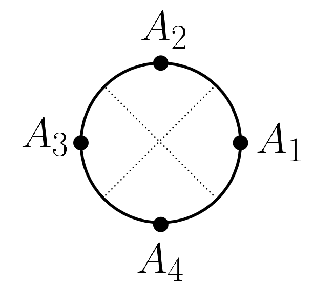
In the following, we use a pictorial representation of the correlation function on the unit disk in Figure 1.

Refer to caption — Figure 1: A pictorial representation of the correlation function on the disk (2.72). The insertions of the vertex operators $g_{1}\circ A_{1}(0)$ , $g_{2}\circ A_{2}(0)$ , $g_{3}\circ A_{3}(0)$ , and $g_{4}\circ A_{4}(0)$ are represented by dots on the boundary of the disk.

We define a Grassmann-even operator $\mathcal{L}_{t}^{\text{stub}}$ by

\langle\,A_{1},V_{2}^{\text{stub}}(V_{2}^{\text{stub}}(A_{2},A_{3}),A_{4})\,\rangle=\,\langle\,\mathcal{L}_{t}^{\text{stub}}g_{1}\circ A_{1}(0)\,g_{2}\circ A_{2}(0)\,g_{3}\circ A_{3}(0)\,g_{4}\circ A_{4}(0))\,\rangle_{D}

(2.74)

and $\mathcal{L}_{s}^{\text{stub}}$ by

\langle\,A_{1},V_{2}^{\text{stub}}(A_{2},V_{2}^{\text{stub}}(A_{3},A_{4}))\,\rangle=\,\langle\,\mathcal{L}_{s}^{\text{stub}}g_{1}\circ A_{1}(0)\,g_{2}\circ A_{2}(0)\,g_{3}\circ A_{3}(0)\,g_{4}\circ A_{4}(0))\,\rangle_{D}\,.

(2.75)

Let us calculate $\mathcal{L}_{t}^{\text{stub}}$ . We find

\langle\,A_{1},V_{2}^{\text{stub}}(V_{2}^{\text{stub}}(A_{2},A_{3}),A_{4})\,\rangle=\,\langle\,e^{-wL_{0}}A_{1},e^{-2wL_{0}}\,(e^{-wL_{0}}A_{2}\ast e^{-wL_{0}}A_{3})\,\ast e^{-wL_{0}}A_{4}\,\rangle\,.

(2.76)

We would like to express the right-hand side of this equation in terms of the correlation function on the disk $D$ . Therefore, we introduce the line integral $L_{0}[f]$ for a conformal transformation $f(\xi)$ by

L_{0}[f]=\oint\frac{dz}{2\pi i}\,f^{-1}(z)\left(\frac{df^{-1}(z)}{dz}\right)^{-1}\,T(z)\quad\text{with}\quad z=f(\xi)\,.

(2.77)

then we have

	$\displaystyle\langle\,e^{-wL_{0}}A_{1},A_{2}\ast A_{3}\ast A_{4}\,\rangle=$	$\displaystyle\ \langle\,e^{-wL_{0}[g_{1}]}\,g_{1}\circ A_{1}(0)\,g_{2}\circ A_{2}(0)\,g_{3}\circ A_{3}(0)\,g_{4}\circ A_{4}(0)\,\rangle_{D}\,,$
	$\displaystyle\langle\,A_{1},(e^{-wL_{0}}A_{2})\ast A_{3}\ast A_{4}\,\rangle=$	$\displaystyle\ \langle\,e^{-wL_{0}[g_{2}]}\,g_{1}\circ A_{1}(0)\,g_{2}\circ A_{2}(0)\,g_{3}\circ A_{3}(0)\,g_{4}\circ A_{4}(0)\,\rangle_{D}\,,$
	$\displaystyle\langle\,A_{1},A_{2}\ast(e^{-wL_{0}}A_{3})\ast A_{4}\,\rangle=$	$\displaystyle\ \langle\,e^{-wL_{0}[g_{3}]}\,g_{1}\circ A_{1}(0)\,g_{2}\circ A_{2}(0)\,g_{3}\circ A_{3}(0)\,g_{4}\circ A_{4}(0)\,\rangle_{D}\,,$
	$\displaystyle\langle\,A_{1},A_{2}\ast A_{3}\ast(e^{-wL_{0}}A_{4})\,\rangle=$	$\displaystyle\ \langle\,e^{-wL_{0}[g_{4}]}\,g_{1}\circ A_{1}(0)\,g_{2}\circ A_{2}(0)\,g_{3}\circ A_{3}(0)\,g_{4}\circ A_{4}(0)\,\rangle_{D}\,.$

Here and in what follows, we express a correlation function with insertions of these operators by a disk with solid lines. See Figure 2.

Furthermore, we use other functions $h_{1}(\xi)$ , $h_{2}(\xi)$ , $h_{3}(\xi)$ , and $h_{4}(\xi)$ on the disk $D$ defined by

\begin{split}&h_{1}(\xi)=e^{\pi i/4}\left(\frac{1+i\xi}{1-i\xi}\right)\,,\quad h_{2}(\xi)=e^{3\pi i/4}\left(\frac{1+i\xi}{1-i\xi}\right)\,,\\ &h_{3}(\xi)=e^{5\pi i/4}\left(\frac{1+i\xi}{1-i\xi}\right)\,,\quad h_{4}(\xi)=e^{7\pi i/4}\left(\frac{1+i\xi}{1-i\xi}\right)\,.\end{split}

(2.78)

Then we have

	$\displaystyle\langle\,e^{-wL_{0}}(A_{1}\ast A_{2}),A_{3}\ast A_{4}\,\rangle=$	$\displaystyle\ \langle\,e^{-wL_{0}[h_{1}]}\,g_{1}\circ A_{1}(0)\,g_{2}\circ A_{2}(0)\,g_{3}\circ A_{3}(0)\,g_{4}\circ A_{4}(0)\,\rangle_{D}\,,$
	$\displaystyle\langle\,A_{1},e^{-wL_{0}}(A_{2}\ast A_{3})\ast A_{4}\,\rangle=$	$\displaystyle\ \langle\,e^{-wL_{0}[h_{2}]}\,g_{1}\circ A_{1}(0)\,g_{2}\circ A_{2}(0)\,g_{3}\circ A_{3}(0)\,g_{4}\circ A_{4}(0)\,\rangle_{D}\,,$
	$\displaystyle\langle\,A_{1},A_{2}\ast e^{-wL_{0}}(A_{3}\ast A_{4})\,\rangle=$	$\displaystyle\ \langle\,e^{-wL_{0}[h_{3}]}\,g_{1}\circ A_{1}(0)\,g_{2}\circ A_{2}(0)\,g_{3}\circ A_{3}(0)\,g_{4}\circ A_{4}(0)\,\rangle_{D}\,,$
	$\displaystyle\langle\,A_{1},(e^{-wL_{0}})^{\star}(A_{2}\ast A_{3})\ast A_{4}\,\rangle=$	$\displaystyle\ \langle\,e^{-wL_{0}[h_{4}]}\,g_{1}\circ A_{1}(0)\,g_{2}\circ A_{2}(0)\,g_{3}\circ A_{3}(0)\,g_{4}\circ A_{4}(0)\,\rangle_{D}\,.$

These correlation functions are pictorially represented in Figure 3.

Using the definition of the two-string product $V_{2}^{\text{stub}}$ (2.65), we find

\mathcal{L}_{t}^{\text{stub}}=\ e^{-wL_{0}[g_{1}]}\,e^{-2wL_{0}[h_{2}]}\,e^{-wL_{0}[g_{2}]}\,e^{-wL_{0}[g_{3}]}\,e^{-wL_{0}[g_{4}]}\,.

(2.79)

By a similar calculation, we find

\mathcal{L}_{s}^{\text{stub}}=\ e^{-wL_{0}[g_{1}]}\,e^{-wL_{0}[g_{2}]}\,e^{-2wL_{0}[h_{3}]}\,e^{-wL_{0}[g_{3}]}\,e^{-wL_{0}[g_{4}]}\,.

(2.80)

Pictorial representations of $\mathcal{L}_{t}^{\text{stub}}$ and $\mathcal{L}_{s}^{\text{stub}}$ are given in Figure 4.

We define the three-string product $V_{3}^{\text{stub}}$ in terms of a Grassmann-odd operator $\mathcal{B}_{3}^{\text{stub}}$ :

\langle\,A_{1},V_{3}^{\text{stub}}(A_{2},A_{3},A_{4})\,\rangle=\,\langle\,g_{1}\circ A_{1}(0)\,\mathcal{B}_{3}^{\text{stub}}\,g_{2}\circ A_{2}(0)\,g_{3}\circ A_{3}(0)\,g_{4}\circ A_{4}(0)\,\rangle_{D}\,.

(2.81)

Then the $A_{\infty}$ relation for the three-string product $V_{3}^{\text{stub}}$

\begin{split}0=&\ QV_{3}^{\text{stub}}(A_{1},A_{2},A_{3})+V_{3}^{\text{stub}}(QA_{1},A_{2},A_{3})\\ &\quad+(-1)^{A_{1}}V_{3}^{\text{stub}}(A_{1},QA_{2},A_{3})+(-1)^{A_{1}+A_{2}}V_{3}^{\text{stub}}(A_{1},A_{2},QA_{3})\\ &\quad{}-V_{2}^{\text{stub}}(V_{2}^{\text{stub}}(A_{1},A_{2}),A_{3})+V_{2}^{\text{stub}}(A_{1},V_{2}^{\text{stub}}(A_{2},A_{3}))\end{split}

(2.82)

is translated into the following equation:

Q\cdot\mathcal{B}_{3}^{\text{stub}}=\ \mathcal{L}_{t}^{\text{stub}}-\mathcal{L}_{s}^{\text{stub}}\,.

(2.83)

To construct $\mathcal{B}_{3}^{\text{stub}}$ , it is convenient to use the extended BRST formalism [15]. The different factors between $\mathcal{L}_{t}$ and $\mathcal{L}_{s}$ are $e^{-2wL_{0}[h_{2}]}$ and $e^{-2wL_{0}[h_{3}]}$ , so we focus on these factors. Following the construction (2.58) in subsection 2.2, a naive solution is

\mathcal{B}^{\text{naive}}=\,\int_{0}^{1}dt\int d\tilde{t}\,e^{\{\,Q^{\prime}\,,\,\mathcal{F}^{\text{naive}}(t)\,\}}\,

(2.84)

with

\mathcal{F}^{\text{naive}}(t)=\,{}-2wtb_{0}[h_{2}]-2w(1-t)b_{0}[h_{3}]\,,

(2.85)

where we defined the line integral $b_{0}[f]$ for a conformal transformation $f(\xi)$ by

b_{0}[f]=\,\oint\frac{dz}{2\pi i}\,f^{-1}(z)\,\Bigl(\frac{df^{-1}(z)}{dz}\Bigr)^{-1}b(z)\quad\text{with}\quad z=f(\xi)\,.

(2.86)

Using

	$\displaystyle\{\,Q^{\prime}\,,\,\mathcal{F}^{\text{naive}}(t=1)\,\}=$	$\displaystyle\ \{\,Q\,,-2wb_{0}[h_{2}]\,\}={}-2wL_{0}[h_{2}]\,,$		(2.87)
	$\displaystyle\{\,Q^{\prime}\,,\,\mathcal{F}^{\text{naive}}(t=0)\,\}=$	$\displaystyle\ \{\,Q\,,-2wb_{0}[h_{3}]\,\}={}-2wL_{0}[h_{3}]\,,$		(2.88)

we can show that this operator interpolates between $e^{-2wL_{0}[h_{2}]}$ and $e^{-2wL_{0}[h_{3}]}$ :

Q\cdot\mathcal{B}^{\text{naive}}=\,e^{-2wL_{0}[h_{2}]}-e^{-2wL_{0}[h_{3}]}\,.

(2.89)

Instead of the operator $\mathcal{B}^{\text{naive}}$ , we introduce the operator $\mathcal{B}[f]$ in the following form:

\mathcal{B}[f]=\ \int_{0}^{1}dt\int d\tilde{t}\,e^{\{Q^{\prime},t(-2w)b_{0}[f]\}}\,.

(2.90)

The operator $\mathcal{B}[f]$ interpolates between the stub operator $e^{-2wL_{0}[f]}$ and the unit operator $1$ . Let us carry out the integration over $\tilde{t}$ . Since

\displaystyle\{\,Q^{\prime}\,,t(-2w)b_{0}[f]\,\}=

\displaystyle\ \tilde{t}(-2w)b_{0}[f]+t(-2w)L_{0}[f]\,,

(2.91)

we find

\displaystyle\mathcal{B}[f]=

\displaystyle\,{}-\int_{0}^{1}dt\,(-2w)b_{0}[f]e^{t(-2w)L_{0}[f]}\,.

(2.92)

The BRST transformation of $\mathcal{B}[f]$ is then

\begin{split}\,Q\cdot\mathcal{B}[f]=&\,-\int_{0}^{1}dt\,(-2w)L_{0}[f]e^{t(-2w)L_{0}[f]}\\ =&\,-\int_{0}^{1}dt\,\partial_{t}e^{t(-2w)L_{0}[f]}\\ =&\ 1-e^{-2wL_{0}[f]}\,.\end{split}

(2.93)

Since the operator $\mathcal{B}[f]$ interpolates the unit operator $1$ and the stub operator $e^{-2wL_{0}[f]}$ , we regard $\mathcal{B}[f]$ as an operator which creates the stub operator $e^{-2wL_{0}}$ , and we call this the stub creation operator. On the other hand, the operator $-\mathcal{B}[f]$ interpolates the unit operator and the stub operator in the reverse direction:

\,Q\cdot(-\mathcal{B}[f])=\,e^{-2wL_{0}[f]}-1\,.

(2.94)

Therefore, we call $-\mathcal{B}[f]$ the stub annihilation operator. Using the stub creation and annihilation operators, we find that $\mathcal{B}_{3}^{\text{stub}}$ is given by

\mathcal{B}_{3}^{\text{stub}}=(-\mathcal{B}[h_{2}]+\mathcal{B}[h_{3}])\,e^{-wL_{0}[g_{1}]}e^{-wL_{0}[g_{2}]}e^{-wL_{0}[g_{3}]}e^{-wL_{0}[g_{4}]}\,.

(2.95)

The interpolation by $\mathcal{B}_{3}^{\text{stub}}$ is illustrated in Figure 5.

Then the action of the BRST operator on $\mathcal{B}_{3}$ is given by

\begin{split}Q\cdot\mathcal{B}_{3}^{\text{stub}}=&\ \Bigl((e^{-2wL_{0}[h_{2}]}-1)+(1-e^{-2wL_{0}[f]})\Bigr)e^{-wL_{0}[g_{1}]}e^{-wL_{0}[g_{2}]}e^{-wL_{0}[g_{3}]}e^{-wL_{0}[g_{4}]}\\ =&\ \mathcal{L}_{t}^{\text{stub}}-\mathcal{L}_{s}^{\text{stub}}\,.\end{split}

(2.96)

Therefore, the three-string product $V_{3}^{\text{stub}}$ constructed from $\mathcal{B}_{3}^{\text{stub}}$ (2.95) satisfies the $A_{\infty}$ relation (2.82). In appendix B, we show that the three-string product $V_{3}^{\text{stub}}$ also satisfies the cyclicity equation

\langle\,A_{1},V_{3}^{\text{stub}}(A_{2},A_{3},A_{4})\,\rangle={}-(-1)^{A_{1}}\langle\,V_{3}^{\text{stub}}(A_{1},A_{2},A_{3}),A_{4}\,\rangle\,.

(2.97)

Therefore, the action constructed from the two-string product $V_{2}^{\text{stub}}$ (2.65) and the three-string product $V_{3}^{\text{stub}}$ (2.81) has the cyclic $A_{\infty}$ structure up to quartic order.

In the construction of open bosonic string field theory, the form of the $b$ ghost insertion in (2.92) is not complicated, and we may be able to construct it without using the extended BRST formalism. The extended BRST formalism plays a crucial role in the extension to the superstring.

3 The Neveu-Schwarz sector of open superstring field theory

In this section, we review the Neveu-Schwarz sector of open superstring field theory. Starting with an explanation of the extended BRST formalism for the superstring, we review the construction of an action for the Neveu-Schwarz sector of open superstring field theory based on the supermoduli space presented by Ohmori and Okawa [14].

3.1 Extended BRST formalism

Let us consider tree-level scattering amplitudes in the Neveu-Schwarz sector of the open superstring. If we use the superspace, the location of a vertex operator on the boundary is described by one Grassmann-even coordinate and one Grassmann-odd coordinate. Using global super-conformal transformations on the disk, we can fix three even coordinates and two odd coordinates. Therefore, disks with $n$ Neveu-Schwarz punctures on the boundary have $n-3$ even moduli and $n-2$ odd moduli. The integration over a Grassmann-odd modulus yields the local picture-changing operator. In the construction of superstring field theory, it is useful to consider other parametrizations of the supermoduli space of super-Riemann surfaces. Disks with three Neveu-Schwarz punctures have one odd modulus, and we denote it by $\zeta$ . We consider a parametrization of the supermoduli space of super-Riemann surfaces in the following form:

\int d\zeta e^{\zeta G_{-1/2}}\quad\text{with}\quad G_{-1/2}=\,\oint\frac{dz}{2\pi i}\,T_{\text{F}}(z)\,,

(3.1)

where $T_{F}(z)$ is the supercurrent. The integration over the odd modulus requires an associated ghost insertion. Following [15], we introduce a Grassmann-even variable $\tilde{\zeta}$ , and define an action of an extended BRST operator $Q^{\prime}$ by

\{\,Q^{\prime},\zeta\,\}=\,\tilde{\zeta}\,,\quad[\,Q^{\prime},\tilde{\zeta}\,]=\,0\,.

(3.2)

We can show that the extended BRST operator is nilpotent:

Q^{\prime 2}=0\,,

(3.3)

and we can express $Q^{\prime}$ as

Q^{\prime}=\,Q+\tilde{\zeta}\partial_{\zeta}\,.

(3.4)

The actions of the extended BRST operator on the states of the CFT are the same as those of the BRST operator $Q$ . In particular, we have

[\,Q^{\prime},\beta_{-1/2}\,]=G_{-1/2}\,,\quad\{\,Q^{\prime},G_{-1/2}\,\}=0\,,

(3.5)

where $\beta_{-1/2}$ is given by

\beta_{-1/2}=\,\oint\frac{dz}{2\pi i}\beta(z)\,.

(3.6)

Note that the combination $-\tilde{\zeta}\beta_{-1/2}+\zeta G_{-1/2}$ anti-commutes with $Q^{\prime}$ :

\{\,Q^{\prime}\,,-\tilde{\zeta}\beta_{-1/2}+\zeta G_{-1/2}\,\}=\,{}-\tilde{\zeta}G_{-1/2}+\tilde{\zeta}G_{-1/2}=\,0\,.

(3.7)

In fact, this combination can be generated by the action of $Q^{\prime}$ on $-\zeta\beta_{-1/2}$ :

-\tilde{\zeta}\beta_{-1/2}+\zeta G_{-1/2}=\,\{\,Q^{\prime}\,,-\zeta\beta_{-1/2}\,\}\,.

(3.8)

The integration over the odd modulus $\zeta$ can be combined with the associated ghost insertion to yield the picture-changing operator⁴⁴ 4 The subscript N denotes that this is the picture-changing operator which acts on Neveu-Schwarz string fields. In the next section, we will introduce the picture-changing operator $X_{\text{R}}$ which acts on Ramond string fields.

X_{\text{N}}=\,\int d\zeta d\tilde{\zeta}\mathcal{X}_{\text{N}}(\zeta,\tilde{\zeta})\,,

(3.9)

where

\mathcal{X}_{\text{N}}(\zeta,\tilde{\zeta})=\ e^{-\{Q^{\prime},\,\zeta\beta_{-1/2}\,\}}=\ e^{-\tilde{\zeta}\beta_{-1/2}+\zeta G_{-1/2}}\,.

(3.10)

By using the Baker-Hausdorff-Campbell formula and carrying out an integration over $\zeta$ , the explicit expression of the operator $X_{\text{N}}$ is given by

\displaystyle X_{\text{N}}=G_{-1/2}\,\delta(\beta_{-1/2})+b_{-1}\,\delta^{\prime}(\beta_{-1/2})\,,

(3.11)

where the delta function operators are defined by

\displaystyle\delta(\beta_{-1/2})=\,\int d\tilde{\zeta}e^{-\tilde{\zeta}\beta_{-1/2}}\,,\quad\delta^{\prime}(\beta_{-1/2})={}-\int d\tilde{\zeta}\,\tilde{\zeta}\,e^{-\tilde{\zeta}\beta_{-1/2}}\,.

(3.12)

It is emphasized in [15] that the integration over a Grassmann-even variable $\tilde{\zeta}$ should be understood as an algebraic operation, and we give its definition in appendix A. We treat the measure $d\tilde{\zeta}$ as a Grassmann-odd object for the reason we will explain in appendix A, therefore the delta functions $\delta(\beta_{-1/2})$ and $\delta^{\prime}(\beta_{-1/2})$ are Grassmann-odd. The picture-changing operator $X_{\text{N}}$ carries the picture number $1$ , and $X_{\text{N}}$ commutes with the BRST operator:

\begin{split}[\,Q,X_{\text{N}}\,]=&\ \int\int d\zeta d\tilde{\zeta}\,\{\,Q,\mathcal{X}_{\text{N}}(\zeta,\tilde{\zeta})\,\}\\ =&\ -\int\int d\zeta d\tilde{\zeta}\tilde{\zeta}\partial_{\zeta}\mathcal{X}_{\text{N}}(\zeta,\tilde{\zeta})\\ =&\ 0\,,\end{split}

(3.13)

where we replaced $Q$ acting on $\mathcal{X}_{\text{N}}(\zeta,\tilde{\zeta})$ by $-\tilde{\zeta}\partial_{\zeta}$ since $\mathcal{X}_{\text{N}}(\zeta,\tilde{\zeta})$ anti-commutes with $Q^{\prime}$ .

3.2 Kinetic term for the Neveu-Schwarz sector

Let us consider the Neveu-Schwarz sector of open superstring field theory. The Neveu-Schwarz string field $\Psi_{\text{N}}$ is a state in the Hilbert space of the boundary CFT describing the open superstring background we consider, which consists of the matter sector, the $bc$ ghost sector, and the $\beta\gamma$ ghost sector. We choose the Neveu-Schwarz string field $\Psi$ to be a Grassmann-odd state of ghost number $1$ and picture number $-1$ . The BPZ inner product for the superstring has the same properties as the BPZ inner product of bosonic string field theory, except that the BPZ inner product for the superstring is well defined only when the sum of the picture numbers of inputs is equal to $-2$ . The kinetic term of the Neveu-Schwarz string field is

{}-\frac{1}{2}\langle\,\Psi_{\text{N}},Q\Psi_{\text{N}}\,\rangle\,,

(3.14)

where $Q$ is the BRST operator of the world-sheet theory of the superstring. This kinetic term is invariant under the gauge transformation:

\delta\Psi_{\text{N}}=Q\Lambda_{\text{N}}\,,

(3.15)

where $\Lambda_{\text{N}}$ is a Grassmann-even state of ghost number $0$ in the $-1$ picture.

3.3 Cubic vertex for the Neveu-Schwarz sector

Let us consider a cubic vertex for the Neveu-Schwarz string fields. We construct a cubic vertex for the Neveu-Schwarz string fields in terms of the two-string product which satisfies the cyclicity equation

\langle\,N_{1},V_{2}(N_{2},N_{3})\,\rangle=\,\langle\,V_{2}(N_{1},N_{2}),N_{3}\,\rangle

(3.16)

and the $A_{\infty}$ relation

0=\ QV_{2}(N_{1},N_{2})-V_{2}(QN_{1},N_{2})-(-1)^{N_{1}}V_{2}(N_{1},QN_{2})\,,

(3.17)

where $N_{1}$ and $N_{2}$ are Neveu-Schwarz string fields in the $-1$ picture. As we have seen in subsection 3.1, disks with three Neveu-Schwarz punctures have one odd modulus, and we denote it by $\zeta$ . In the construction by Ohmori and Okawa in [14], an integral over the odd modulus is implemented by an insertion of the picture-changing operator $X_{\text{N}}$ (3.9). Then we consider the cubic vertex for the Neveu-Schwarz string fields of the form

S_{\text{N}}=\,\langle\,X_{\text{N}}\Psi_{\text{N}},\Psi_{\text{N}}\ast\Psi_{\text{N}}\,\rangle\,.

(3.18)

By varying the cubic vertex $S_{\text{N}}$ with respect to the Neveu-Schwarz string field $\Psi_{\text{N}}$ , we find

\delta S_{\text{N}}=\,\langle\,\delta\Psi,{X_{\text{N}}}^{\star}(\Psi_{\text{N}}\ast\Psi_{\text{N}})+X_{\text{N}}\Psi_{\text{N}}\ast\Psi_{\text{N}}+\Psi_{\text{N}}\ast X_{\text{N}}\Psi_{\text{N}}\,\rangle\,,

(3.19)

where $\mathcal{O}^{\star}$ represents the BPZ conjugate of an operator $\mathcal{O}$ . In the construction of an action by Ohmori and Okawa in [14], the two-string product $V_{2}$ in the following form is introduced:

V_{2}(N_{1},N_{2})=\ \frac{1}{3}\Bigl({X_{\text{N}}}^{\star}(N_{1}\ast N_{2})+X_{\text{N}}N_{1}\ast N_{2}+N_{1}\ast X_{\text{N}}N_{2}\Bigr)\,.

(3.20)

We can show that this two-string product (3.20) satisfies the cyclicity equation. We find

\begin{split}\ \langle\,N_{1},V_{2}(N_{2},N_{3})\,\rangle=&\ \frac{1}{3}(\,\langle\,N_{1},X_{\text{N}}^{\star}(N_{2}\ast N_{3})\,\rangle+\langle\,N_{1},X_{\text{N}}N_{2}\ast N_{3}\,\rangle+\langle\,N_{1},N_{2}\ast X_{\text{N}}N_{3}\,\rangle\,)\\ =&\ \frac{1}{3}(\,\langle\,X_{\text{N}}N_{1},N_{2}\ast N_{3}\,\rangle+\langle\,N_{1}\ast X_{\text{N}}N_{2},N_{3}\,\rangle+\langle\,N_{1}\ast N_{2},X_{\text{N}}N_{3}\,\rangle)\\ =&\ \frac{1}{3}(\,\langle\,X_{\text{N}}N_{1}\ast N_{2},N_{3}\,\rangle+\langle\,N_{1},X_{\text{N}}N_{2}\ast N_{3}\,\rangle+\langle\,X_{\text{N}}^{\star}(N_{1}\ast N_{2}),N_{3}\,\rangle\,)\\ =&\ \langle\,N_{1},V_{2}(N_{2},N_{3})\,\rangle\,,\end{split}

(3.21)

where we used the equation (2.8). We can show that this product satisfies the $A_{\infty}$ relation. We find

\begin{split}QV_{2}(N_{1},N_{2})=&\ \frac{1}{3}(\,QX_{\text{N}}^{\star}(N_{1}\ast N_{2})+Q(X_{\text{N}}N_{1}\ast N_{2})+Q(N_{1}\ast X_{\text{N}}N_{2})\,)\\ =&\ \frac{1}{3}(\,X_{\text{N}}^{\star}Q(N_{1}\ast N_{2})+QX_{\text{N}}N_{1}\ast N_{2}+(-1)^{N_{1}}X_{\text{N}}N_{1}\ast QN_{2}\\ &\quad+QN_{1}\ast X_{\text{N}}N_{2}+(-1)^{N_{1}}N_{1}\ast QX_{\text{N}}N_{2}\,)\\ =&\ \frac{1}{3}(\,X_{\text{N}}^{\star}(QN_{1}\ast N_{2})+(-1)^{N_{1}}X^{\star}(N_{1}\ast QN_{2})+X_{\text{N}}QN_{1}\ast N_{2}\\ &\quad+(-1)^{N_{1}}X_{\text{N}}N_{1}\ast QN_{2}+QN_{1}\ast X_{\text{N}}N_{2}+(-1)^{N_{1}}N_{1}\ast X_{\text{N}}QN_{2}\,)\\ =&\ V_{2}(QN_{1},N_{2})+(-1)^{N_{1}}V_{2}(N_{1},QN_{2})\,,\end{split}

(3.22)

where we used the equations (2.3) and (3.13).

Let us see that the two-string product (3.20) is not associative. We find

\begin{split}&V_{2}(V_{2}(N_{1},N_{2}),N_{3})\\ =&\ \frac{1}{9}\Bigl(\,X_{\text{N}}^{\star}X_{\text{N}}^{\star}(N_{1}\ast N_{2})\ast N_{3}+X_{\text{N}}X_{\text{N}}^{\star}(N_{1}\ast N_{2})\ast N_{3}+X_{\text{N}}^{\star}(N_{1}\ast N_{2})\ast X_{\text{N}}N_{3}\\ &\quad+X_{\text{N}}^{\star}(X_{\text{N}}N_{1}\ast N_{2}\ast N_{3})+X_{\text{N}}(X_{\text{N}}N_{1}\ast N_{2})\ast N_{3}+X_{\text{N}}N_{1}\ast N_{2}\ast X_{\text{N}}N_{3}\\ &\quad+X_{\text{N}}^{\star}(N_{1}\ast X_{\text{N}}N_{2}\ast N_{3})+X_{\text{N}}(N_{1}\ast X_{\text{N}}N_{2})\ast N_{3}+N_{1}\ast X_{\text{N}}N_{2}\ast X_{\text{N}}N_{3}\,\Bigr)\\ \end{split}

(3.23)

and

\begin{split}&V_{2}(N_{1},V_{2}(N_{2},N_{3}))\\ =&\ \frac{1}{9}\Bigl(\,X_{\text{N}}^{\star}N_{1}\ast X_{\text{N}}^{\star}(N_{2}\ast N_{3})+X_{\text{N}}N_{1}\ast X_{\text{N}}^{\star}(N_{2}\ast N_{3})+N_{1}\ast X_{\text{N}}X_{\text{N}}^{\star}(N_{2}\ast N_{3})\\ &\quad+X_{\text{N}}^{\star}(N_{1}\ast X_{\text{N}}N_{2}\ast N_{3})+X_{\text{N}}N_{1}\ast X_{\text{N}}N_{2}\ast N_{3}+N_{1}\ast X_{\text{N}}(X_{\text{N}}N_{2}\ast N_{3})\\ &\quad+X_{\text{N}}^{\star}(N_{1}\ast N_{2}\ast X_{\text{N}}N_{3})+X_{\text{N}}N_{1}\ast N_{2}\ast X_{\text{N}}N_{3}+N_{1}\ast X_{\text{N}}(N_{2}\ast X_{\text{N}}N_{3})\,\Bigr)\,.\\ \end{split}

(3.24)

Since the picture-changing operators are inserted in a different manner in (3.23) and (3.24), the two-string product (3.20) is not associative:

V_{2}(V_{2}(N_{1},N_{2}),N_{3})\neq V_{2}(N_{1},V_{2}(N_{2},N_{3}))\,.

(3.25)

We can recover the gauge-invariance at quartic order by constructing a three-string product $V_{3}(N_{1},N_{2},N_{3})$ satisfying the $A_{\infty}$ relation (2.21).

3.4 Quartic vertex for the Neveu-Schwarz sector

Let us consider a quartic vertex for the Neveu-Schwarz sector. We express a quartic vertex in terms of a three-string product $V_{3}(N_{1},N_{2},N_{3})$ . As we demonstrated in the case of open bosonic string field theory with stubs, we construct three-string product by interpolating the $t$ -channel contribution and the $s$ -channel contribution.

We introduce the line integral $X_{\text{N}}[f]$ by

\displaystyle X_{\text{N}}[f]=\int d\zeta d\tilde{\zeta}e^{-\{Q^{\prime},\zeta\beta_{-1/2}[f]\}}\quad\text{with}\quad z=f(\xi)\,,

(3.26)

where $\beta_{-1/2}[f]$ is the line integral mapped from $\beta_{-1/2}$ by the conformal transformation $f(\xi)$ :

\displaystyle\beta_{-1/2}[f]=\oint\frac{dz}{2\pi i}\Bigl(\frac{df^{-1}(z)}{dz}\Bigr)^{-1/2}\beta(z)\quad\text{with}\quad z=f(\xi)\,.

(3.27)

Using the line integral $X_{\text{N}}$ , we can express the picture-changing operator in the BPZ inner product by an operator insertion on the correlation function. For example, we find

	$\displaystyle\ \langle\,N_{1},X_{\text{N}}N_{2}\ast N_{3}\ast N_{4})\,\rangle=$	$\displaystyle\ \langle\,X_{\text{N}}[g_{2}]\,g_{1}\circ N_{1}(0)\,g_{2}\circ N_{2}(0)\,g_{3}\circ N_{3}(0)\,g_{4}\circ N_{4}(0)\,\rangle_{D}\,,$		(3.28)
	$\displaystyle\ \langle\,N_{1},N_{2}\ast X_{\text{N}}(N_{3}\ast N_{4}))\,\rangle=$	$\displaystyle\ \langle\,X_{\text{N}}[h_{3}]\,g_{1}\circ N_{1}(0)\,g_{2}\circ N_{2}(0)\,g_{3}\circ N_{3}(0)\,g_{4}\circ N_{4}(0)\,\rangle_{D}\,.$		(3.29)

We define a Grassmann-even operator $X_{t}$ by

\ \langle\,N_{1},V_{2}(V_{2}(N_{2},N_{3}),N_{4})\,\rangle=\,\langle\,X_{t}\,g_{1}\circ N_{1}(0)\,g_{2}\circ N_{2}(0)\,g_{3}\circ N_{3}(0)\,g_{4}\circ N_{4}(0)\,\rangle_{D}\,,\\

(3.30)

and we can calculate $X_{t}$ from the definition of $V_{2}(N_{1},N_{2})$ (3.20). We find that

\displaystyle X_{t}=

\displaystyle\ \frac{1}{9}\Bigl(\,X_{\text{N}}[h_{4}]+X_{\text{N}}[g_{2}]+X_{\text{N}}[g_{3}]\,\Bigr)\Bigl(\,X_{\text{N}}[g_{1}]+X_{\text{N}}[h_{2}]+X_{\text{N}}[g_{4}]\,\Bigr)\,.

(3.31)

We define a Grassmann-even operator $X_{s}$ by

\ \langle\,N_{1},V_{2}(N_{2},V_{2}(N_{3},N_{4}))\,\rangle=\,\langle\,X_{s}\,g_{1}\circ N_{1}(0)\,g_{2}\circ N_{2}(0)\,g_{3}\circ N_{3}(0)\,g_{4}\circ N_{4}(0)\,\rangle_{D}\,,

(3.32)

and we find

\displaystyle X_{s}=

\displaystyle\ \frac{1}{9}\Bigl(\,X_{\text{N}}[h_{1}]+X_{\text{N}}[g_{3}]+X_{\text{N}}[g_{4}]\,\Bigr)\Bigl(\,X_{\text{N}}[g_{2}]+X_{\text{N}}[h_{3}]+X_{\text{N}}[g_{1}]\,\Bigr)\,.

(3.33)

We express the three-string product $V_{3}(N_{1},N_{2},N_{3})$ in terms of a Grassmann-odd operator $\Xi$ :

\ \langle\,N_{1},V_{3}(N_{2},N_{3},N_{4})\,\rangle=\,\langle\,g_{1}\circ N_{1}(0)\,\Xi\,g_{2}\circ N_{2}(0)\,g_{3}\circ N_{3}(0)\,g_{4}\circ N_{4}(0)\,\rangle_{D}\,.

(3.34)

Then the $A_{\infty}$ relation

\begin{split}0=&\ QV_{3}(N_{1},N_{2},N_{3})+V_{3}(QN_{1},N_{2},N_{3})\\ &\quad+(-1)^{N_{1}}V_{3}(N_{1},QN_{2},N_{3})+(-1)^{N_{1}+N_{2}}V_{3}(N_{1},N_{2},QN_{3})\\ &\quad{}-V_{2}(V_{2}(N_{1},N_{2}),N_{3})+V_{2}(N_{1},V_{2}(N_{2},N_{3}))\end{split}

(3.35)

is translated into the following equation:

\displaystyle Q\cdot\Xi=

\displaystyle\ X_{t}-X_{s}\,.

(3.36)

In [14], the following operator is introduced as building blocks for the construction of $\Xi$ :

\Xi[a,b]=\int_{0}^{1}dt\int d\tilde{t}\int d\zeta d\tilde{\zeta}\ e^{-\{Q^{\prime},t\zeta\beta_{-1/2}[a]\}}\ e^{-\{Q^{\prime},(1-t)\zeta\beta_{-1/2}[b]\}}\,,

(3.37)

where

Q^{\prime}=\,Q+\tilde{\zeta}\partial_{\zeta}+\tilde{t}\partial_{t}\,,

(3.38)

and $a$ , $b$ are some integration contours $g_{i}$ , $h_{i}$ $(i=1,2,3,4)$ on the disk $D$ . This operator interpolates between the picture-chainging operators $X_{\text{N}}[a]$ and $X_{\text{N}}[b]$ :

Q\cdot\Xi[a,b]=X_{\text{N}}[a]-X_{\text{N}}[b]\,,

(3.39)

and it is anti-symmetric about the integration contours $a$ and $b$ :

\Xi[a,b]=-\Xi[b,a]\,,

(3.40)

The equation (3.39) can be shown in the following way:

\begin{split}\,Q\cdot\Xi[a,b]=&\,\int_{0}^{1}dt\int d\tilde{t}\int d\zeta d\tilde{\zeta}\ Q\cdot\left(\,e^{-\{Q^{\prime},t\zeta\beta_{-1/2}[a]\}}\ e^{-\{Q^{\prime},(1-t)\zeta\beta_{-1/2}[b]\}}\,\right)\\ =&\,{}-\int_{0}^{1}dt\int d\tilde{t}\int d\zeta d\tilde{\zeta}\ \tilde{t}\partial_{t}\left(\,e^{-\{Q^{\prime},t\zeta\beta_{-1/2}[a]\}}\ e^{-\{Q^{\prime},(1-t)\zeta\beta_{-1/2}[b]\}}\,\right)\\ &\,{}-\int_{0}^{1}dt\int d\tilde{t}\int d\zeta d\tilde{\zeta}\ \tilde{\zeta}\partial_{\zeta}\left(\,e^{-\{Q^{\prime},t\zeta\beta_{-1/2}[a]\}}\ e^{-\{Q^{\prime},(1-t)\zeta\beta_{-1/2}[b]\}}\,\right)\,,\end{split}

(3.41)

where we replaced the action of $Q$ on $e^{-\{Q^{\prime},t\zeta\beta_{-1/2}[a]\}}\ e^{-\{Q^{\prime},(1-t)\zeta\beta_{-1/2}[b]\}}$ by that of $-\tilde{t}\partial_{t}-\tilde{\zeta}\partial_{\zeta}$ . The second term on the right-hand side of this equation vanishes, since it is an integration over total derivative of the Grassmann-odd variable. Then we find

\begin{split}\,Q\cdot\Xi[a,b]=&\,\int d\zeta d\tilde{\zeta}\,e^{-\{Q^{\prime},t\zeta\beta_{-1/2}[a]\}}\ e^{-\{Q^{\prime},(1-t)\zeta\beta_{-1/2}[b]\}}\,\Bigr|_{\tilde{t}=0}\\ &\quad\,{}-\int d\zeta d\tilde{\zeta}\,e^{-\{Q^{\prime},t\zeta\beta_{-1/2}[a]\}}\ e^{-\{Q^{\prime},(1-t)\zeta\beta_{-1/2}[b]\}}\,\Bigr|_{\tilde{t}=0}\\ =&\,\int d\zeta d\tilde{\zeta}\ e^{-\{Q^{\prime\prime},\zeta\beta_{-1/2}[a]\}}\,{}-\int d\zeta d\tilde{\zeta}\ e^{-\{Q^{\prime\prime},\zeta\beta_{-1/2}[b]\}}\,,\end{split}

(3.42)

where

Q^{\prime\prime}=Q+\tilde{\zeta}\partial_{\zeta}\,.

(3.43)

Therefore, the equation (3.39) is confirmed. To look at the operator $\Xi[a,b]$ in detail, let us expand $\Xi[a,b]$ and carry out the integral over $\tilde{t}$ and $\zeta$ . Since we have

	$\displaystyle\{\,Q^{\prime},t\zeta\beta_{-1/2}[a]\,\}=$	$\displaystyle\ {}-\tilde{t}\zeta\beta_{-1/2}-t\tilde{\zeta}\beta_{-1/2}-t\zeta G_{-1/2}\,,$		(3.44)
	$\displaystyle\{\,Q^{\prime},(1-t)\zeta\beta_{-1/2}[a]\,\}=$	$\displaystyle\ \tilde{t}\zeta\beta_{-1/2}-(1-t)\tilde{\zeta}\beta_{-1/2}-(1-t)\zeta G_{-1/2}\,,$		(3.45)

we find

\Xi[a,b]=\,\int_{0}^{1}dt\,(\beta_{-1/2}[a]-\beta_{-1/2}[b])\,\delta(t\beta_{-1/2}[a]+(1-t)\beta_{-1/2}[b])\,.

(3.46)

Correlation functions which contain the operator $\delta(t\beta_{-1/2}[a]+(1-t)\beta_{-1/2}[b])$ look unfamiliar. An example of such correlation functions were explicitly calculated in [14], and it was found that the correlation function develops a double pole at $t=1/2$ . In general, when the gauge fixing of the world-sheet supergravity fails, the superconformal ghost sector develops a pole and such a pole is called a spurious pole. In the case of [14], the double pole can be avoided by deforming the contour, and the resulting integral does not depend on the defomation of the contour, since the correlation function does not develop a single pole. Therefore, correlation functions which contain the operator $\delta(t\beta_{-1/2}[a]+(1-t)\beta_{-1/2}[b])$ are unambiguously defined.

In [14], an operator $\Xi$ satisfying (3.36) is constructed. The final result is given by

\begin{split}\Xi=\ \frac{1}{18}\Bigl(&\ \Xi[h_{2},h_{4};h_{3},h_{1}]+\Xi[h_{2},g_{4};h_{3},g_{3}]+\Xi[h_{2},g_{3};h_{3},g_{4}]\\ &+\Xi[g_{4},h_{4};g_{1},h_{1}]+\Xi[g_{4},g_{2};g_{1},g_{3}]+\Xi[g_{4},g_{3};g_{1},g_{4}]\\ &+\Xi[g_{1},h_{4};g_{2},h_{1}]+\Xi[g_{1},g_{2};g_{2},g_{3}]+\Xi[g_{1},g_{3};g_{2},g_{4}]\\ &-\Xi[h_{3},h_{1};h_{4},h_{2}]-\Xi[h_{3},g_{3};h_{4},g_{4}]-\Xi[h_{3},g_{4};h_{4},g_{1}]\\ &-\Xi[g_{1},h_{1};g_{2},h_{2}]-\Xi[g_{1},g_{3};g_{2},g_{4}]-\Xi[g_{1},g_{4};g_{2},g_{1}]\\ &-\Xi[g_{2},h_{1};g_{3},h_{2}]-\Xi[g_{2},g_{3};g_{3},g_{4}]-\Xi[g_{2},g_{4};g_{3},g_{1}]\ \Bigr)\,,\end{split}

(3.47)

where

\begin{split}\Xi[a_{1},a_{2};b_{1},b_{2}]=\frac{1}{2}\Bigl(&\,\Xi[a_{1},b_{1}]X_{\text{N}}[a_{2}]+X_{\text{N}}[b_{1}]\Xi[a_{2},b_{2}]\\ &+X_{\text{N}}[a_{1}]\Xi[a_{2},b_{2}]+\Xi[a_{1},b_{1}]X_{\text{N}}[b_{2}]\,\Bigr)\,,\end{split}

(3.48)

and $a_{1}$ , $b_{1}$ , $a_{2}$ , $b_{2}$ are integration contours $g_{i},h_{i}\ (i=1,2,3,4)$ on the disk. The two-string product $V_{2}(N_{1},N_{2})$ (3.20) and the three-string product $V_{3}(N_{1},N_{2},N_{3})$ (3.34) constructed from the Grassmann-odd operator $\Xi$ satisfies the $A_{\infty}$ relation (3.35) and the cyclicity equation

\langle\,N_{1},V_{3}(N_{2},N_{3},N_{4})\,\rangle={}-(-1)^{N_{1}}\langle\,V_{3}(N_{1},N_{2},N_{3}),N_{4}\,\rangle\,.

(3.49)

Therefore, the action constructed from the two-string product $V_{2}(N_{1},N_{2})$ (3.20) and the three-string product $V_{3}(N_{1},N_{2},N_{3})$ (3.34) has the cyclic $A_{\infty}$ structure up to quartic order.

4 Open superstring field theory including the Ramond sector

In this section, we consider open superstring field theory including the Ramond sector. Following the paper [9], we review the kinetic term of the Ramond sector of open superstring field theory by comparison with closed bosonic string field theory. After describing the cubic vertex including the Ramond sector, we construct the quartic vertices including the Ramond sector in the same manner as the Neveu-Schwarz sector.

4.1 The kinetic term for the Ramond sector

Recentry, a complete action for open superstring field theory including the Ramond sector was constructed by Kunitomo and Okawa [9]. We explain an interpretation of the kinetic term for the Ramond sector in the context of the supermoduli space of super-Riemann surfaces by comparing it with closed bosonic string field theory.⁵⁵ 5 The content of this subsection is based on the paper by Kunitomo and Okawa [9].

The propagator strip in open bosonic string field theory [1] can be generated by the zero mode of Virasoro operator $L_{0}$ as $e^{-tL_{0}}$ , and the parameter $t$ is the modulus corresponding to the length of the strip. The integration over this modulus is implemented by the propagator in Siegel gauge as

\frac{b_{0}}{L_{0}}=\,\int_{0}^{\infty}dtb_{0}e^{-tL_{0}}\,,

(4.1)

where $b_{0}$ is the ghost insertion associated with the integration over the modulus $t$ .

The propagatpor surfece in closed bosonic string field theory [16] can be generated by the Virasoro generators $L_{0}+\tilde{L_{0}}$ and $i(L_{0}-\tilde{L_{0}})$ as $e^{-t(L_{0}+\tilde{L_{0}})+\theta i(L_{0}-\tilde{L_{0}})}$ , where $\tilde{L}_{0}$ is the zero mode of the anti-holomorphic part of the energy momentum tensor, and $t$ and $\theta$ are moduli. In closed string field theory, the integration over $t$ is implemented by the propagator

\frac{b_{0}^{+}}{L_{0}^{+}}=\,\int_{0}^{\infty}b_{0}^{+}e^{-tL_{0}^{+}}

(4.2)

in the Siegel gauge

b_{0}^{+}\Psi=\,0\,,

(4.3)

where

b_{0}^{+}=\,b_{0}+\tilde{b_{0}}\,,\quad L_{0}^{+}=L_{0}+\tilde{L_{0}}\,,

(4.4)

and $\tilde{b}_{0}$ is the zero mode of the anti-holomorphic part of the $b$ ghost. The ghost insertion associated with the integration over the modulus $t$ is $b_{0}^{+}$ . The integration over $\theta$ is implemented as a restriction on the Hilbert space of closed string fields. The integration over $\theta$ yields the operator of the form

B=\,b_{0}^{-}\,\int_{0}^{2\pi}\,\frac{d\theta}{2\pi}e^{i\theta L_{0}^{-}}\,,

(4.5)

where

b_{0}^{-}=\,b_{0}-\tilde{b_{0}}\,,\quad L_{0}^{-}=L_{0}-\tilde{L_{0}}\,,

(4.6)

and $b_{0}^{-}$ is the ghost insertion associated with integration over the modulus $\theta$ . The operator $B$ can be schematically understood as $\delta(b_{0}^{-})\,\delta(L_{0}^{-})$ . The closed bosonic string field $\Psi$ of ghost number $2$ is restricted to satisfy

b_{0}^{-}\Psi=\,0\,,\quad L_{0}^{-}\Psi=\,0\,.

(4.7)

It is known that the BRST cohomology on this restricted space gives the correct spectrum of the closed bosonic string. The appropriate inner product for restricted string fields $\Psi_{1}$ and $\Psi_{2}$ can be written as

\langle\,\Psi_{1},c_{0}^{-}\Psi_{2}\,\rangle\,,

(4.8)

where

c_{0}^{-}=\,\frac{1}{2}(c_{0}-\tilde{c}_{0})\,,

(4.9)

and $\tilde{c}_{0}$ is the zero mode of the anti-holomorphic part of the $c$ ghost. The kinetic term of the restricted string field is given by

S={}-\frac{1}{2}\langle\,\Psi,c_{0}^{-}Q\Psi\,\rangle\,,

(4.10)

where $Q$ is the BRST operator of the closed bosonic string. The operator $B$ can also be written as

B=\,-i\,\int_{0}^{2\pi}\,\frac{d\theta}{2\pi}\int d\tilde{\theta}e^{i\theta L_{0}^{-}+i\tilde{\theta}b_{0}^{-}}\,,

(4.11)

where $\tilde{\theta}$ is a Grassmann-odd variable. We can introduce the extended BRST operator $Q^{\prime}$ for closed superstring field theory, which maps $\theta$ to $\tilde{\theta}$ and $\tilde{\theta}$ to $0$ . Then the operator $B$ can be written in the following form:

B=\,-i\,\int_{0}^{2\pi}\,\frac{d\theta}{2\pi}\int d\tilde{\theta}e^{\{\,Q^{\prime}\,,\,i\theta b_{0}^{-}\,\}}\,.

(4.12)

The closed string field satisfying the restriction can be characterized as

Bc_{0}^{-}\Psi=\,\Psi\,.

(4.13)

Let us consider the kinetic term for the Ramond sector of open superstring field theory. The fermionic direction of the moduli space can be parameterized as $e^{\zeta G_{0}}$ , where $\zeta$ is the odd modulus. As is the case with the Neveu-Schwarz sector of the open superstring (3.9), the integration over $\zeta$ with an associated ghost insertion yields the operator $X_{\text{R}}$ ⁶⁶ 6 The subscript R denotes that this is the picture-changing operator for the Ramond sector.

X_{\text{R}}=\int d\zeta\int d\tilde{\zeta}e^{\zeta G_{0}-\tilde{\zeta}\beta_{0}}\,,

(4.14)

where $\tilde{\zeta}$ is a Grassmann-even variable, $\beta_{0}$ is the zero mode of the $\beta$ ghost, and $G_{0}$ is the zero mode of the supercurrent:

\beta_{0}=\ \oint\frac{dz}{2\pi i}z^{1/2}\,\beta(z)\,,\quad G_{0}=\oint\frac{dz}{2\pi i}z^{1/2}\,T_{\text{F}}(z)\,.

(4.15)

We note that $X_{\text{R}}$ is BPZ even:

X_{\text{R}}^{\star}=\ X_{\text{R}}\,.

(4.16)

The appropriate innter product of restrected string fields $R_{1}$ and $R_{2}$ in the $-1/2$ picture can be written as

\langle\,R_{1},Y_{\text{R}}R_{2}\,\rangle

(4.17)

with

Y_{\text{R}}=\,{}-c_{0}\delta^{\prime}(\gamma_{0})\,,

(4.18)

where $\delta^{\prime}(\gamma_{0})$ is defined by an integral over a Grassmann-even variable $\sigma$ :

\delta^{\prime}(\gamma_{0})=\int d\sigma\sigma e^{\sigma\gamma_{0}}\,.

(4.19)

As in the case of $\delta(\beta_{-1/2})$ and $\delta^{\prime}(\beta_{-1/2})$ , $\delta^{\prime}(\gamma_{0})$ is also a Grassmann-odd operator. We choose the Ramond string field $\Psi_{\text{R}}$ to be a Grassmann-odd state of ghost number $1$ and picture number $-1/2$ . It is known that the BRST cohomology on this restricted space gives the correct spectrum of the Ramond sector of open superstring [17, 18, 19]. In [20, 17, 19], the kinetic term for the restricted Ramond string field is given by

{}-\frac{1}{2}\langle\,\Psi_{\text{R}},Y_{\text{R}}Q\Psi_{\text{R}}\,\rangle\,.

(4.20)

The Ramond string field in the restricted space is characterized by the following equation [21]:

X_{\text{R}}Y_{\text{R}}\Psi_{\text{R}}=\,\Psi_{\text{R}}\,.

(4.21)

This is analogous to the characterization for the closed bosonic string field (4.13).

As is the case with the picture-changing operator for the Neveu-Schwarz sector, we can write $X_{\text{R}}$ using the extended BRST operator $Q^{\prime}$ :

X_{\text{R}}=\ \int d\zeta d\tilde{\zeta}\mathcal{X}_{\text{R}}(\zeta,\tilde{\zeta})\,,\quad\mathcal{X}_{\text{R}}(\zeta,\tilde{\zeta})=\ e^{\{Q^{\prime},-\zeta\beta_{0}\}}\,.

(4.22)

Then we can show that

[\,Q,X_{\text{R}}\,]=0\,.

(4.23)

The explicit form of $X_{\text{R}}$ is given by

X_{\text{R}}=\,G_{0}\delta(\beta_{0})+b_{0}\delta^{\prime}(\gamma_{0})\,,

(4.24)

where $\delta(\beta_{0})$ and $\delta^{\prime}(\beta_{0})$ are defined by

	$\displaystyle\delta(\beta_{0})=$	$\displaystyle\,\int d\tilde{\zeta}e^{-\tilde{\zeta}\beta_{0}}\,,$		(4.25)
	$\displaystyle\delta^{\prime}(\beta_{0})=$	$\displaystyle\,{}-\int d\tilde{\zeta}\tilde{\zeta}e^{-\tilde{\zeta}\beta_{0}}\,.$		(4.26)

We note that the action of $\delta(\beta_{0})$ is well-defined when it acts on states in the $-3/2$ picture. Otherwise, we encounter singular products such as $\delta(\beta_{0})\,\delta(\beta_{0})$ . The same applies to $\delta(\gamma_{0})$ : the action of $\delta(\gamma_{0})$ is well-defined when it acts on the states in the $-1/2$ picture.

In appendix A, we show that the operators $X_{\text{R}}$ and $Y_{\text{R}}$ satisfy the following equations:

	$\displaystyle X_{\text{R}}Y_{\text{R}}X_{\text{R}}=$	$\displaystyle\ X_{\text{R}}\,,$		(4.27)
	$\displaystyle Y_{\text{R}}X_{\text{R}}Y_{\text{R}}=$	$\displaystyle\ Y_{\text{R}}\,.$		(4.28)

If the Ramond string field $\Psi_{R}$ is in the restricted space, $Q\Psi$ is also in it:

\begin{split}X_{\text{R}}Y_{\text{R}}Q\Psi_{\text{R}}=&\ X_{\text{R}}Y_{\text{R}}QX_{\text{R}}Y_{\text{R}}\Psi_{\text{R}}\\ =&\ X_{\text{R}}Y_{\text{R}}X_{\text{R}}QY_{\text{R}}\Psi_{\text{R}}\\ =&\ X_{\text{R}}QY_{\text{R}}\Psi_{\text{R}}\\ =&\ QX_{\text{R}}Y_{\text{R}}\Psi_{\text{R}}\\ =&\ Q\Psi_{\text{R}}\,,\end{split}

(4.29)

where we used the equations (4.21), (4.23), and (4.27). The kinetic term is invariant under a gauge transformation of the form:

\delta\Psi_{\text{R}}=\,Q\Lambda_{\text{R}}\,,

(4.30)

where $\Lambda_{\text{R}}$ is a gauge parameter of ghost number $0$ and picture number $-1/2$ , and $\Lambda_{\text{R}}$ is also in the restricted subspace:

X_{\text{R}}Y_{\text{R}}\Lambda_{\text{R}}=\,\Lambda_{\text{R}}\,.

(4.31)

By varying the kinetic term (4.20) with respect to the Ramond string field $\Psi_{\text{R}}$ , we find

\begin{split}&\,{}-\frac{1}{2}\langle\,\delta\Psi_{\text{R}},Y_{\text{R}}Q\Psi_{\text{R}}\,\rangle{}-\frac{1}{2}\langle\,\Psi_{\text{R}},Y_{\text{R}}Q\delta\Psi_{\text{R}}\,\rangle\\ =&\,{}-\frac{1}{2}\langle\,Q\Lambda_{\text{R}},Y_{\text{R}}Q\Psi_{\text{R}}\,\rangle{}-\frac{1}{2}\langle\,\Psi_{\text{R}},Y_{\text{R}}Q^{2}\Lambda_{\text{R}}\,\rangle\,.\end{split}

(4.32)

The second term on the right-hand side vanishes since the BRST operator is nilpotent. We find that the first term also vanishes:

\begin{split}{}-\frac{1}{2}\langle\,Q\Lambda_{\text{R}},Y_{\text{R}}Q\Psi_{\text{R}}\,\rangle=&\,{}-\frac{1}{2}\langle\,QX_{\text{R}}Y_{\text{R}}\Lambda_{\text{R}},Y_{\text{R}}Q\Psi_{\text{R}}\,\rangle\\ =&\,{}-\frac{1}{2}\langle\,X_{\text{R}}QY_{\text{R}}\Lambda_{\text{R}},Y_{\text{R}}Q\Psi_{\text{R}}\,\rangle\\ =&\,{}-\frac{1}{2}\langle\,Y_{\text{R}}\Lambda_{\text{R}},QX_{\text{R}}Y_{\text{R}}Q\Psi_{\text{R}}\,\rangle\\ =&\,{}-\frac{1}{2}\langle\,Y_{\text{R}}\Lambda_{\text{R}},Q^{2}\Psi_{\text{R}}\,\rangle\\ =&\ 0\,,\end{split}

(4.33)

where we used the equations (2.7), (4.16), (4.23), (4.29), and (4.31).

4.2 Cubic vertex including the Ramond sector

Let us consider a cubic vertex for one Neveu-Schwarz and two Ramond string fields. Disks with two Ramond punctures and one Neveu-Schwarz puncture have no moduli, therefore we can simply contruct the cubic vertex using the star product:

S_{\text{NRR}}=\alpha\,\langle\,\Psi_{\text{N}},\Psi_{\text{R}}\ast\Psi_{\text{R}}\,\rangle\,,

(4.34)

where $\alpha$ is a non-zero constant to be determined.⁷⁷ 7 Its value will be determined from the gauge invariance of the action at quartic order. The value of $\alpha$ will be given by (4.115) in subsection 4.5. In the following, we consider the following two-string products:

V_{2}(R_{1},R_{2})\,,\quad V_{2}(N_{1},R_{1})\,,\quad V_{2}(R_{1},N_{1})\,,

(4.35)

where $N_{1}$ is the Neveu-Schwarz string fields in the $-1$ picture, and $R_{1}$ and $R_{2}$ are the restricted Ramond string fields in the $-1/2$ picture:

X_{\text{R}}Y_{\text{R}}R_{1}=\,R_{1}\,,\quad X_{\text{R}}Y_{\text{R}}R_{2}=\,R_{2}\,.

(4.36)

We would like to construct the two-string products in (4.35) which satisfy the $A_{\infty}$ relations

$\displaystyle 0=$	$\displaystyle\ QV_{2}(R_{1},R_{2})-V_{2}(QR_{1},R_{2})+(-1)^{R_{1}}V_{2}(R_{1},QR_{2})\,,$	(4.37)
$\displaystyle 0=$	$\displaystyle\ QV_{2}(N_{1},R_{1})-V_{2}(QN_{1},R_{1})+(-1)^{N_{1}}V_{2}(N_{1},QR_{1})\,,$	(4.38)
$\displaystyle 0=$	$\displaystyle\ QV_{2}(R_{1},N_{1})-V_{2}(QR_{1},N_{1})+(-1)^{R_{1}}V_{2}(R_{1},QN_{1})$	(4.39)

and the cyclicity equations

$\displaystyle\langle\,N_{1},V_{2}(R_{1},R_{2})\,\rangle=$	$\displaystyle\ \langle\,V_{2}(N_{1},R_{1}),Y_{\text{R}}R_{2}\,\rangle\,,$	(4.40)
$\displaystyle\langle\,R_{1},Y_{\text{R}}V_{2}(N_{1},R_{2})\,\rangle=$	$\displaystyle\ \langle\,V_{2}(R_{1},N_{1}),Y_{\text{R}}R_{2}\,\rangle\,,$	(4.41)
$\displaystyle\langle\,R_{1},Y_{\text{R}}V_{2}(R_{2},N_{1})\,\rangle=$	$\displaystyle\ \langle\,V_{2}(R_{1},R_{2}),N_{2}\,\rangle\,.$	(4.42)

Furthermore, we also require that the two-string products $V_{2}(N_{1},R_{1})$ and $V_{2}(R_{1},N_{1})$ be consistent with the restriction on the Ramond string fields:

	$\displaystyle X_{\text{R}}Y_{\text{R}}V_{2}(N_{1},R_{1})=$	$\displaystyle\,V_{2}(N_{1},R_{1})\,,$		(4.43)
	$\displaystyle X_{\text{R}}Y_{\text{R}}V_{2}(R_{1},N_{1})=$	$\displaystyle\,V_{2}(R_{1},N_{1})\,.$		(4.44)

Let us read the two-string products in (4.35) from the cubic vertex $S_{\text{NRR}}$ . By varying the cubic vertex $S_{\text{NRR}}$ with respect to the Neveu-Schwarz string field $\Psi_{\text{N}}$ , we find

\delta S_{\text{NRR}}=\alpha\,\langle\,\delta\Psi_{\text{N}},\Psi_{\text{R}}\ast\Psi_{\text{R}}\,\rangle\,.

(4.45)

Motivated by this equation, we define the two-string product $V_{2}(R_{1},R_{2})$ by

V_{2}(R_{1},R_{2})=\alpha\,R_{1}\ast R_{2}\,.

(4.46)

By varying the cubic vertex $S_{\text{NRR}}$ with respect to the Ramond string field $\Psi_{\text{R}}$ , we find

\begin{split}\delta S_{\text{NRR}}=&\ \alpha\,\langle\,\Psi_{\text{N}},\delta\Psi_{\text{R}}\ast\Psi_{\text{R}}\,\rangle+\alpha\,\langle\,\Psi_{\text{N}},\Psi_{\text{R}}\ast\delta\Psi_{\text{R}}\,\rangle\\ =&\ \alpha\,\,\langle\,\delta\Psi_{\text{R}},Y_{\text{R}}X_{\text{R}}(\Psi_{\text{N}}\ast\Psi_{\text{R}})\,\rangle+\alpha\,\langle\,\delta\Psi_{\text{R}},Y_{\text{R}}X_{\text{R}}(\Psi_{\text{R}}\ast\Psi_{\text{N}})\,\rangle\,,\end{split}

(4.47)

where we used the equations (2.6), (2.8), and (4.21), and the fact that $X_{\text{R}}$ is BPZ even (4.16). Motivated by this equation, we define the two-string products $V_{2}(N_{1},R_{1})$ and $V_{2}(R_{1},N_{1})$ by

	$\displaystyle V_{2}(N_{1},R_{1})=$	$\displaystyle\ \alpha\,X_{\text{R}}(N_{1}\ast R_{1})\,,$		(4.48)
	$\displaystyle V_{2}(R_{1},N_{1})=$	$\displaystyle\ \alpha\,X_{\text{R}}(R_{1}\ast N_{1})\,.$		(4.49)

We can show that the two-string products in (4.35) satisfy the cyclicity equations. We find

\begin{split}\langle\,R_{1},Y_{\text{R}}V_{2}(N_{1},R_{2})\,\rangle=&\ \alpha\,\langle\,R_{1},Y_{\text{R}}X_{\text{R}}(N_{1}\ast R_{2})\,\rangle\\ =&\ \alpha\,\langle\,X_{\text{R}}Y_{\text{R}}R_{1},Y_{\text{R}}X_{\text{R}}(N_{1}\ast R_{2})\,\rangle\\ =&\ \alpha\,\langle\,Y_{\text{R}}R_{1},X_{\text{R}}Y_{\text{R}}X_{\text{R}}(N_{1}\ast R_{2})\,\rangle\\ =&\ \alpha\,\langle\,Y_{\text{R}}R_{1},X_{\text{R}}(N_{1}\ast R_{2})\,\rangle\\ =&\ \alpha\,\langle\,X_{\text{R}}Y_{\text{R}}R_{1},N_{1}\ast R_{2}\,\rangle\\ =&\ \alpha\,\langle\,R_{1},N_{1}\ast R_{2}\,\rangle\,,\\ \end{split}

(4.50)

where we used the identity (4.27), the restriction on the Ramond string field, and the fact that $X_{\text{R}}$ is BPZ-even (4.16). Using the associativity of the star product (2.4), we find

\begin{split}\langle\,R_{1},Y_{\text{R}}V_{2}(N_{1},R_{2})\,\rangle=&\ \alpha\,\langle\,R_{1}\ast N_{1},R_{2}\,\rangle\,,\\ =&\ \alpha\,\langle\,X_{\text{R}}(R_{1}\ast N_{1}),Y_{\text{R}}R_{2}\,\rangle\\ =&\ \langle\,V_{2}(R_{1},N_{1}),Y_{\text{R}}R_{2}\,\rangle\,.\end{split}

(4.51)

We can show that the cyclicity equations for the remaining two-string products (4.40) and (4.42) hold in the same manner.

The $A_{\infty}$ relation (4.37) for the two-string product $V_{2}(R_{1},R_{2})$ follows from the equation (2.3) for the star product. We can show that the remaining two-string products also satisfy the $A_{\infty}$ relations (4.38) and (4.39). We find

\begin{split}QV_{2}(N_{1},R_{1})=&\ \alpha\,QX_{\text{R}}(N_{1}\ast R_{1})\\ =&\ \alpha\,X_{\text{R}}Q(N_{1}\ast R_{1})\\ =&\ \alpha\,X_{\text{R}}(QN_{1}\ast R_{1})+\alpha\,(-1)^{N_{1}}(N_{1}\ast QR_{1})\\ =&\ V_{2}(QN_{1},R_{1})+(-1)^{N_{1}}V_{2}(N_{1},QR_{1})\,,\end{split}

(4.52)

where we used the equations (2.3) and (4.23). We can show that the $A_{\infty}$ relation (4.38) holds in the same manner. We can show that the two-string products $V_{2}(N_{1},R_{1})$ and $V_{2}(R_{1},N_{1})$ satisfy the restriction on the Ramond string field:

	$\displaystyle X_{\text{R}}Y_{\text{R}}V_{2}(N_{1},R_{1})=\,X_{\text{R}}Y_{\text{R}}X_{\text{R}}(N_{1}\ast R_{1})=\,X_{\text{R}}(N_{1}\ast R_{1})=\,V_{2}(N_{1},R_{1})\,,$		(4.53)
	$\displaystyle X_{\text{R}}Y_{\text{R}}V_{2}(R_{1},N_{1})=\,X_{\text{R}}Y_{\text{R}}X_{\text{R}}(R_{1}\ast N_{1})=\,X_{\text{R}}(R_{1}\ast N_{1})=\,V_{2}(R_{1},N_{1})\,,$		(4.54)

where we used the equation (4.27) . Let us see whether the two-string products in (4.35) are associative or not. We find

V_{2}(V_{2}(N_{1},R_{1}),N_{2})=\,\alpha^{2}X_{\text{R}}(X_{\text{R}}(N_{1}\ast R_{1})\ast N_{2})\,

(4.55)

and

V_{2}(N_{1},V_{2}(R_{1},N_{2}))=\,\alpha^{2}X_{\text{R}}(N_{1}\ast X_{\text{R}}(R_{1}\ast N_{2}))\,.

(4.56)

The picture-changing operator is inserted in a different manner, therefore we find

V_{2}(V_{2}(N_{1},R_{1}),N_{2})\neq\ V_{2}(N_{1},V_{2}(R_{1},N_{2}))\,.

(4.57)

By similar calculations, we can show that the two-string product $V_{2}$ is not associative for other inputs of Neveu-Schwarz and Ramond string fields, except for three Ramond string fields:

V_{2}(V_{2}(R_{1},R_{2}),R_{3})=\,V_{2}(R_{1},V_{2}(R_{2},R_{3}))\,.

(4.58)

Non-associativity of two-string products mean incorrect integration over the moduli space of punctured disks. Therefore, we need appropriate quartic vertices with two Neveu-Schwarz and two Ramond string fields. Since we have (4.58), we do not need any quartic vertex for four Ramond string fields.⁸⁸ 8 If we use the two-string stub product, we may need a quartic vertex for four Ramond string fields. In section 5, we consider this case.

4.3 Quartic vertices including the Ramond sector

Let us consider quartic vertices including the Ramond sector. We express quartic vertices for various Neveu-Schwarz and Ramond orderings in terms of the following three-string products:

\begin{split}&V_{3}(R_{1},N_{1},N_{2})\,,\quad V_{3}(N_{1},R_{1},N_{2})\,,\quad V_{3}(N_{1},N_{2},R_{1})\,,\\ &V_{3}(R_{1},R_{2},N_{1})\,,\quad V_{3}(R_{1},N_{1},R_{2})\,,\quad V_{3}(N_{1},R_{1},R_{2})\,.\end{split}

(4.59)

The cyclicity equations for these three-string products can be divided into two groups. The equations in the first group are

	$\displaystyle\langle\,R_{1},Y_{\text{R}}V_{3}(N_{2},R_{2},N_{2})\,\rangle=$	$\displaystyle\ {}-(-1)^{R_{1}}\langle\,V_{3}(R_{1},N_{1},R_{2}),N_{2}\,\rangle\,,$		(4.60)
	$\displaystyle\langle\,N_{1},V_{3}(R_{1},N_{2},R_{2})\,\rangle=$	$\displaystyle\ {}-(-1)^{N_{1}}\langle\,V_{3}(N_{1},R_{1},N_{2}),Y_{\text{R}}R_{2}\,\rangle\,,$		(4.61)

and the equations in the second group are

$\displaystyle\langle\,R_{1},Y_{\text{R}}V_{3}(R_{2},N_{1},N_{2})\,\rangle=$	$\displaystyle\ {}-(-1)^{R_{1}}\langle\,V_{3}(R_{1},R_{2},N_{1}),N_{2}\,\rangle\,,$	(4.62)
$\displaystyle\langle\,N_{1},V_{3}(R_{1},R_{2},N_{2})\,\rangle=$	$\displaystyle\ {}-(-1)^{N_{1}}\langle\,V_{3}(N_{1},R_{1},R_{2}),N_{2}\,\rangle\,,$	(4.63)
$\displaystyle\langle\,N_{1},V_{3}(N_{2},R_{1},R_{2})\,\rangle=$	$\displaystyle\ {}-(-1)^{N_{1}}\langle\,V_{3}(N_{1},N_{2},R_{1}),Y_{\text{R}}R_{2}\,\rangle\,,$	(4.64)
$\displaystyle\langle\,R_{1},Y_{\text{R}}V_{3}(N_{1},N_{2},R_{2})\,\rangle=$	$\displaystyle\ {}-(-1)^{R_{1}}\langle\,V_{3}(R_{1},N_{1},N_{2}),Y_{\text{R}}R_{2}\,\rangle\,.$	(4.65)

We call a set of quartic vertices which appear in the first group the RNRN group, and we call a set of quartic vertices which appear in the second group the RNRN group. The three-string products in (4.59) are also divided into the following two groups

V_{3}(R_{1},N_{1},R_{2})\,,\quad V_{3}(N_{1},R_{1},N_{2})

(4.66)

which appear in the quartic vertices in the RNRN group, and

V_{3}(N_{1},N_{2},R_{1})\,,\quad V_{3}(R_{1},R_{2},N_{1})\,,\quad V_{3}(R_{1},N_{1},N_{2})\,,\quad V_{3}(N_{1},R_{1},R_{2})

(4.67)

which appear in the quartic vertices in the RRNN group. In this subsection, we construct three-string products in (4.66). We will construct three-string products in (4.67) in the next subsection and appendix C.1.

Let us consider three-string products in (4.66). As before, we express the three-string product $V_{3}(N_{1},R_{1},N_{2})$ in terms of a Grassmann-odd operator $\Xi_{\text{RNRN}}$ :

\ \langle\,R_{1},Y_{\text{R}}V_{3}(N_{1},R_{2},N_{2})\,\rangle=\,\langle\,g_{1}\circ R_{1}(0)\ \Xi_{\text{RNRN}}\,g_{2}\circ N_{1}(0)\,g_{3}\circ R_{2}(0)\,g_{4}\circ N_{2}(0)\,\rangle_{D}\,.

(4.68)

As before, we define a Grassmann-even operator $(X_{t})_{\text{RNRN}}$ by

\langle\,R_{1},Y_{\text{R}}V_{2}(V_{2}(N_{1},R_{2}),N_{2})\,\rangle=\,\langle\,(X_{t})_{\text{RNRN}}\,g_{1}\circ R_{1}(0)\,g_{2}\circ N_{1}(0)\,g_{3}\circ R_{2}(0)\,g_{4}\circ N_{2}(0)\,\rangle_{D}

(4.69)

and $(X_{s})_{\text{RNRN}}$ by

\langle\,R_{1},Y_{\text{R}}V_{2}(N_{1},V_{2}(R_{2},N_{2}))\,\rangle=\,\langle\,(X_{s})_{\text{RNRN}}\,g_{1}\circ R_{1}(0)\,g_{2}\circ N_{1}(0)\,g_{3}\circ R_{2}(0)\,g_{4}\circ N_{2}(0)\,\rangle_{D}\,.

(4.70)

Then the $A_{\infty}$ relation for $V_{3}(N_{1},R_{1},N_{2})$ ,

\begin{split}0=&\ QV_{3}(N_{1},R_{1},N_{2})+V_{3}(QN_{1},R_{1},N_{2})\\ &\quad+(-1)^{N_{1}}V_{3}(N_{1},QR_{1},N_{2})+(-1)^{N_{1}+R_{1}}V_{3}(N_{1},R_{1},QN_{2})\\ &\quad-V_{2}(V_{2}(N_{1},R_{1}),N_{2})+V_{2}(N_{1},V_{2}(R_{1},N_{2}))\,,\end{split}

(4.71)

is translated into the following equation:

Q\cdot\Xi_{\text{RNRN}}=(X_{t})_{\text{RNRN}}-(X_{s})_{\text{RNRN}}\,.

(4.72)

From the definition of the two-string products (4.48) and (4.49), we have

	$\displaystyle\langle\,R_{1},Y_{\text{R}}V_{2}(V_{2}(N_{1},R_{2}),N_{2})\,\rangle=\,\alpha^{2}\,\langle\,R_{1},X_{\text{R}}(N_{1}\ast R_{2})\ast N_{2}\,\rangle\,,$		(4.73)
	$\displaystyle\langle\,R_{1},Y_{\text{R}}V_{2}(N_{1},V_{2}(R_{2},N_{2}))\,\rangle=\,\alpha^{2}\,\langle\,R_{1},N_{1}\ast X_{\text{R}}(R_{2}\ast N_{2})\,\rangle\,.$		(4.74)

Then we obtain

(X_{t})_{\text{RNRN}}=\alpha^{2}\,X_{\text{R}}[h_{2}]\,,\quad(X_{s})_{\text{RNRN}}=\alpha^{2}\,X_{\text{R}}[h_{3}]\,,

(4.75)

where the line integral $X_{\text{R}}[f]$ for a conformal transformation $f(\xi)$ is defined by

X_{\text{R}}[f]=\ \int d\zeta d\tilde{\zeta}e^{-\{Q^{\prime},\zeta\beta_{0}[f]\}}\quad\text{with}\quad z=f(\xi)\,,

(4.76)

and the line integral $\beta_{0}[f]$ for a conformal transformation $f(\xi)$ is defined by

\beta_{0}[f]=\,\oint\frac{dz}{2\pi i}(f^{-1}(z))^{1/2}\Bigl(\frac{df^{-1}(z)}{dz}\Bigr)^{-1/2}\beta(z)\quad\text{with}\quad z=f(\xi)\,.

(4.77)

Then the $A_{\infty}$ relation (4.72) can be written as

Q\cdot\Xi_{\text{RNRN}}=\alpha^{2}\,X_{\text{R}}[h_{2}]-\alpha^{2}\,X_{\text{R}}[h_{3}]\,.

(4.78)

Since the right-hand side of (4.78) is written in the difference of the picture-changing operator $X_{\text{R}}$ , we can interpolate them by introducing the following operator:

\Xi_{\text{RR}}[a,b]=\int dt\int d\tilde{t}\int d\zeta d\tilde{\zeta}\ e^{-\{Q^{\prime},t\zeta\beta_{0}[a]\}}\ e^{-\{Q^{\prime},(1-t)\zeta\beta_{0}[b]\}}\,,

(4.79)

where $a$ and $b$ are integration contours $g_{i},h_{i}\ (i=1,2,3,4)$ . As in the case of the Neveu-Schwarz sector, we can show that $\Xi_{\text{RR}}$ interpolates the picture-changing operators:

\displaystyle Q\cdot\Xi_{\text{RR}}[a,b]=

\displaystyle\ X_{\text{R}}[a]-X_{\text{R}}[b]\,,

(4.80)

and $\Xi_{\text{RR}}$ is anti-symmetric:

\displaystyle\Xi_{\text{RR}}[a,b]=

\displaystyle\ {}-\Xi_{\text{RR}}[b,a]\,.

(4.81)

Using $\Xi_{\text{RR}}[a,b]$ , a naive solution for the $A_{\infty}$ relation (4.78) is given by

\Xi_{\text{RNRN}}\overset{?}{=}\alpha^{2}\,\Xi_{\text{RR}}[h_{2},h_{3}]\,.

(4.82)

As mentioned in [14], this interpolation generates potentially singular products of line integrals with intersecting contours such as $G_{0}[h_{2}]\,\delta(\beta_{0}[h_{3}])$ . We avoid operators of the form $\Xi_{\text{RR}}[h_{i},h_{j}]\,(i\neq j)$ by introducing $\check{\Xi}_{\text{RR}}[h_{i},h_{j}]$ :

\begin{split}\check{\Xi}_{\text{RR}}[h_{i},h_{j}]=&\,\frac{1}{4}\,(\Xi_{\text{RR}}[h_{i},g_{1}]+\Xi_{\text{RR}}[g_{1},h_{j}])+\frac{1}{4}\,(\Xi_{\text{RR}}[h_{i},g_{2}]+\Xi_{\text{RR}}[g_{2},h_{j}])\\ &+\frac{1}{4}\,(\Xi_{\text{RR}}[h_{i},g_{3}]+\Xi_{\text{RR}}[g_{3},h_{j}])+\frac{1}{4}\,(\Xi_{\text{RR}}[h_{i},g_{4}]+\Xi_{\text{RR}}[g_{4},h_{j}])\,.\end{split}

(4.83)

We can show that the operator $\check{\Xi}_{\text{RR}}[h_{i},h_{j}]$ also interpolates the picture-changing operators:

\displaystyle Q\cdot\check{\Xi}_{\text{RR}}[h_{i},h_{j}]=

\displaystyle\ X_{\text{R}}[h_{i}]-X_{\text{R}}[h_{j}]\,,

(4.84)

and $\check{\Xi}_{\text{RR}}[h_{i},h_{j}]$ is anti-symmetric:

\displaystyle\check{\Xi}_{\text{RR}}[h_{i},h_{j}]=

\displaystyle\ {}-\check{\Xi}_{\text{RR}}[h_{j},h_{i}]\,,

(4.85)

which follows from (4.80) and (4.81). Then we choose $\Xi_{\text{RNRN}}$ in the following form:

\Xi_{\text{RNRN}}=\alpha^{2}\,\check{\Xi}_{\text{RR}}[h_{2},h_{3}]\,.

(4.86)

Let us consider the three-string product $V_{3}(R_{1},N_{1},R_{2})$ . We express this product in terms of a Grassmann-odd operator $\Xi_{\text{NRNR}}$ :

\langle\,N_{1},V_{3}(R_{1},N_{2},R_{2})\,\rangle=\,\langle\,g_{1}\circ N_{1}(0)\ \Xi_{\text{NRNR}}\,g_{2}\circ R_{1}(0)\,g_{3}\circ N_{2}(0)\,g_{4}\circ R_{2}(0)\,\rangle_{D}\,.

(4.87)

We define Grassmann-even operators $(X_{t})_{\text{NRNR}}$ and $(X_{s})_{\text{NRNR}}$ by

	$\displaystyle\langle\,N_{1},V_{2}(V_{2}(R_{1},N_{2}),R_{2})\,\rangle=\,\langle\,(X_{t})_{\text{NRNR}}\,g_{1}\circ N_{1}(0)\,g_{2}\circ R_{1}(0)\,g_{3}\circ N_{2}(0)\,g_{4}\circ R_{2}(0)\,\rangle_{D}\,,$		(4.88)
	$\displaystyle\langle\,N_{1},V_{2}(R_{1},V_{2}(N_{2},R_{2}))\,\rangle=\,\langle\,(X_{s})_{\text{NRNR}}\,g_{1}\circ N_{1}(0)\,g_{2}\circ R_{1}(0)\,g_{3}\circ N_{2}(0)\,g_{4}\circ R_{2}(0)\,\rangle_{D}\,.$		(4.89)

Then the $A_{\infty}$ relation,

\begin{split}0=&\ QV_{3}(R_{1},N_{1},R_{2})+V_{3}(QR_{1},N_{1},R_{2})\\ &\quad+(-1)^{R_{1}}V_{3}(R_{1},QN_{1},R_{2})+(-1)^{R_{1}+N_{1}}V_{3}(R_{1},N_{1},QR_{2})\\ &\quad-V_{2}(V_{2}(R_{1},N_{1}),R_{2})+V_{2}(R_{1},V_{2}(N_{1},R_{2}))\,,\end{split}

(4.90)

is translated into the following equation:

Q\cdot\Xi_{\text{NRNR}}=\,(X_{t})_{\text{NRNR}}-(X_{s})_{\text{NRNR}}\,.

(4.91)

Using the definition of two-string products (4.46), (4.48), and (4.49), we find

(X_{t})_{\text{NRNR}}=\alpha^{2}\,X_{\text{R}}[h_{2}]\,,\quad(X_{s})_{\text{NRNR}}=\alpha^{2}\,X_{\text{R}}[h_{3}]\,.

(4.92)

As before, the solution is

\quad\Xi_{\text{NRNR}}=\alpha^{2}\,\check{\Xi}_{\text{RR}}[h_{2},h_{3}]\,.

(4.93)

4.4 Cyclicity equations

Let us consider the cyclicity equations (4.60) and (4.61). These equations are translated into

\omega\circ\Xi_{\text{RNRN}}={}-\Xi_{\text{NRNR}}\,,\quad\omega\circ\Xi_{\text{NRNR}}={}-\Xi_{\text{RNRN}}\,,

(4.94)

where $\omega(z)$ is the conformal transformation for the rotation of degree $\pi/2$ on the disk $D$ ,

\omega(z)=e^{2\pi i/4}=iz,

(4.95)

and we denote the operator $\mathcal{O}$ transformed under the rotation $\omega(z)$ by $\omega\circ\mathcal{O}$ . For example, we have the following equations:

	$\displaystyle\omega\circ X_{\text{R}}[g_{i}]=$	$\displaystyle X_{\text{R}}[g_{i+1}]\,,\quad\omega\circ X_{\text{R}}[h_{i}]=X_{\text{R}}[h_{i+1}]\,,$		(4.96)
	$\displaystyle\omega\circ\beta_{\text{R}}[g_{i}]=$	$\displaystyle\beta_{\text{R}}[g_{i+1}]\,,\quad\omega\circ\beta_{\text{R}}[h_{i}]=\beta_{\text{R}}[h_{i+1}]\,,$		(4.97)

for $i=1,2,3,4$ with the understanding that $g_{5}\equiv g_{1}$ and $h_{5}\equiv h_{1}$ . Let us consider the action of $\omega$ on the operator $\Xi_{\text{RR}}[g_{i},g_{j}]$ . We find

\begin{split}\omega\circ\Xi_{\text{RR}}[g_{i},g_{j}]=&\,\int_{0}^{1}dt\int d\tilde{t}\int d\zeta d\tilde{\zeta}\ e^{-\{Q^{\prime},t\zeta\omega\circ\beta_{0}[g_{i}]\}}\ e^{-\{Q^{\prime},(1-t)\zeta\omega\circ\beta_{0}[g_{j}]\}}\\ =&\,\int_{0}^{1}dt\int d\tilde{t}\int d\zeta d\tilde{\zeta}\ e^{-\{Q^{\prime},t\zeta\beta_{0}[g_{i+1}]\}}\ e^{-\{Q^{\prime},(1-t)\zeta\beta_{0}[g_{j+1}]\}}\\ =&\ \Xi_{\text{RR}}[g_{i+1},g_{j+1}]\,.\end{split}

(4.98)

Similarly, we find

\displaystyle\omega\circ\Xi_{\text{RR}}[g_{i},h_{j}]=\,\Xi_{\text{RR}}[g_{i+1},h_{j+1}]\,,\quad\omega\circ\Xi_{\text{RR}}[h_{i},g_{j}]=\,\Xi_{\text{RR}}[h_{i+1},g_{j+1}]\,.

(4.99)

Furthermore, we can show that $\check{\Xi}_{\text{RR}}$ (4.83) satisfies

\omega\circ\check{\Xi}_{\text{RR}}[h_{i},h_{j}]=\,\check{\Xi}_{\text{RR}}[h_{i+1},h_{j+1}]\,.

(4.100)

Then the cyclicity equation for $V_{3}(N_{1},R_{1},N_{2})$ in terms of the operator $\Xi_{\text{RNRN}}$ (4.94) can be shown in the following way:

\begin{split}\omega\circ\Xi_{\text{RNRN}}=&\ \omega\circ(\alpha^{2}\,\check{\Xi}_{\text{RR}}[h_{2},h_{3}])\\ =&\,\alpha^{2}\,\check{\Xi}_{\text{RR}}[h_{3},h_{4}]\\ =&{}-\alpha^{2}\,\check{\Xi}_{\text{RR}}[h_{4},h_{3}]\,,\end{split}

(4.101)

where we used the anti-symmetry of $\check{\Xi}_{\text{RR}}$ (4.85). In the proof of the cyclicity equation, we use the following relations:

\displaystyle\beta_{0}[h_{1}]=\beta_{0}[h_{3}],\quad\beta_{0}[h_{2}]=\beta_{0}[h_{4}]\,.

(4.102)

We can prove the equations (4.102) in the same manner as (B.2) in appendix B, using the fact that the weight of the superconformal ghost $\beta(z)$ is $3/2$ . Then we find

\begin{split}\omega\circ\Xi_{\text{RNRN}}=&\ {}-\alpha^{2}\,\check{\Xi}_{\text{RR}}[h_{2},h_{3}]\\ =&\ {}-\Xi_{\text{NRNR}}\,.\end{split}

(4.103)

Since $\Xi_{\text{NRNR}}$ equals $\Xi_{\text{RNRN}}$ , the latter equation of (4.94) is also satisfied. Therefore, the three-string products in (4.66) satisfy the cyclicity equations (4.60) and (4.61).

We note that $(X_{s})_{\text{RNRN}}$ and $(X_{t})_{\text{NRNR}}$ are related by the rotation $\omega$ . For instance we can show that

\omega\circ(X_{s})_{\text{RNRN}}=\,\alpha^{2}\,\omega\circ X_{\text{R}}[h_{3}]=\,\alpha^{2}\,X_{\text{R}}[h_{4}]=\,\alpha^{2}\,X_{\text{R}}[h_{2}]=\,(X_{t})_{\text{NRNR}}\,,

(4.104)

where we used

X_{\text{R}}[h_{1}]=\,X_{\text{R}}[h_{3}],\quad X_{\text{R}}[h_{2}]=\,X_{\text{R}}[h_{4}]\,,

(4.105)

which follows from the fact that $X_{\text{R}}$ is BPZ even (4.16). To summarize, we find

	$\displaystyle\omega\circ(X_{t})_{\text{RNRN}}=$	$\displaystyle\,(X_{s})_{\text{NRNR}},\quad\omega\circ(X_{s})_{\text{RNRN}}=\,(X_{t})_{\text{NRNR}}\,,$		(4.106)
	$\displaystyle\omega\circ(X_{t})_{\text{NRNR}}=$	$\displaystyle\,(X_{s})_{\text{RNRN}},\quad\omega\circ(X_{s})_{\text{NRNR}}=\,(X_{t})_{\text{RNRN}}\,.$		(4.107)

We will use these equations in appendix C.3.

4.5 Determination of the cubic vertex including the Ramond sector

Let us consider the remaining three-string products in (4.67). We construct the three-string product $V_{3}(R_{1},N_{1},N_{2})$ in this subsection, and the explicit construction of the rest is given in appendix C.

We define the three-string product $V_{3}(R_{1},N_{1},N_{2})$ in terms of a Grassmann-odd operator $\Xi_{\text{RRNN}}$ by

\langle\,R_{1},Y_{\text{R}}V_{3}(R_{2},N_{1},N_{2})\,\rangle=\,\langle\,g_{1}\circ R_{1}(0)\ \Xi_{\text{RRNN}}\,g_{2}\circ R_{2}(0)\,g_{3}\circ N_{1}(0)\,g_{4}\circ N_{2}(0)\,\rangle_{D}\,.

(4.108)

We define Grassmann-even operators $(X_{t})_{\text{RRNN}}$ and $(X_{s})_{\text{RRNN}}$ by

	$\displaystyle\,\langle\,R_{1},Y_{\text{R}}V_{2}(V_{2}(R_{2},N_{1}),N_{2})\,\rangle$
$\displaystyle=$	$\displaystyle\,\langle\,(X_{t})_{\text{RRNN}}\,g_{1}\circ R_{1}(0)\,g_{2}\circ R_{2}(0)\,g_{3}\circ N_{1}(0)\,g_{4}\circ N_{2}(0)\,\rangle_{D}\,,$	(4.109)
	$\displaystyle\,\langle\,R_{1},Y_{\text{R}}V_{2}(R_{2},V_{2}(N_{1},N_{2}))\,\rangle$
$\displaystyle=$	$\displaystyle\,\langle\,(X_{s})_{\text{RRNN}}\,g_{1}\circ R_{1}(0)\,g_{2}\circ R_{2}(0)\,g_{3}\circ N_{1}(0)\,g_{4}\circ N_{2}(0)\,\rangle_{D}\,.$	(4.110)

Then the $A_{\infty}$ relation for $V_{3}(R_{1},N_{1},N_{2})$ ,

\begin{split}0=&\ QV_{3}(R_{1},N_{1},N_{2})+V_{3}(QR_{1},N_{1},N_{2})\\ &\quad+(-1)^{R_{1}}V_{3}(R_{1},QN_{1},N_{2})+(-1)^{R_{1}+N_{1}}V_{3}(R_{1},N_{1},QN_{2})\\ &\quad-V_{2}(V_{2}(R_{1},N_{1}),N_{2})+V_{2}(R_{1},V_{2}(N_{1},N_{2}))\,,\end{split}

(4.111)

is translated into the following equation:

Q\cdot\Xi_{\text{RRNN}}=(X_{t})_{\text{RRNN}}-(X_{s})_{\text{RRNN}}\,.

(4.112)

Using the definitions of the two-string products (3.20) and (4.49), we find

(X_{t})_{\text{RRNN}}=\ \alpha^{2}\,X_{\text{R}}[h_{2}]\,,\quad(X_{s})_{\text{RRNN}}=\ \frac{\alpha}{3}X_{\text{N}}[h_{1}]+\frac{\alpha}{3}X_{\text{N}}[g_{3}]+\frac{\alpha}{3}X_{\text{N}}[g_{4}]\,.

(4.113)

Then the equation for $\Xi_{\text{RRNN}}$ is

\begin{split}Q\cdot\Xi_{\text{RRNN}}=&\,(X_{t})_{\text{RRNN}}-(X_{s})_{\text{RRNN}}\\ =&\,\alpha^{2}\,X_{\text{R}}[h_{2}]-\frac{\alpha}{3}X_{\text{N}}[h_{1}]-\frac{\alpha}{3}X_{\text{N}}[g_{3}]-\frac{\alpha}{3}X_{\text{N}}[g_{4}]\\ =&\,\frac{\alpha}{3}\Bigl[(X_{\text{R}}[h_{2}]-\alpha X_{\text{N}}[h_{1}])-(X_{\text{R}}[h_{2}]-\alpha X_{\text{N}}[g_{3}])+(X_{\text{R}}[h_{2}]-\alpha X_{\text{N}}[g_{4}])\Bigr]\,.\end{split}

(4.114)

The right-hand side of (4.114) consists of the difference of $X_{\text{N}}$ and $X_{\text{R}}$ . If the coefficient of the Ramond cubic interaction $\alpha$ is given by

\alpha=1,

(4.115)

we can interpolate between the picture-changing operators by introducing the following operators:

		$\displaystyle\Xi_{\text{RN}}[a,b]=\,\int_{0}^{1}dt\int d\tilde{t}\int d\zeta d\tilde{\zeta}\ e^{-\{Q^{\prime},t\zeta\beta_{0}[a]\}}\ e^{-\{Q^{\prime},(1-t)\zeta\beta_{-1/2}[b]\}}\,,$		(4.116)
		$\displaystyle\Xi_{\text{NR}}[a,b]=\,\int_{0}^{1}dt\int d\tilde{t}\int d\zeta d\tilde{\zeta}\ e^{-\{Q^{\prime},t\zeta\beta_{-1/2}[a]\}}\ e^{-\{Q^{\prime},(1-t)\zeta\beta_{0}[b]\}}\,,$		(4.117)

where $a,b$ are some integration contours $g_{i},h_{i}$ . The operators $\Xi_{\text{NR}}$ and $\Xi_{\text{RN}}$ are related by

\displaystyle\Xi_{\text{RN}}[a,b]={}-\Xi_{\text{NR}}[b,a]\,,

(4.118)

and they interpolate between $X_{\text{N}}$ and $X_{\text{R}}$ :

	$\displaystyle Q\cdot\Xi_{\text{RN}}[a,b]=$	$\displaystyle\,X_{\text{R}}[a]-X_{\text{N}}[b]\,,$		(4.119)
	$\displaystyle Q\cdot\Xi_{\text{NR}}[a,b]=$	$\displaystyle\,X_{\text{N}}[a]-X_{\text{R}}[b]\,.$		(4.120)

As before, we avoid $\Xi_{\text{RN}}[h_{i},h_{j}]$ by introducing $\check{\Xi}_{\text{RN}}[h_{i},h_{j}]$ given by

\begin{split}\check{\Xi}_{\text{RN}}[h_{i},h_{j}]=&\,\frac{1}{4}\,(\Xi_{\text{RR}}[h_{i},g_{1}]+\Xi_{\text{RN}}[g_{1},h_{j}])+\frac{1}{4}\,(\Xi_{\text{RR}}[h_{i},g_{2}]+\Xi_{\text{RN}}[g_{2},h_{j}])\\ &+\frac{1}{4}\,(\Xi_{\text{RR}}[h_{i},g_{3}]+\Xi_{\text{RN}}[g_{3},h_{j}])+\frac{1}{4}\,(\Xi_{\text{RR}}[h_{i},g_{4}]+\Xi_{\text{RN}}[g_{4},h_{j}])\,.\end{split}

(4.121)

Using the operators $\Xi_{\text{RN}}$ and $\check{\Xi}_{\text{RN}}$ , we find

\Xi_{\text{RRNN}}=\ \frac{1}{3}\Bigl(\,\check{\Xi}_{\text{RN}}[h_{2},h_{1}]+\Xi_{\text{RN}}[h_{2},g_{3}]+\Xi_{\text{RN}}[h_{2},g_{4}]\,\Bigr)\,.

(4.122)

We also introduce $\check{\Xi}_{\text{NR}}$ by

\begin{split}\check{\Xi}_{\text{NR}}[h_{i},h_{j}]=&\,\frac{1}{4}\,(\Xi_{\text{NR}}[h_{i},g_{1}]+\Xi_{\text{RR}}[g_{1},h_{j}])+\frac{1}{4}\,(\Xi_{\text{NR}}[h_{i},g_{2}]+\Xi_{\text{RR}}[g_{2},h_{j}])\\ &+\frac{1}{4}\,(\Xi_{\text{NR}}[h_{i},g_{3}]+\Xi_{\text{RR}}[g_{3},h_{j}])+\frac{1}{4}\,(\Xi_{\text{NR}}[h_{i},g_{4}]+\Xi_{\text{RR}}[g_{4},h_{j}])\,.\end{split}

(4.123)

Note that the operators $\check{\Xi}_{\text{RN}}[h_{i},h_{j}]$ and $\check{\Xi}_{\text{NR}}[h_{i},h_{j}]$ also interpolate between $X_{\text{N}}$ and $X_{\text{R}}$ :

	$\displaystyle Q\cdot\check{\Xi}_{\text{RN}}[h_{i},h_{j}]=$	$\displaystyle\ X_{\text{R}}[h_{i}]-X_{\text{N}}[h_{j}]\,,$		(4.124)
	$\displaystyle Q\cdot\check{\Xi}_{\text{NR}}[h_{i},h_{j}]=$	$\displaystyle\ X_{\text{N}}[h_{i}]-X_{\text{R}}[h_{j}]\,.$		(4.125)

We can show these equations using the equations (4.80), (4.119), and (4.120). Furthermore, the operators $\check{\Xi}_{\text{RN}}[h_{i},h_{j}]$ and $\check{\Xi}_{\text{NR}}[h_{i},h_{j}]$ are related by

\displaystyle\check{\Xi}_{\text{RN}}[h_{i},h_{j}]=

\displaystyle\ {}-\check{\Xi}_{\text{NR}}[h_{j},h_{i}]\,,

(4.126)

which follows from the equations (4.81) and (4.118).

In appendix C, we will explicitly construct the remaining three-string products (4.67) in the same manner. We will show that the three-string products in (4.67) satisfy the cyclicity equations (4.62), (4.63), (4.64), and (4.65). This completes the construction of the three-string products including the Ramond sector with a cyclic $A_{\infty}$ structure up to quartic order.

We comment on the correlation functions which contain any one of the operators $\Xi_{\text{RR}}$ , $\Xi_{\text{RN}}$ , and $\Xi_{\text{NR}}$ . For instance, the $\beta\gamma$ ghost part of the correlation function

\langle\,\Xi_{\text{RNRN}}\,g_{1}\circ R_{1}(0)\,g_{2}\circ N_{1}(0)\,g_{3}\circ R_{2}(0)\,g_{4}\circ N_{2}(0)\,\rangle_{D}

(4.127)

consists of insertions of two vertex operators $\delta(\gamma)$ in the $-1$ picture, two vertex operators $\Theta_{-1/2}$ in the $-1/2$ picture, and one $\Xi_{RR}$ . In the case of the Neveu-Schwarz sector [14], as we mentioned before, the correlation function including the operator $\Xi[a,b]$ (3.46)

\Xi[a,b]=\,\int_{0}^{1}dt\,(\beta_{-1/2}[a]-\beta_{-1/2}[b])\,\delta(t\beta_{-1/2}[a]+(1-t)\beta_{-1/2}[b])

(4.128)

may develop a double pole, but it was shown that it does not develop a single pole [14]. The operator

\Xi_{\text{RR}}[a,b]=\,\int_{0}^{1}dt\,(\beta_{0}[a]-\beta_{0}[b])\,\delta(t\beta_{0}[a]+(1-t)\beta_{0}[b])\,,

(4.129)

has the same structure as the operator $\Xi[a,b]$ , and the proof of appendix A.5 of [14] can be applied to our case. Although the vertex operator $\Theta_{-1/2}$ in the Ramond sector changes the boundary condition of the $\beta\gamma$ path integral,⁹⁹ 9 The author would like to thank Kantaro Ohmori for answering the question about this issue. we conclude that correlation functions which include any one of the operators $\Xi_{\text{RR}}$ , $\Xi_{\text{RN}}$ , and $\Xi_{\text{NR}}$ may develop a double pole, but do not develop a single pole, and they are unambiguously defined as in the case of the Neveu-Schwarz sector [14].

5 Open superstring field theory including the Ramond sector with stubs

In this section, we construct an action for open superstring field theory with stubs including both the Neveu-Schwarz sector and the Ramond string sector. We note that the calculation is separable into the stub part and the stubless superstring part, and as a consequence of it, the action is easily constructed by combining the results of section 2 and section 4. This is an advantage of our method.

5.1 Construction of cubic vertices

Let us consider the cubic vertices. We define the two-string products with stubs by

$\displaystyle V_{2}(N_{1},N_{2})=$	$\displaystyle\ \frac{1}{3}(X_{\text{N}}^{\star}V_{2}^{\text{stub}}(N_{1},N_{2})+V_{2}^{\text{stub}}(X_{\text{N}}N_{1},N_{2})+V_{2}^{\text{stub}}(N_{1},X_{\text{N}}N_{2}))$	(5.1)
$\displaystyle=$	$\displaystyle\ \frac{1}{3}X_{\text{N}}^{\star}e^{-wL_{0}}((e^{-wL_{0}}N_{1})\ast(e^{-wL_{0}}N_{2}))+\frac{1}{3}e^{-wL_{0}}((e^{-wL_{0}}X_{\text{N}}N_{1})\ast(e^{-wL_{0}}N_{2}))$
	$\displaystyle\quad+\frac{1}{3}e^{-wL_{0}}((e^{-wL_{0}}N_{1})\ast(e^{-wL_{0}}X_{\text{N}}N_{2}))$

for the Neveu-Schwarz sector and

$\displaystyle V_{2}(N_{1},R_{1})=$	$\displaystyle\ X_{\text{R}}V_{2}^{\text{stub}}(N_{1},R_{1})$	(5.2)
$\displaystyle=$	$\displaystyle\ X_{\text{R}}e^{-wL_{0}}((e^{-wL_{0}}N_{1})\ast(e^{-wL_{0}}R_{1}))\,,$
$\displaystyle V_{2}(R_{1},N_{1})=$	$\displaystyle\ X_{\text{R}}V_{2}^{\text{stub}}(R_{1},N_{1})$	(5.3)
$\displaystyle=$	$\displaystyle\ X_{\text{R}}e^{-wL_{0}}((e^{-wL_{0}}R_{1})\ast(e^{-wL_{0}}N_{1}))\,,$
$\displaystyle V_{2}(R_{1},R_{2})=$	$\displaystyle\ V_{2}^{\text{stub}}(R_{1},R_{2})$	(5.4)
$\displaystyle=$	$\displaystyle\ e^{-wL_{0}}((e^{-wL_{0}}R_{1})\ast(e^{-wL_{0}}R_{2}))$

for the Ramond sector. In the above definitions, we replaced the star product in the two-string products (3.20), (4.46), (4.48), and (4.49) with the two-string stub product $V_{2}^{\text{stub}}$ (2.65).

The cyclicity equation for the two-string product $V_{2}(R_{1},R_{2})$ (5.4) follows from that of the stub product $V_{2}^{\text{stub}}$ (2.66). Let us consider the cyclicity equation for the two-string product $V_{2}(N_{1},R_{1})$ (5.2). We find

\begin{split}\langle\,R_{1},Y_{\text{R}}V_{2}(N_{1},R_{2})\,\rangle=&\,\langle\,R_{1},Y_{\text{R}}X_{\text{R}}V_{2}^{\text{stub}}(N_{1},R_{2})\,\rangle\\ =&\ \langle\,R_{1},V_{2}^{\text{stub}}(N_{1},R_{2})\,\rangle\\ =&\ \langle\,V_{2}^{\text{stub}}(R_{1},N_{1}),R_{2}\,\rangle\\ =&\ \langle\,X_{\text{R}}V_{2}^{\text{stub}}(R_{1},N_{1}),Y_{\text{R}}R_{2}\,\rangle\\ =&\ \langle\,V_{2}(R_{1},N_{1}),Y_{\text{R}}R_{2}\,\rangle\,,\end{split}

(5.5)

where we used the cyclicity of the two-string stub product $V_{2}^{\text{stub}}$ (2.66), the equation (4.27) and the fact that $X_{\text{R}}$ is BPZ even (4.16). We can show that the remaining cyclicity equations hold in the same manner.

The $A_{\infty}$ relation for the two-string product $V_{2}(R_{1},R_{2})$ (5.4) follows from the $A_{\infty}$ relation for the stub product $V_{2}^{\text{stub}}$ (2.67). Let us consider the $A_{\infty}$ relation for the two-string product $V_{2}(N_{1},R_{1})$ (5.2). We find

\begin{split}QV_{2}(N_{1},R_{1})=&\,QX_{\text{R}}V_{2}^{\text{stub}}(N_{1},R_{1})\\ =&\,X_{\text{R}}QV_{2}^{\text{stub}}(N_{1},R_{1})\\ =&\,X_{\text{R}}(V_{2}^{\text{stub}}(QN_{1},R_{1})+(-1)^{N_{1}}V_{2}^{\text{stub}}(N_{1},QR_{1}))\\ =&\ V_{2}(QN_{1},R_{1})+(-1)^{N_{1}}V_{2}(N_{1},QR_{1})\,,\end{split}

(5.6)

where we used the equations (2.67) and (4.23). We can show that the remaining $A_{\infty}$ relations hold in the same manner.

We find that these two-string products are not associative. We note that the two-string product is not associative for inputs of three Ramond string fields:

V_{2}(V_{2}(R_{1},R_{2}),R_{3})\neq V_{2}(R_{1},V_{2}(R_{2},R_{3}))\,.

(5.7)

This non-associativity is due to the fact that the stub product $V_{2}^{\text{stub}}$ (2.65) is not associative, while the two-string product $V_{2}(R_{1},R_{2})$ (4.46) constructed from the star product in section 4 is associative.

5.2 Construction of quartic vertices

Let us consider quartic vertices for open superstring field theory including the Ramond sector with stubs. We express quartic vertices for various Neveu-Schwarz and Ramond ordering in terms of the following three-string products:

\begin{split}&V_{3}(N_{1},N_{2},N_{3})\,,\quad V_{3}(N_{1},N_{2},R_{1})\,,\quad V_{3}(N_{1},R_{1},N_{2})\,,\quad V_{3}(R_{1},N_{1},N_{2})\,,\\ &V_{3}(N_{1},R_{1},R_{2})\,,\,\quad V_{3}(R_{1},N_{1},R_{2})\,,\quad V_{3}(R_{1},R_{2},N_{1})\,,\quad V_{3}(R_{1},R_{2},R_{3})\,.\end{split}

(5.8)

In this subsection, we illustrate the construction of $V_{3}(N_{1},R_{1},N_{2})$ . Explicit constructions of other three-string products in (5.8) are presented in appendix C.3.

We express the three-string product $V_{3}(N_{1},R_{1},N_{2})$ in terms of a Grassmann-odd operator $\Xi_{\text{RNRN}}^{\text{stub}}$ :

\langle\,R_{1},Y_{\text{R}}V_{3}(N_{1},R_{2},N_{2})\,\rangle=\,\langle\,g_{1}\circ R_{1}(0)\,\Xi_{\text{RNRN}}^{\text{stub}}\,g_{2}\circ N_{1}(0)\,g_{3}\circ R_{2}(0)g_{4}\circ N_{2}(0)\,\rangle_{D}\,.

(5.9)

We introduce Grassmann-even operators $(X_{t})_{\text{RNRN}}^{\text{stub}}$ and $(X_{s})_{\text{RNRN}}^{\text{stub}}$ by

	$\displaystyle\langle\,R_{1},Y_{\text{R}}V_{2}(V_{2}(N_{1},R_{2}),N_{2})\,\rangle=\,$	$\displaystyle\langle\,(X_{t})_{\text{RNRN}}^{\text{stub}}\,g_{1}\circ R_{1}(0)\,g_{2}\circ N_{1}(0)\,g_{3}\circ R_{2}(0)\,g_{4}\circ N_{2}(0)\,\rangle_{D}\,,$		(5.10)
	$\displaystyle\langle\,R_{1},Y_{\text{R}}V_{2}(N_{1},V_{2}(R_{2},N_{2}))\,\rangle=\,$	$\displaystyle\langle\,(X_{s})_{\text{RNRN}}^{\text{stub}}\,g_{1}\circ R_{1}(0)\,g_{2}\circ N_{1}(0)\,g_{3}\circ R_{2}(0)\,g_{4}\circ N_{2}(0)\,\rangle_{D}\,.$		(5.11)

Using the definition of two-string products (5.2) and (5.3), we find

	$\displaystyle(X_{t})_{\text{RNRN}}^{\text{stub}}=\$	$\displaystyle X_{\text{R}}[h_{4}]\,e^{-wL_{0}[g_{1}]}\,e^{-2wL_{0}[h_{2}]}\,e^{-wL_{0}[g_{2}]}\,e^{-wL_{0}[g_{3}]}\,e^{-wL_{0}[g_{4}]}\,,$		(5.12)
	$\displaystyle(X_{s})_{\text{RNRN}}^{\text{stub}}=\$	$\displaystyle X_{\text{R}}[h_{3}]\,e^{-wL_{0}[g_{1}]}\,e^{-wL_{0}[g_{2}]}\,e^{-2wL_{0}[h_{3}]}\,e^{-wL_{0}[g_{3}]}\,e^{-wL_{0}[g_{4}]}\,.$		(5.13)

We find that the operator $\mathcal{L}_{t}^{\text{stub}}$ can be expressed as the product of the stubless superstring part $(X_{t})_{\text{RNRN}}$ (4.69) and the stub part $\mathcal{L}_{t}^{\text{stub}}$ (2.79):

(X_{t})_{\text{RNRN}}^{\text{stub}}=\,(X_{t})_{\text{RNRN}}\,\mathcal{L}_{t}^{\text{stub}}\,.

(5.14)

Similarly, we find

(X_{t})_{\text{RNRN}}^{\text{stub}}=\,(X_{s})_{\text{RNRN}}\,\mathcal{L}_{s}^{\text{stub}}\,.

(5.15)

As before, the $A_{\infty}$ relation for the three-string product $V_{3}(N_{1},R_{1},N_{2})$ ,

\begin{split}0=&\ QV_{3}(N_{1},R_{1},N_{2})+V_{3}(QN_{1},R_{1},N_{2})\\ &\quad+(-1)^{N_{1}}V_{3}(N_{1},QR_{1},N_{2})+(-1)^{N_{1}+R_{1}}V_{3}(N_{1},R_{1},QN_{2})\\ &\quad-V_{2}(V_{2}(N_{1},R_{1}),N_{2})+V_{2}(N_{1},V_{2}(R_{1},N_{2}))\,,\end{split}

(5.16)

is translated into the following equation:

Q\cdot\Xi_{\text{RNRN}}^{\text{stub}}=(X_{t})_{\text{RNRN}}^{\text{stub}}-(X_{s})_{\text{RNRN}}^{\text{stub}}\,.

(5.17)

The point is that we can decompose the right-hand side of (5.17) as follows:

\begin{split}&\,(X_{t})_{\text{RNRN}}^{\text{stub}}-(X_{s})_{\text{RNRN}}^{\text{stub}}\\ =&\ \Bigl(\,(X_{t})_{\text{RNRN}}\,e^{-2wL_{0}[h_{2}]}-(X_{s})_{\text{RNRN}}\,e^{-2wL_{0}[h_{3}]}\,\Bigr)\,e^{-wL_{0}[g_{1}]}\,e^{-wL_{0}[g_{2}]}\,e^{-wL_{0}[g_{3}]}\,e^{-wL_{0}[g_{4}]}\\ =&\ \Bigl(\,(X_{t})_{\text{RNRN}}(e^{-2wL_{0}[h_{2}]}-1)+(X_{t})_{\text{RNRN}}-(X_{s})_{\text{RNRN}}+(X_{s})_{\text{RNRN}}(1-e^{-2wL_{0}[h_{3}]})\,\Bigr)\\ &\quad\times e^{-wL_{0}[g_{1}]}\,e^{-wL_{0}[g_{2}]}\,e^{-wL_{0}[g_{3}]}\,e^{-wL_{0}[g_{4}]}\,.\\ \end{split}

(5.18)

Using the stub creation operator $\mathcal{B}[f]$ (2.93), the stub annihilation operator ${}-\mathcal{B}[f]$ (2.94), and the operator $\Xi_{\text{RNRN}}$ (4.86), we find

\begin{split}\ (X_{t})_{\text{RNRN}}^{\text{stub}}-(X_{s})_{\text{RNRN}}^{\text{stub}}=&\ Q\cdot\Bigl[\,\Bigl((X_{t})_{\text{RNRN}}\,(-\mathcal{B}[h_{2}])+\Xi_{\text{RNRN}}+(X_{s})_{\text{RNRN}}\,\mathcal{B}[h_{3}]\Bigr)\\ &\qquad\qquad\times e^{-wL_{0}[g_{1}]}\,e^{-wL_{0}[g_{2}]}\,e^{-wL_{0}[g_{3}]}\,e^{-wL_{0}[g_{4}]}\,\Bigr]\,.\\ \end{split}

(5.19)

Finally, we obtain the following result as a solution to the equation (5.17):

\begin{split}\Xi_{\text{RNRN}}^{\text{stub}}=&\ \Bigl((X_{t})_{\text{RNRN}}\,(-\mathcal{B}[h_{2}])+\Xi_{\text{RNRN}}+(X_{s})_{\text{RNRN}}\,\mathcal{B}[h_{3}]\Bigr)\\ &\qquad\qquad\times e^{-wL_{0}[g_{1}]}\,e^{-wL_{0}[g_{2}]}\,e^{-wL_{0}[g_{3}]}\,e^{-wL_{0}[g_{4}]}\,.\end{split}

(5.20)

A pictorial representation of this interpolation is given in Figure 6. In appendix C.3, we will show that the remaining three-string products in (5.8) can be constructed in the same manner.

5.3 Cyclicity equations

Let us show that the three-string product $V_{3}(N_{1},R_{1},N_{2})$ constructed from the operator $\Xi_{\text{RNRN}}^{\text{stub}}$ satisfies the cyclicity equation:

\langle\,R_{1},Y_{\text{R}}V_{3}(N_{1},R_{2},N_{2})\,\rangle=\,(-1)^{R_{1}}\,\langle\,V_{3}(R_{1},N_{1},R_{2}),N_{2}\,\rangle\,.

(5.21)

This equation is translated into the following form:

\omega\circ\Xi_{\text{RNRN}}^{\text{stub}}={}-\Xi_{\text{NRNR}}^{\text{stub}}\,,

(5.22)

where $\Xi_{\text{NRNR}}^{\text{stub}}$ is given in (C.53). This equation can be confirmed in the following way:

\begin{split}\omega\circ\Xi_{\text{RNRN}}^{\text{stub}}=&\ \omega\circ\Bigl[\Bigl(\,(X_{t})_{\text{RNRN}}\,(-\mathcal{B}[h_{2}])+\Xi_{\text{RNRN}}+(X_{s})_{\text{RNRN}}\,\mathcal{B}[h_{3}]\,\Bigr)\\ &\quad\qquad\times e^{-wL_{0}[g_{1}]}\,e^{-wL_{0}[g_{2}]}\,e^{-wL_{0}[g_{3}]}\,e^{-wL_{0}[g_{4}]}\Bigr]\\ =&\ \Bigl(\,(X_{s})_{\text{NRNR}}\,(-\mathcal{B}[h_{3}])-\Xi_{\text{NRNR}}+(X_{t})_{\text{NRNR}}\,\mathcal{B}[h_{4}]\,\Bigr)\\ &\quad\times e^{-wL_{0}[g_{2}]}\,e^{-wL_{0}[g_{3}]}\,e^{-wL_{0}[g_{4}]}\,e^{-wL_{0}[g_{1}]}\,,\end{split}

(5.23)

where we used the equations (4.94) and (4.106). Using the equation (B.10), we find

\begin{split}\omega\circ\Xi_{\text{RNRN}}^{\text{stub}}=&\ {}-\Bigl(\,(X_{s})_{\text{NRNR}}\,\mathcal{B}[h_{3}]+\Xi_{\text{NRNR}}-(X_{t})_{\text{NRNR}}\,\mathcal{B}[h_{2}]\,\Bigr)\,\\ &\quad\qquad\times e^{-wL_{0}[g_{1}]}\,e^{-wL_{0}[g_{2}]}\,e^{-wL_{0}[g_{3}]}\,e^{-wL_{0}[g_{4}]}\,.\end{split}

(5.24)

According to the result in appendix C, this equation is exactly the cyclicity equation (5.22).
For the other three-string products in (5.8), we can show that the cyclicity equations hold in the same manner. See appendix C. This completes the construction of the three-string products with stubs including the Ramond sector with the cyclic $A_{\infty}$ structure up to quartic order.

6 Conclusion and discussions

First, we have constructed an action for open superstring field theory including the Ramond sector up to quartic order. Our construction is based on the supermoduli space of super-Riemann surfaces, extending the approach presented in the construction of an action for the Neveu-Schwarz sector of open superstring field theory by Ohmori and Okawa in [14]. We constructed the cubic vertex (4.34) for one Ramond string field and two Neveu-Schwarz string fields, and the quartic vertices for two Ramond string fields and two Neveu-Schwarz string fields. The complete list of the quartic vertices are in appendix C.1. The associated two-string and three-string products satisfy the $A_{\infty}$ relation (2.21) and the cyclicity equation (2.13).

The cubic vertex is constructed using the star product, and the quartic vertexes are constructed from the following operators:

$\displaystyle\Xi_{\text{RR}}[a,b]=$	$\displaystyle\,\int_{0}^{1}dt\int d\tilde{t}\int d\zeta d\tilde{\zeta}\ e^{-\{Q^{\prime},t\zeta\beta_{0}[a]\}}\ e^{-\{Q^{\prime},(1-t)\zeta\beta_{0}[b]\}}\,,$	(6.1)
$\displaystyle\Xi_{\text{NR}}[a,b]=$	$\displaystyle\,\int_{0}^{1}dt\int d\tilde{t}\int d\zeta d\tilde{\zeta}\ e^{-\{Q^{\prime},t\zeta\beta_{-1/2}[a]\}}\ e^{-\{Q^{\prime},(1-t)\zeta\beta_{0}[b]\}}\,,$	(6.2)
$\displaystyle\Xi_{\text{RN}}[a,b]=$	$\displaystyle\,\int_{0}^{1}dt\int d\tilde{t}\int d\zeta d\tilde{\zeta}\ e^{-\{Q^{\prime},t\zeta\beta_{0}[a]\}}\ e^{-\{Q^{\prime},(1-t)\zeta\beta_{-1/2}[b]\}}\,.$	(6.3)

These operators consist of an integral over one even modulus $t$ and one odd modulus $\zeta$ . These operators interpolate the different configurations of the picture-changing operators $X_{\text{R}}$ and $X_{\text{N}}$ . We can interpret the operators $\Xi_{\text{RNRN}}$ , $\Xi_{\text{NRNR}}$ , $\Xi_{\text{RRNN}}$ , $\Xi_{\text{RNNR}}$ , $\Xi_{\text{NNRR}}$ , and $\Xi_{\text{NRRN}}$ as the integtral over the region of the supermoduli space of disks with two Neveu-Schwarz punctures and two Ramond punctures which is not covered by Feynman diagrams with two cubic vertices and one propagator. The $A_{\infty}$ relation follows from this construction. We have constructed an action for open superstring field theory including the Ramond sector up to quartic order, and this is one of our new results.

Second, we have also constructed an action for open superstring field theory including the Ramond sector with stubs up to quartic order. The construction is done by combining the stub part in section 2 and the superstring part in section 4. For the stub part, we considered the cubic vertex (2.61):

\langle\,e^{-wL_{0}}A_{1},(e^{-wL_{0}}A_{2})\ast(e^{-wL_{0}}A_{3})\,\rangle\,.

(6.4)

The quartic vertex is constructed from the stub creation operator (2.90):

\mathcal{B}[f]=\ \int_{0}^{1}dt\int d\tilde{t}\,e^{\{Q^{\prime},t(-2w)b_{0}[f]\}}\,,

(6.5)

and the stub annihilation operator $-\mathcal{B}[f]$ . These operators consist of an integration over one even modulus $t$ . As their names indicate, the stub creation operator interpolates between the unit operator $1$ and the stub operator $e^{-2wL_{0}[f]}$ (2.93):

\,Q\cdot\mathcal{B}[f]=\,1-e^{-2wL_{0}[f]}\,,

(6.6)

and the stub annihilation operator interpolates between the unit operator and the stub operator in the reverse direction (2.94):

\,Q\cdot(-\mathcal{B}[f])=\,e^{-2wL_{0}[f]}-1\,.

(6.7)

We use the stub creation operator and the stub annihilation operator in the construction of an action for open superstring field theory with stubs.

The cubic vertices for the Ramond sector is constructed from the cubic vertex (6.4), and the cubic vertex for the Neveu-Schwarz sector is constructed from the cubic vertex (6.4) with insertions of the picture-changing operator $X_{\text{N}}$ . The quartic vertex for open superstring field theory including the Ramond sector with stubs is constructed by an insetion of operator (5.20):

\begin{split}\Xi_{\text{RNRN}}^{\text{stub}}=&\ \Bigl(\,(X_{t})_{\text{RNRN}}\,(-\mathcal{B}[h_{2}])+\Xi_{\text{RNRN}}+(X_{s})_{\text{RNRN}}\,\mathcal{B}[h_{3}]\,\Bigr)\\ &\qquad\qquad\times e^{-wL_{0}[g_{1}]}\,e^{-wL_{0}[g_{2}]}\,e^{-wL_{0}[g_{3}]}\,e^{-wL_{0}[g_{4}]}\,.\end{split}

(6.8)

This operator changes the configulation of the picture-changing operator by creating and annihilating stub operators. The interpolation by this operator is pictorially represented in Figure 6. The complete list of the quartic vertices for open superstring with stubs is in appendix C.3. While the equation of motion for open superstring field theory with stubs was constructed in [22], an action with stubs is not yet constructed even at quartic order. This is because solving the entire recursive system of multi-string products consistent with the cyclicity equations is a challenging problem. We have constructed an action for open superstring field theory including the Ramond sector with stubs up to quartic order, and this is one of our new results.

Extending our construction to higher orders has no obstacles in principle, but it would be difficult in practice. The construction would be combinatorially complicated, and there would be a lot of ambiguities. For the construction of the quintic vertex $\langle\,N_{1},V_{4}(R_{1},N_{2},N_{3},R_{2})\,\rangle$ , for instance, we will need to express $\langle\,N_{1},V_{3}(R_{1},V_{2}(N_{2},N_{3}),R_{2})\,\rangle$ and other terms in terms of operators of the form $\Xi_{\text{RN}}[f_{1},f_{2}]\,X_{\text{N}}$ . We then need to construct an operator such that its BRST transformation gives the resulting operators of the form $\Xi_{\text{RN}}[f_{1},f_{2}]\,X_{\text{N}}$ and consistent with the cyclicity equations. It is not obvious a priori that whether we can construct the quintic vertex only by the operators used in the construction of the quartic vertices. Extending the construction of vertices to all orders is an open problem.

It may be useful to consider the relationship between the recursive construction in [11] and our approach. In the recursive construction, a set of multi-string products is constructed to all orders using the large Hilbert space. The key relation is

X_{0}=\,\{\,Q\,,\xi_{0}\,\}\,,

(6.9)

where $X_{0}$ is the zero mode of the local picture-changing operator $X(z)$

X_{0}=\oint\,\frac{dz}{2\pi i}\,\frac{1}{z}\,X(z)\,,

(6.10)

and $\xi_{0}$ is the zero mode of the bosonized superconformal ghost $\xi(z)$ . While $\xi_{0}$ is not in the small Hilbert space, the resulting multi-string products were constructed to be in the small Hilbert space. In the recursive construction, the equation (6.9) was used to pull out $Q$ from both sides of the $A_{\infty}$ relation (2.21), whereas we used the equations (6.1), (6.2), and (6.3). An operator $\Theta(\beta(z))$ , which corresponds to $\xi(z)$ , can be written in the following form:

\Theta(\beta(z))=\,{}-\int d\tau\frac{1}{\tau}e^{-\beta(z)\tau}\,,

(6.11)

where $\tau$ is a Grassmann-even variable of ghost number $1$ . The singular factor $1/\tau$ corresponds to the fact that $\xi(z)$ is not in the small Hilbert space. When we consider the difference between $\Theta(\beta_{-1/2}[f_{1}])$ and $\Theta(\beta_{-1/2}[f_{2}])$ , the singular factor cancels, and the resulting operator is in the small Hilbert space. In [14], it was pointed out that the following equation holds:

\Xi[f_{1},f_{2}]=\,\Theta(\beta_{-1/2}[f_{1}])-\Theta(\beta_{-1/2}[f_{2}])\,,

(6.12)

where $\Theta(\beta_{-1/2}[f])$ is defined by

\Theta(\beta_{-1/2}[f])=\,{}-\int d\tau\frac{1}{\tau}e^{-\beta_{1/2}[f]\tau}\,.

(6.13)

In the same manner, we can show that the following equations hold:

$\displaystyle\Xi_{\text{RR}}[f_{1},f_{2}]=$	$\displaystyle\ \Theta(\beta_{0}[f_{1}])-\Theta(\beta_{0}[f_{2}])\,,$	(6.14)
$\displaystyle\Xi_{\text{RN}}[f_{1},f_{2}]=$	$\displaystyle\ \Theta(\beta_{0}[f_{1}])-\Theta(\beta_{-1/2}[f_{2}])\,,$	(6.15)
$\displaystyle\Xi_{\text{NR}}[f_{1},f_{2}]=$	$\displaystyle\ \Theta(\beta_{-1/2}[f_{1}])-\Theta(\beta_{0}[f_{2}])\,,$	(6.16)

where $\Theta(\beta_{0}[f])$ is defined by

\Theta(\beta_{0}[f])=\,{}-\int d\tau\frac{1}{\tau}e^{-\beta_{0}[f]\tau}\,.

(6.17)

The multi-string products in the recursive construction [5] consist of the star product, the line integral of the picture-changing operator, and the operator $\xi_{0}$ in the large Hilbert space. Obviously, we can obtain an action in the large Hilbert space by the following replacement

\Xi[f_{1},f_{2}]\ \to\ \xi_{0}[f_{1}]-\xi_{0}[f_{2}]\,,

(6.18)

where $\xi_{0}[f]$ is defined by

\xi_{0}[f]=\,\oint\frac{dz}{2\pi i}\,(f^{-1}(z))^{-1}\,\left(\frac{df^{-1}(z)}{dz}\right)^{-1}\xi(z)\,.

(6.19)

On the other hand, if we write the multi-string products in the recursive construction in terms of the picture-changing operator and the difference $\xi_{0}[f_{1}]-\xi_{0}[f_{2}]$ in a canonical way, it might be a hint to the extension of our approach to all orders. Furthermore, we can consider the same problem including the Ramond sector to obtain some insight into an all-order construction.

Acknowledgements

The author would like to thank his supervisor Yuji Okawa for useful discussions and careful reading of the manuscript. The results of this paper were presented during the workshop “Discussion Meeting on String Field Theory and String Phenomenology” at Harish-Chandra Research Institute. The author would like to thank the members of the institute for their hospitality during the visit.

Appendix A Integral over Grassmann-even variables

In this appendix, we review the algebraic treatment of an integral over the Grassmann-even variables. After describing the relation between the integral of Grassmann-even variable and the integral of the Grassmann-odd variable,¹⁰¹⁰ 10 The contents of appendix A.1 is based on the paper by Ohmori and Okawa [14]. we give an explicit proof of the equations (4.27) and (4.28) regarding on operators $X_{\text{R}}$ and $Y_{\text{R}}$ .

A.1 The definition of the Gaussian integral of Grassmann-even variables

It is emphasized in [15] that the $\beta\gamma$ ghosts are Grassmann-even but they do not obey any reality condition. An integration of the Grassmann-even variables should be understood as an algebraic operation. We require that the integration of a Grassmann-even variable $x$ has the following properties:

	$\displaystyle\int dx\partial_{x}f(x)=$	$\displaystyle\,0\,,$		(A.1)
	$\displaystyle\int dxf(x+a)=$	$\displaystyle\,\int dxf(x)\,,$		(A.2)

where $a$ is an arbitrary Grassmann-even constant. Let us consider a Gaussian integral for Grassmann-even variables $x_{1}$ , $\dots$ , $x_{2n}$ :

\int d^{2n}x\exp{\left(\,-\frac{1}{2}\sum_{i,j}x_{i}N_{ij}x_{j}\,\right)}\,.

(A.3)

We consider the case where the integration variables consist of $\beta_{i}$ of ghost number $-1$ and $\gamma_{i}$ of ghost number $1$ . We assume that the symmetric matrix $N$ takes the following form:

\tilde{N}=\left(\begin{array}[]{cc}0&M\\ M^{t}&0\end{array}\right)\,,

(A.4)

where $M^{t}$ is the transpose of $M$ . Then the Gaussian integral is given by

\int d^{2n}x\exp{\left(\,-\frac{1}{2}\sum_{i,j}x_{i}N_{ij}x_{j}\,\right)}=\,\int d^{n}\beta d^{n}\gamma\exp{\left(\,-\sum_{i,j}\beta_{i}M_{ij}\gamma_{j}\,\right)}\,.

(A.5)

up to a possible sign by reordering from $d^{2n}x$ to $d^{n}\beta d^{n}\gamma$ , where we defined $d^{n}\beta d^{n}\gamma$ by $d\beta_{1}d\gamma_{1}$ $d\beta_{2}d\gamma_{2}$ $\cdots$ $d\beta_{n}d\gamma_{n}$ . We define the Gaussian integral as follows:

\int d^{n}\beta d^{n}\gamma\exp{\left(\,-\sum_{i,j}\beta_{i}M_{ij}\gamma_{j}\,\right)}=\,\frac{1}{\det M}\,.

(A.6)

We note that overall sign of the determinant depends on the order of the variables. If we order the variables, for instance, as

{}-\begin{pmatrix}\beta_{1}&\beta_{2}\end{pmatrix}\begin{pmatrix}M_{11}&M_{12}\\ M_{21}&M_{22}\end{pmatrix}\begin{pmatrix}\gamma_{1}\\ \gamma_{2}\end{pmatrix}\,,

(A.7)

the determinant is given by

\begin{vmatrix}M_{11}&M_{12}\\ M_{21}&M_{22}\end{vmatrix}=\,M_{11}M_{22}-M_{12}M_{21}\,,

(A.8)

but if we order the variables as

{}-\begin{pmatrix}\beta_{2}&\beta_{1}\end{pmatrix}\begin{pmatrix}M_{21}&M_{22}\\ M_{11}&M_{12}\end{pmatrix}\begin{pmatrix}\gamma_{1}\\ \gamma_{2}\end{pmatrix}\,,

(A.9)

the determinant is given by

\begin{vmatrix}M_{21}&M_{22}\\ M_{11}&M_{12}\end{vmatrix}=\,{}-(M_{11}M_{22}-M_{12}M_{21})\,.

(A.10)

We follow the prescription in [14], that is, to correlate this ordering of the quadratic form with the measure $d\beta_{1}d\gamma_{1}d\beta_{2}d\gamma_{2}\cdots d\beta_{n}d\gamma_{n}$ and to treat $d\beta_{i}$ and $d\gamma_{i}$ as Grassmann-odd objects.

We can relate the Gaussian integral for the Grassmann-even variables (A.3) to the Gaussian integral for Grassmann-odd variables $x_{1}^{\ast}$ , $\cdots$ , $x_{2n}^{\ast}$ :

\int d^{2n}x^{\ast}\exp{\left(\,-\frac{1}{2}\sum_{i,j}x_{i}^{\ast}\tilde{N}_{ij}x_{j}^{\ast}\,\right)}\,,

(A.11)

whrer $\tilde{N}$ is an anti-symmetric matrix. The integration of a Grassmann-odd variable $x^{\ast}$ has the following properties:

	$\displaystyle\int dx^{\ast}\partial_{x^{\ast}}f(x^{\ast})=$	$\displaystyle\ 0\,,$		(A.12)
	$\displaystyle\int dx^{\ast}f(x^{\ast}+a^{\ast})=$	$\displaystyle\,\int dx^{\ast}f(x^{\ast})\,,$		(A.13)

where $a^{\ast}$ is an arbitrary Grassmann-odd constant. We consider the case where the integration variables consist of $\beta_{i}^{\ast}$ of ghost number $-1$ and $\gamma_{i}^{\ast}$ of ghost number $1$ , and the anti-symmetric matrix takes the following form:

\tilde{N}=\left(\begin{array}[]{cc}0&M\\ -M^{t}&0\end{array}\right)\,.

(A.14)

The Gaussian integral is given by

\int d^{2n}x^{\ast}\exp{\left(\,-\frac{1}{2}\sum_{i,j}x_{i}^{\ast}\tilde{N}_{ij}x_{j}^{\ast}\,\right)}=\,\int d^{n}\beta^{\ast}d^{n}\gamma^{\ast}\exp{\left(\,-\sum_{i,j}\beta_{i}^{\ast}M_{ij}\gamma_{j}^{\ast}\,\right)}

(A.15)

up to a possible sign by reordering from $d^{2n}x$ to $d^{n}\beta^{\ast}d^{n}\gamma^{\ast}$ , where we defined $d^{n}\beta^{\ast}d^{n}\gamma^{\ast}$ by $d\beta^{\ast}_{1}d\gamma^{\ast}_{1}$ $d\beta^{\ast}_{2}d\gamma^{\ast}_{2}$ $\cdots$ $d\beta^{\ast}_{n}d\gamma^{\ast}_{n}$ . We normalize the Gaussian integral as follows:

\int d^{n}\beta^{\ast}d^{n}\gamma^{\ast}\exp{\left(\,-\sum_{i,j}\beta_{i}^{\ast}M_{ij}\gamma_{j}^{\ast}\,\right)}=\,\det M\,.

(A.16)

Then we can calculate integrals of Grassmann-even variables in terms of integrals of Grassmann-odd variables. We find

\int d^{n}\beta d^{n}\gamma\exp{\left(\,-\sum_{i,j}\beta_{i}M_{ij}\gamma_{j}\,\right)}=\,\left[\,\int d^{n}\beta^{\ast}d^{n}\gamma^{\ast}\exp{\left(\,-\sum_{i,j}\beta_{i}^{\ast}M_{ij}\gamma_{j}^{\ast}\,\right)}\,\right]^{-1}\,.

(A.17)

For the detail of the calculation of correlation functions, see [14].

A.2 Proof of the formulas regarding on $X_{\text{R}}$ and $Y_{\text{R}}$

The delta functions for $\beta_{0}$ and $\gamma_{0}$ are defined by

	$\displaystyle\delta(\beta_{0})=$	$\displaystyle\,\int d\tau\,e^{-\tau\beta_{0}}\,,\quad\delta^{\prime}(\beta_{0})={}-\int d\tau\tau\,e^{-\tau\beta_{0}}\,,$		(A.18)
	$\displaystyle\delta(\gamma_{0})=$	$\displaystyle\,\int d\sigma\,e^{\sigma\gamma_{0}}\,,\quad\delta^{\prime}(\gamma_{0})=\,\int d\sigma\sigma\,e^{\sigma\gamma_{0}}\,,$		(A.19)

where $\tau$ and $\sigma$ are Grassmann-even variables of ghost number $1$ and $-1$ , respectively. We find

\beta_{0}\,\delta(\beta_{0})=\,\int d\tau\,\beta_{0}\,e^{-\tau\beta_{0}}=\,{}-\int d\tau\,\partial_{\tau}e^{-\tau\beta_{0}}=\,0\,.

(A.20)

Similarly, we can show that

\gamma_{0}\,\delta(\gamma_{0})=\,0\,.

(A.21)

On the other hand, we find

\begin{split}\gamma_{0}\delta^{\prime}(\gamma_{0})=&\ \gamma_{0}\int d\sigma\sigma\,e^{\sigma\gamma_{0}}\,=\,\int d\sigma\sigma\partial_{\sigma}\,e^{\sigma\gamma_{0}}\\ =&\,\int d\sigma\,\Bigl(\partial_{\sigma}(\sigma e^{\sigma\gamma_{0}})-e^{\sigma\gamma_{0}}\Bigr)\,=\,-\delta(\gamma_{0})\,.\end{split}

(A.22)

By a similar calculation, we can show that

\beta_{0}\,\delta^{\prime}(\beta_{0})=\,-\delta(\beta_{0})\,.

(A.23)

We can express $\delta^{\prime}(\beta_{0})$ and $\delta^{\prime}(\beta_{0})$ as

\displaystyle\delta^{\prime}(\beta_{0})=\,[\,\gamma_{0}\,,\delta(\beta_{0})\,]\,,\quad\delta^{\prime}(\gamma_{0})=\,[\,\delta(\gamma_{0})\,,\beta_{0}\,]\,.

(A.24)

We show that the following formulas hold:

\,\delta(\beta_{0})\,\delta(\gamma_{0})\,\delta(\beta_{0})=\,\delta(\beta_{0})\,,\quad\delta(\gamma_{0})\,\delta(\beta_{0})\,\delta(\gamma_{0})=\,\delta(\gamma_{0})\,.

(A.25)

Let us prove the first equation of (A.25). We find

\begin{split}\delta(\beta_{0})\,\delta(\gamma_{0})\,\delta(\beta_{0})=&\,\int d\tau_{1}e^{-\beta_{0}\tau_{1}}\int d\tau_{1}e^{\sigma\gamma_{0}}\int d\tau_{2}e^{-\beta_{0}\tau_{2}}\\ =&\,\int d\tau_{1}d\sigma d\tau_{2}e^{-\beta_{0}\tau_{1}}e^{\sigma\gamma_{0}}e^{\beta_{0}\tau_{1}}e^{-\beta_{0}(\tau_{1}+\tau_{2})}\\ =&\,\int d\tau_{1}d\sigma d\tau_{2}e^{\sigma(\gamma_{0}+\tau_{1})}e^{-\beta_{0}(\tau_{1}+\tau_{2})}\,,\end{split}

(A.26)

where we used

e^{A}e^{B}e^{-A}=\,e^{B}e^{[\,A\,,B\,]}\,,

(A.27)

which holds when the commutator $[\,A\,,B\,]$ equals constant. Finally, we find

\begin{split}\delta(\beta_{0})\,\delta(\gamma_{0})\,\delta(\beta_{0})=&\,\int d\tau_{1}d\sigma d\tau_{2}e^{\sigma\tau_{1}}e^{-\beta_{0}(\tau_{1}+\tau_{2})}\,=\,\int d\tau_{1}d\sigma d\tau_{2}e^{(\sigma-\beta_{0})\tau_{1}-\beta_{0}\tau_{2}}\,\\ =&\,\int d\tau_{1}d\sigma d\tau_{2}e^{\sigma\tau_{1}}e^{-\beta_{0}\tau_{2}}\,=\,\int d\tau_{2}e^{-\beta_{0}\tau_{2}}\,=\ \delta(\beta_{0})\,,\end{split}

(A.28)

where we used the translational invariance of the integration (A.2). We can show that the second equation of (A.25) holds in the same manner.

Let us consider the equation (4.28). We find

\begin{split}\,Y_{\text{R}}X_{\text{R}}Y_{\text{R}}=&\ c_{0}\delta^{\prime}(\gamma_{0})G_{0}\delta(\beta_{0})c_{0}\delta^{\prime}(\gamma_{0})+c_{0}\delta^{\prime}(\gamma_{0})b_{0}\delta^{\prime}(\beta_{0})c_{0}\delta^{\prime}(\gamma_{0})\\ =&\,{}-2c_{0}\delta^{\prime}(\gamma_{0})b_{0}\gamma_{0}\delta(\beta_{0})c_{0}\delta^{\prime}(\gamma_{0})-c_{0}\delta^{\prime}(\gamma_{0})\delta^{\prime}(\beta_{0})\delta^{\prime}(\gamma_{0})\,,\\ \end{split}

(A.29)

where we replaced

G_{0}={}-\sum_{n\in\mathbb{Z}}2b_{n}\gamma_{-n}

(A.30)

by ${}-2b_{0}\gamma_{0}$ since $G_{0}$ is sandwiched by $c_{0}$ . We find

\begin{split}\,Y_{\text{R}}X_{\text{R}}Y_{\text{R}}=&\ 2c_{0}\delta^{\prime}(\gamma_{0})\gamma_{0}\delta(\beta_{0})\delta^{\prime}(\gamma_{0})-c_{0}\delta^{\prime}(\gamma_{0})\delta^{\prime}(\beta_{0})\delta^{\prime}(\gamma_{0})\\ =&\,-2c_{0}\delta(\gamma_{0})\delta(\beta_{0})\delta^{\prime}(\gamma_{0})-c_{0}\delta^{\prime}(\gamma_{0})\delta^{\prime}(\beta_{0})\delta^{\prime}(\gamma_{0})\,.\end{split}

(A.31)

The first term on the right-hand side of (A.31) can be written as

\begin{split}-2c_{0}\delta(\gamma_{0})\delta(\beta_{0})\delta^{\prime}(\gamma_{0})=&\,-2c_{0}\delta(\gamma_{0})\delta(\beta_{0})[\,\delta(\gamma_{0})\,,\beta_{0}\,]\\ =&\,-2c_{0}\delta(\gamma_{0})\delta(\beta_{0})\delta(\gamma_{0})\beta_{0}\\ =&\,-2c_{0}\delta(\gamma_{0})\beta_{0}\,,\end{split}

(A.32)

and the second term on the right-hand side of (A.31) can be written as

\begin{split}-c_{0}\delta^{\prime}(\gamma_{0})\delta^{\prime}(\beta_{0})\delta^{\prime}(\gamma_{0})=&\,-c_{0}\delta^{\prime}(\gamma_{0})[\,\gamma_{0}\,,\delta(\beta_{0})\,]\delta^{\prime}(\gamma_{0})\\ =&\ c_{0}\delta(\gamma_{0})\delta(\beta_{0})\delta^{\prime}(\gamma_{0})-c_{0}\delta^{\prime}(\gamma_{0})\delta(\beta_{0})\delta(\gamma_{0})\\ =&\ c_{0}\delta(\gamma_{0})\delta(\beta_{0})[\,\delta(\gamma_{0})\,,\beta_{0}\,]-c_{0}[\,\delta(\gamma_{0})\,,\beta_{0}\,]\delta(\beta_{0})\delta(\gamma_{0})\\ =&\ c_{0}\delta(\gamma_{0})\delta(\beta_{0})\delta(\gamma_{0})\beta_{0}+c_{0}\beta_{0}\delta(\gamma_{0})\delta(\beta_{0})\delta(\gamma_{0})\\ =&\ c_{0}\delta(\gamma_{0})\beta_{0}+c_{0}\beta_{0}\delta(\gamma_{0})\,.\end{split}

(A.33)

Finally, we find

Y_{\text{R}}X_{\text{R}}Y_{\text{R}}=\,-c_{0}\delta(\gamma_{0})\beta_{0}+c_{0}\beta_{0}\delta(\gamma_{0})=\,-c_{0}\delta^{\prime}(\gamma_{0})=\,Y_{\text{R}}\,.

(A.34)

This completes the proof of (4.28).

Let us consider (4.27). We find

\begin{split}\,X_{\text{R}}Y_{\text{R}}X_{\text{R}}=&\,-G_{0}\delta(\beta_{0})c_{0}\delta^{\prime}(\gamma_{0})G_{0}\delta(\beta_{0})-b_{0}\delta^{\prime}(\beta_{0})c_{0}\delta^{\prime}(\gamma_{0})G_{0}\delta(\beta_{0})\\ &\,-G_{0}\delta(\beta_{0})c_{0}\delta^{\prime}(\gamma_{0})b_{0}\delta^{\prime}(\beta_{0})-b_{0}\delta^{\prime}(\beta_{0})c_{0}\delta^{\prime}(\gamma_{0})b_{0}\delta^{\prime}(\beta_{0})\\ =&\ G_{0}c_{0}\delta(\beta_{0})\delta^{\prime}(\gamma_{0})G_{0}\delta(\beta_{0})+b_{0}c_{0}\delta^{\prime}(\beta_{0})\delta^{\prime}(\gamma_{0})G_{0}\delta(\beta_{0})\\ &\,+G_{0}c_{0}b_{0}\delta(\beta_{0})\delta^{\prime}(\gamma_{0})\delta^{\prime}(\beta_{0})+b_{0}\delta^{\prime}(\beta_{0})\delta^{\prime}(\gamma_{0})\delta^{\prime}(\beta_{0})\,.\end{split}

(A.35)

The first term on the right-hand side of (A.35) can be written as

\begin{split}&\ G_{0}c_{0}\delta(\beta_{0})\delta^{\prime}(\gamma_{0})G_{0}\delta(\beta_{0})\\ =&\,G_{0}c_{0}\delta(\beta_{0})\delta^{\prime}(\gamma_{0})(-2b_{0}\gamma_{0})\delta(\beta_{0})+G_{0}c_{0}\delta(\beta_{0})\delta^{\prime}(\gamma_{0})(G_{0}+2b_{0}\gamma_{0})\delta(\beta_{0})\,,\end{split}

(A.36)

where we decomposed $G_{0}$ into $-2b_{0}\gamma_{0}$ and $G_{0}+2b_{0}\gamma_{0}$ . Then the second term on the right-hand side of (A.36) vanishes since $\delta^{\prime}(\gamma_{0})=[\,\delta(\gamma_{0})\,,\beta_{0}]$ . Then we find

\begin{split}G_{0}c_{0}\delta(\beta_{0})\delta^{\prime}(\gamma_{0})G_{0}\delta(\beta_{0})=&\ G_{0}c_{0}\delta(\beta_{0})\delta^{\prime}(\gamma_{0})(-2b_{0}\gamma_{0})\delta(\beta_{0})\\ =&\ 2G_{0}c_{0}b_{0}\delta(\beta_{0})\delta(\gamma_{0})\delta(\beta_{0})\\ =&\ 2G_{0}c_{0}b_{0}\delta(\beta_{0})\,.\end{split}

(A.37)

The second term on the right-hand side of (A.35) can be written as

\begin{split}&\ b_{0}c_{0}\delta^{\prime}(\beta_{0})\delta^{\prime}(\gamma_{0})G_{0}\delta(\beta_{0})\\ =&\ b_{0}c_{0}\delta^{\prime}(\beta_{0})\delta^{\prime}(\gamma_{0})(-2b_{0}\gamma_{0})\delta(\beta_{0})+b_{0}c_{0}\delta^{\prime}(\beta_{0})\delta^{\prime}(\gamma_{0})(G_{0}+2b_{0}\gamma_{0})\delta(\beta_{0})\\ =&\ 2b_{0}\delta^{\prime}(\beta_{0})\delta(\gamma_{0})\delta(\beta_{0})+(G_{0}+2b_{0}\gamma_{0})b_{0}c_{0}\delta^{\prime}(\beta_{0})\delta^{\prime}(\gamma_{0})\delta(\beta_{0})\\ =&\ 2b_{0}[\,\gamma_{0}\,,\delta(\beta_{0})\,]\delta(\gamma_{0})\delta(\beta_{0})+G_{0}b_{0}c_{0}[\,\gamma_{0}\,,\delta(\beta_{0})\,][\,\delta(\gamma_{0})\,,\beta_{0}\,]\delta(\beta_{0})\\ =&\ 2b_{0}\gamma_{0}\delta(\beta_{0})\delta(\gamma_{0})\delta(\beta_{0})+G_{0}b_{0}c_{0}\delta(\beta_{0})\gamma_{0}\beta_{0}\delta(\gamma_{0})\delta(\beta_{0})\\ =&\ 2b_{0}\gamma_{0}\delta(\beta_{0})+G_{0}b_{0}c_{0}\delta(\beta_{0})\,.\end{split}

(A.38)

The third term on the right-hand side of (A.35) can be written as

\begin{split}G_{0}c_{0}b_{0}\delta(\beta_{0})\delta^{\prime}(\gamma_{0})\delta^{\prime}(\beta_{0})=&\ G_{0}c_{0}b_{0}\delta(\beta_{0})[\,\delta(\gamma_{0})\,,\beta_{0}\,]\delta^{\prime}(\beta_{0})\\ =&\,-G_{0}c_{0}b_{0}\delta(\beta_{0})\delta(\gamma_{0})\delta(\beta_{0})\\ =&\,-G_{0}c_{0}b_{0}\delta(\beta_{0})\,.\end{split}

(A.39)

The fourth term on the right-hand side of (A.35) can be written as

\begin{split}b_{0}\delta^{\prime}(\beta_{0})\delta^{\prime}(\gamma_{0})\delta^{\prime}(\beta_{0})=&\,b_{0}\delta^{\prime}(\beta_{0})[\,\delta(\gamma_{0})\,,\beta_{0}\,]\delta^{\prime}(\beta_{0})\\ =&\,-b_{0}\delta^{\prime}(\beta_{0})\delta(\gamma_{0})\delta(\beta_{0})+b_{0}\delta(\beta_{0})\delta(\gamma_{0})\delta^{\prime}(\beta_{0})\\ =&\,-b_{0}[\,\gamma_{0}\,,\delta(\beta_{0})\,]\delta(\gamma_{0})\delta(\beta_{0})+b_{0}\delta(\beta_{0})\delta(\gamma_{0})[\,\gamma_{0}\,,\delta(\beta_{0})\,]\\ =&\,-b_{0}\gamma_{0}\delta(\beta_{0})\delta(\gamma_{0})\delta(\beta_{0})-b_{0}\delta(\beta_{0})\delta(\gamma_{0})\delta(\beta_{0})\gamma_{0}\\ =&\,-b_{0}\gamma_{0}\delta(\beta_{0})-b_{0}\delta(\beta_{0})\gamma_{0}\,.\\ \end{split}

(A.40)

Finally, we find

X_{\text{R}}Y_{\text{R}}X_{\text{R}}=\,G_{0}(b_{0}c_{0}+c_{0}b_{0})\,\delta(\beta_{0})+b_{0}(\gamma_{0}\delta(\beta_{0})-\delta(\beta_{0})\gamma_{0})=\,G_{0}\delta(\beta_{0})+b_{0}\delta^{\prime}(\beta_{0})=\,X_{\text{R}}\,.

(A.41)

This completes the proof of (4.27).

Appendix B Cyclicity equation for open bosonic string field theory with stubs

In this appendix, we show that the three-string product $V_{3}^{\text{stub}}$ constructed in section 2 satisfies the cyclicity equation (2.97). This cyclicity equation is translated into the following equation:

\omega\circ\mathcal{B}_{3}^{\text{stub}}={}-\mathcal{B}_{3}^{\text{stub}}\,.

(B.1)

In the proof of the cyclicity equation, we use the following relations:

\displaystyle b_{0}[h_{1}]=b_{0}[h_{3}],\quad b_{0}[h_{2}]=b_{0}[h_{4}]\,,

(B.2)

and we prove them. We note that $h_{i}(\xi)$ defined in (2.78) satisfies

h_{1}(\xi)={}-h_{3}(\xi),\quad h_{2}(\xi)={}-h_{4}(\xi)\,,

(B.3)

and

h_{1}^{-1}(\xi)=\,h_{3}^{-1}(-\xi),\quad h_{2}^{-1}(\xi)=\,h_{4}^{-1}(-\xi)\,.

(B.4)

Let us consider $b_{0}[h_{1}]$ . We find

b_{0}[h_{1}]=\,\oint\frac{dz}{2\pi i}\,h_{1}^{-1}(z)\left(\frac{dh_{1}^{-1}(z)}{dz}\right)^{-1}\,b(z)\quad\text{with}\ z=\,h_{1}(\xi)\,.

(B.5)

Under the change of variables

z^{\prime}=\,h_{3}(\xi)=\,-z\,,

(B.6)

we find

\begin{split}b_{0}[h_{1}]=&\,\oint\frac{-dz^{\prime}}{2\pi i}\,h_{1}^{-1}(-z^{\prime})\left(\frac{dh_{1}^{-1}(-z^{\prime})}{-dz^{\prime}}\right)^{-1}\,b(-z^{\prime})\\ =&\,\oint\frac{-dz^{\prime}}{2\pi i}\,h_{1}^{-1}(z^{\prime})\left(\frac{dh_{3}^{-1}(z^{\prime})}{-dz^{\prime}}\right)^{-1}\,b(-z^{\prime})\quad\text{with}\ z^{\prime}=\,h_{3}(\xi)\,.\end{split}

(B.7)

Since the weight of the $b$ ghost $b(z)$ is $2$ , we find

\begin{split}b_{0}[h_{1}]=&\,\oint\frac{dz^{\prime}}{2\pi i}\,h_{1}^{-1}(z^{\prime})\left(\frac{dh_{3}^{-1}(z^{\prime})}{dz^{\prime}}\right)^{-1}\,b(z^{\prime})\quad\text{with}\ z^{\prime}=\,h_{3}(\xi)\,\\ =&\ b_{0}[h_{3}]\,.\end{split}

(B.8)

By the same calculation, we find

b_{0}[h_{2}]=b_{0}[h_{4}]\,.

(B.9)

Therefore, we obtain

\mathcal{B}[h_{1}]=\,\mathcal{B}[h_{3}]\,,\quad\mathcal{B}[h_{2}]=\,\mathcal{B}[h_{4}]\,.

(B.10)

On the other hand, the action of $\omega$ on $\mathcal{B}[h_{i}]$ is

\begin{split}\omega\circ\mathcal{B}[h_{i}]=&\,\int_{0}^{1}dt\int d\tilde{t}\,e^{\{Q^{\prime},t(-2w)\omega\,\circ\,b_{0}[h_{i}]\}}\\ =&\,\int_{0}^{1}dt\int d\tilde{t}\,e^{\{Q^{\prime},t(-2w)b_{0}[h_{i+1}]\}}\\ =&\,\mathcal{B}[h_{i+1}]\,.\end{split}

(B.11)

Finally, we find

\begin{split}\omega\circ\mathcal{B}_{3}^{\text{stub}}=\,&\ \omega\circ\Bigl((-\mathcal{B}[h_{2}]+\mathcal{B}[h_{3}])e^{-wL_{0}[g_{1}]}e^{-wL_{0}[g_{2}]}e^{-wL_{0}[g_{3}]}\,e^{-wL_{0}[g_{4}]}\,\Bigr)\\ =\,&\ (-\mathcal{B}[h_{3}]+\mathcal{B}[h_{4}])\,e^{-wL_{0}[g_{2}]}\,e^{-wL_{0}[g_{3}]}\,e^{-wL_{0}[g_{4}]}\,e^{-wL_{0}[g_{1}]}\\ =\,&\ (-\mathcal{B}[h_{3}]+\mathcal{B}[h_{2}])\,e^{-wL_{0}[g_{2}]}\,e^{-wL_{0}[g_{3}]}\,e^{-wL_{0}[g_{4}]}\,e^{-wL_{0}[g_{1}]}\\ =\,&\ {}-\mathcal{B}_{3}^{\text{stub}}\,.\end{split}

(B.12)

This completes the proof of (2.13). We note that $\mathcal{L}_{t}^{\text{stub}}$ and $\mathcal{L}_{s}^{\text{stub}}$ are related by

\omega\circ\mathcal{L}_{t}^{\text{stub}}=\ \mathcal{L}_{s}^{\text{stub}}\,,\quad\omega\circ\mathcal{L}_{s}^{\text{stub}}=\ \mathcal{L}_{t}^{\text{stub}}\,.

(B.13)

We will use these equations in appendix C.3.

Appendix C Completing the construction of the quartic vertices

In this section, we complete the construction of the quartic vertices for open superstring field theory including the Ramond sector in section 4. We also complete the construction of the quartic vertices of open superstring field theory including the Ramond sector with stubs in section 5.

C.1 Quartic vertices including the Ramond sector

In this subsection, we construct the remaining three-string products in (4.67). For completeness, we include the results of three-string products already constructed in section 4. We express three-string products in terms of Grassmann-odd operators:

	$\displaystyle\langle\,R_{1},Y_{\text{R}}V_{3}(N_{1},R_{2},N_{2})\,\rangle=$	$\displaystyle\ \langle\,g_{1}\circ R_{1}(0)\ \Xi_{\text{RNRN}}\,g_{2}\circ N_{1}(0)\,g_{3}\circ R_{2}(0)\,g_{4}\circ N_{2}(0)\,\rangle_{D}\,,$		(C.1)
	$\displaystyle\langle\,N_{1},V_{3}(R_{1},N_{2},R_{2})\,\rangle=$	$\displaystyle\ \langle\,g_{1}\circ N_{1}(0)\ \Xi_{\text{NRNR}}\,g_{2}\circ R_{1}(0)\,g_{3}\circ N_{2}(0)\,g_{4}\circ R_{2}(0)\,\rangle_{D}\,$		(C.2)

for the quartic vertices in the RNRN group and

$\displaystyle\langle\,R_{1},Y_{\text{R}}V_{3}(R_{2},N_{1},N_{2})\,\rangle=$	$\displaystyle\ \langle\,g_{1}\circ R_{1}(0)\ \Xi_{\text{RRNN}}\,g_{2}\circ R_{2}(0)\,g_{3}\circ N_{1}(0)\,g_{4}\circ N_{2}(0)\,\rangle_{D}\,,$	(C.3)
$\displaystyle\langle\,N_{1},V_{3}(R_{1},R_{2},N_{2})\,\rangle=$	$\displaystyle\ \langle\,g_{1}\circ N_{1}(0)\ \Xi_{\text{NRRN}}\,g_{2}\circ R_{1}(0)\,g_{3}\circ R_{2}(0)\,g_{4}\circ N_{2}(0)\,\rangle_{D}\,,$	(C.4)
$\displaystyle\langle\,N_{1},V_{3}(N_{2},R_{1},R_{2})\,\rangle=$	$\displaystyle\ \langle\,g_{1}\circ N_{1}(0)\ \Xi_{\text{NNRR}}\,g_{2}\circ N_{2}(0)\,g_{3}\circ R_{1}(0)\,g_{4}\circ R_{2}(0)\,\rangle_{D}\,,$	(C.5)
$\displaystyle\langle\,R_{1},Y_{\text{R}}V_{3}(N_{1},N_{2},R_{2})\,\rangle=$	$\displaystyle\ \langle\,g_{1}\circ R_{1}(0)\ \Xi_{\text{RNNR}}\,g_{2}\circ N_{1}(0)\,g_{3}\circ N_{2}(0)\,g_{4}\circ R_{2}(0)\,\rangle_{D}$	(C.6)

for the quartic vertices in the RRNN group.

We define Grassmann-even operators $X_{t}$ and $X_{s}$ for each ordering of Neveu-Schwarz and Ramond string fields:

	$\displaystyle\langle\,R_{1},Y_{\text{R}}V_{2}(V_{2}(N_{1},R_{2}),N_{2})\,\rangle=$	$\displaystyle\ \langle\,(X_{t})_{\text{RNRN}}\,g_{1}\circ R_{1}(0)\,g_{2}\circ N_{1}(0)\,g_{3}\circ R_{2}(0)\,g_{4}\circ N_{2}(0)\,\rangle_{D}\,,$
	$\displaystyle\langle\,R_{1},Y_{\text{R}}V_{2}(N_{1},V_{2}(R_{2},N_{2}))\,\rangle=$	$\displaystyle\ \langle\,(X_{s})_{\text{RNRN}}\,g_{1}\circ R_{1}(0)\,g_{2}\circ N_{1}(0)\,g_{3}\circ R_{2}(0)\,g_{4}\circ N_{2}(0)\,\rangle_{D}\,,$
	$\displaystyle\langle\,N_{1},V_{2}(V_{2}(R_{1},N_{2}),R_{2})\,\rangle=$	$\displaystyle\ \langle\,(X_{t})_{\text{NRNR}}\,g_{1}\circ N_{1}(0)\,g_{2}\circ R_{1}(0)\,g_{3}\circ N_{2}(0)\,g_{4}\circ R_{2}(0)\,\rangle_{D}\,,$
	$\displaystyle\langle\,N_{1},V_{2}(R_{1},V_{2}(N_{2},R_{2}))\,\rangle=$	$\displaystyle\ \langle\,(X_{s})_{\text{NRNR}}\,g_{1}\circ N_{1}(0)\,g_{2}\circ R_{1}(0)\,g_{3}\circ N_{2}(0)\,g_{4}\circ R_{2}(0)\,\rangle_{D}$

for the quartic vertices in the RNRN group and

	$\displaystyle\langle\,R_{1},Y_{\text{R}}V_{2}(V_{2}(R_{2},N_{1}),N_{2})\,\rangle=$	$\displaystyle\ \langle\,(X_{t})_{\text{RRNN}}\,g_{1}\circ R_{1}(0)\,g_{2}\circ R_{2}(0)\,g_{3}\circ N_{1}(0)\,g_{4}\circ N_{2}(0)\,\rangle_{D}\,,$
	$\displaystyle\langle\,R_{1},Y_{\text{R}}V_{2}(R_{2},V_{2}(N_{1},N_{2}))\,\rangle=$	$\displaystyle\ \langle\,(X_{s})_{\text{RRNN}}\,g_{1}\circ R_{1}(0)\,g_{2}\circ R_{2}(0)\,g_{3}\circ N_{1}(0)\,g_{4}\circ N_{2}(0)\,\rangle_{D}\,,$
	$\displaystyle\langle\,N_{1},V_{2}(V_{2}(R_{1},R_{2}),N_{2})\,\rangle=$	$\displaystyle\ \langle\,(X_{t})_{\text{NRRN}}\,g_{1}\circ N_{1}(0)\,g_{2}\circ R_{1}(0)\,g_{3}\circ R_{2}(0)\,g_{4}\circ N_{2}(0)\,\rangle_{D}\,,$
	$\displaystyle\langle\,N_{1},V_{2}(R_{1},V_{2}(R_{2},N_{2}))\,\rangle=$	$\displaystyle\ \langle\,(X_{s})_{\text{NRRN}}\,g_{1}\circ N_{1}(0)\,g_{2}\circ R_{1}(0)\,g_{3}\circ R_{2}(0)\,g_{4}\circ N_{2}(0)\,\rangle_{D}\,,$
	$\displaystyle\langle\,N_{1},V_{2}(V_{2}(N_{2},R_{1}),R_{2})\,\rangle=$	$\displaystyle\ \langle\,(X_{t})_{\text{NNRR}}\,g_{1}\circ N_{1}(0)\,g_{2}\circ N_{2}(0)\,g_{3}\circ R_{1}(0)\,g_{4}\circ R_{2}(0)\,\rangle_{D}\,,$
	$\displaystyle\langle\,N_{1},V_{2}(N_{2},V_{2}(R_{1},R_{2}))\,\rangle=$	$\displaystyle\ \langle\,(X_{s})_{\text{NNRR}}\,g_{1}\circ N_{1}(0)\,g_{2}\circ N_{2}(0)\,g_{3}\circ R_{1}(0)\,g_{4}\circ R_{2}(0)\,\rangle_{D}\,,$
	$\displaystyle\langle\,R_{1},Y_{\text{R}}V_{2}(V_{2}(N_{1},N_{2}),R_{2})\,\rangle=$	$\displaystyle\ \langle\,(X_{t})_{\text{RNNR}}\,g_{1}\circ R_{1}(0)\,g_{2}\circ N_{1}(0)\,g_{3}\circ N_{2}(0)\,g_{4}\circ R_{2}(0)\,\rangle_{D}\,,$
	$\displaystyle\langle\,R_{1},Y_{\text{R}}V_{2}(N_{1},V_{2}(N_{2},R_{2}))\,\rangle=$	$\displaystyle\ \langle\,(X_{s})_{\text{RNNR}}\,g_{1}\circ R_{1}(0)\,g_{2}\circ N_{1}(0)\,g_{3}\circ N_{2}(0)\,g_{4}\circ R_{2}(0)\,\rangle_{D}$

for the quartic vertices in the RRNN group.

In the same way as in section 4, we obtain the following results:

(X_{t})_{\text{RNRN}}=\ X_{\text{R}}[h_{2}]\,,\quad(X_{t})_{\text{RNRN}}=\ X_{\text{R}}[h_{3}]\,,

(C.7)

(X_{t})_{\text{NRNR}}=\ X_{\text{R}}[h_{2}]\,,\quad(X_{t})_{\text{NRNR}}=\ X_{\text{R}}[h_{3}]

(C.8)

for the quartic vertices in the RNRN group, and

(X_{t})_{\text{RRNN}}=X_{\text{R}}[h_{2}]\,,\quad(X_{s})_{\text{RRNN}}=\ \frac{1}{3}X_{\text{N}}[h_{1}]+\frac{1}{3}X_{\text{N}}[g_{3}]+\frac{1}{3}X_{\text{N}}[g_{4}]\,,

(C.9)

(X_{t})_{\text{NRRN}}=\ \frac{1}{3}X_{\text{N}}[g_{1}]+\frac{1}{3}X_{\text{N}}[h_{2}]+\frac{1}{3}X_{\text{N}}[g_{4}]\,,\quad(X_{s})_{\text{NRRN}}=X_{\text{R}}[h_{3}]\,,

(C.10)

(X_{t})_{\text{NNRR}}=\ X_{\text{R}}[h_{2}]\,,\quad(X_{s})_{\text{NNRR}}=\ \frac{1}{3}X_{\text{N}}[g_{1}]+\frac{1}{3}X_{\text{N}}[g_{2}]+\frac{1}{3}X_{\text{N}}[h_{3}]\,,

(C.11)

(X_{t})_{\text{RNNR}}=\ \frac{1}{3}X_{\text{N}}[h_{4}]+\frac{1}{3}X_{\text{N}}[g_{2}]+\frac{1}{3}X_{\text{N}}[g_{3}]\,,\quad(X_{s})_{\text{RNNR}}=\ X_{\text{R}}[h_{3}]

(C.12)

for the quartic vertices in the RRNN group. The $A_{\infty}$ relations for the three-string products $V_{3}(N_{1},R_{1},N_{2})$ and $V_{3}(R_{1},N_{1},R_{2})$ are translated into the following equations:

	$\displaystyle Q\cdot\Xi_{\text{RNRN}}=\$	$\displaystyle(X_{t})_{\text{RNRN}}-(X_{s})_{\text{RNRN}}\,,$		(C.13)
	$\displaystyle Q\cdot\Xi_{\text{NRNR}}=\$	$\displaystyle(X_{t})_{\text{NRNR}}-(X_{s})_{\text{NRNR}}\,,$		(C.14)

and the $A_{\infty}$ relations for $V_{3}(R_{1},N_{1},N_{2})$ , $V_{3}(R_{1},R_{2},N_{1})$ , $V_{3}(N_{1},R_{1},R_{2})$ , and $V_{3}(N_{1},N_{2},R_{1})$ are translated into the following equations:

$\displaystyle Q\cdot\Xi_{\text{RRNN}}=\$	$\displaystyle(X_{t})_{\text{RRNN}}-(X_{s})_{\text{RRNN}}\,,$	(C.15)
$\displaystyle Q\cdot\Xi_{\text{NRRN}}=\$	$\displaystyle(X_{t})_{\text{NRRN}}-(X_{s})_{\text{NRRN}}\,,$	(C.16)
$\displaystyle Q\cdot\Xi_{\text{NNRR}}=\$	$\displaystyle(X_{t})_{\text{NNRR}}-(X_{s})_{\text{NNRR}}\,,$	(C.17)
$\displaystyle Q\cdot\Xi_{\text{RNNR}}=\$	$\displaystyle(X_{t})_{\text{RNNR}}-(X_{s})_{\text{RNNR}}\,.$	(C.18)

We find the following results:

		$\displaystyle\Xi_{\text{RNRN}}=\ \check{\Xi}_{\text{RN}}[h_{2},h_{3}]\,,$		(C.19)
		$\displaystyle\Xi_{\text{NRNR}}=\ \check{\Xi}_{\text{RN}}[h_{2},h_{3}]$		(C.20)

for the quartic vertices in the RNRN group and

		$\displaystyle\Xi_{\text{RRNN}}=\ \frac{1}{3}\Bigl(\,\check{\Xi}_{\text{RN}}[h_{2},h_{1}]+\Xi_{\text{NR}}[h_{2},g_{3}]+\Xi_{\text{NR}}[h_{2},g_{4}]\,\Bigr)\,,$		(C.21)
		$\displaystyle\Xi_{\text{NRRN}}=\ \frac{1}{3}\Bigl(\,\Xi_{\text{NR}}[g_{1},h_{3}]+\check{\Xi}_{\text{NR}}[h_{2},h_{3}]+\Xi_{\text{NR}}[g_{4},h_{3}]\,\Bigr)\,,$		(C.22)
		$\displaystyle\Xi_{\text{NNRR}}=\ \frac{1}{3}\Bigl(\,\Xi_{\text{RN}}[h_{2},g_{1}]+\Xi_{\text{RN}}[h_{2},g_{2}]+\check{\Xi}_{\text{RN}}[h_{2},h_{3}]\,\Bigr)\,,$		(C.23)
		$\displaystyle\Xi_{\text{RNNR}}=\ \frac{1}{3}\Bigl(\,\check{\Xi}_{\text{NR}}[h_{4},h_{3}]+\Xi_{\text{NR}}[g_{2},h_{3}]+\Xi_{\text{NR}}[g_{3},h_{3}]\,\Bigr)$		(C.24)

for the quartic vertices in the RRNN group. Note that we used the operators $\check{\Xi}_{\text{NR}}[h_{i},h_{j}]$ and $\check{\Xi}_{\text{RN}}[h_{i},h_{j}]$ to avoid $\Xi_{\text{NR}}[h_{i},h_{j}]$ and $\Xi_{\text{RN}}[h_{i},h_{j}]$ . This completes the construction of the three-string products including the Ramond sector (4.67).

C.2 Cyclicity equations including the Ramond sector

In this subsection, we show that the three-string products constructed in the previous subsection satisfy the cyclicity equations (4.62), (4.63), (4.64), and (4.65). In terms of the Grassmann-odd operators, they are translated into

\begin{split}\omega\circ\Xi_{\text{RRNN}}=&{}-\Xi_{\text{NRRN}}\,,\quad\omega\circ\Xi_{\text{NRRN}}={}-\Xi_{\text{NNRR}}\,,\\ \omega\circ\Xi_{\text{NNRR}}=&{}-\Xi_{\text{RNNR}}\,,\quad\omega\circ\Xi_{\text{RNNR}}={}-\Xi_{\text{RRNN}}\,.\end{split}

(C.25)

Let us consider the first one. The action of $\omega$ on the operators $\Xi_{\text{RN}}$ and $\Xi_{\text{NR}}$ are

$\displaystyle\omega\circ\Xi_{\text{RN}}[g_{i},g_{j}]=$	$\displaystyle\ \Xi_{\text{RN}}[g_{i+1},g_{j+1}]\,,\quad\omega\circ\Xi_{\text{NR}}[g_{i},g_{j}]=\,\Xi_{\text{RN}}[g_{i+1},g_{j+1}]\,,$	(C.26)
$\displaystyle\omega\circ\Xi_{\text{RN}}[g_{i},h_{j}]=$	$\displaystyle\ \Xi_{\text{RN}}[g_{i+1},h_{j+1}]\,,\quad\omega\circ\Xi_{\text{NR}}[g_{i},h_{j}]=\,\Xi_{\text{RN}}[g_{i+1},h_{j+1}]\,,$	(C.27)
$\displaystyle\omega\circ\Xi_{\text{RN}}[h_{i},g_{j}]=$	$\displaystyle\ \Xi_{\text{RN}}[h_{i+1},g_{j+1}]\,,\quad\omega\circ\Xi_{\text{NR}}[h_{i},g_{j}]=\,\Xi_{\text{RN}}[h_{i+1},g_{j+1}]\,.$	(C.28)

It is straightforward to show that the following relations hold:

\displaystyle\omega\circ\check{\Xi}_{\text{RN}}[h_{i},h_{j}]=\,\check{\Xi}_{\text{RN}}[h_{i+1},h_{j+1}]\,,\quad\omega\circ\check{\Xi}_{\text{NR}}[h_{i},g_{j}]=\,\check{\Xi}_{\text{NR}}[h_{i+1},h_{j+1}]\,.

(C.29)

Then the first equation of (C.25) can be shown in the following way:

\begin{split}\omega\circ\Xi_{\text{RRNN}}=&\ \omega\circ\left[\frac{1}{3}\Bigl(\,\check{\Xi}_{\text{RN}}[h_{2},h_{1}]+\Xi_{\text{RN}}[h_{2},g_{3}]+\Xi_{\text{RN}}[h_{2},g_{4}]\,\Bigr)\right]\\ =&\ \frac{1}{3}\Bigl(\,\check{\Xi}_{\text{RN}}[h_{3},h_{2}]+\Xi_{\text{RN}}[h_{3},g_{4}]+\Xi_{\text{RN}}[h_{3},g_{1}]\,\Bigr)\\ =&\ {}-\frac{1}{3}\Bigl(\,\check{\Xi}_{\text{NR}}[h_{2},h_{3}]+\Xi_{\text{NR}}[g_{4},h_{3}]+\Xi_{\text{NR}}[g_{1},h_{3}]\,\Bigr)\\ =&\ {}-\Xi_{\text{NRRN}}\,,\end{split}

(C.30)

where we used the relation between $\Xi_{\text{RN}}$ and $\Xi_{\text{NR}}$ (4.118) and the relation between $\check{\Xi}_{\text{RN}}$ and $\check{\Xi}_{\text{NR}}$ (4.126). We can show that the remaining cyclicity equations hold in the same manner. This completes the proof of (C.25).

We summarize the action of $\omega$ on $X_{t}$ and $X_{s}$ for various orderings of Neveu-Schwarz and Ramond string fields. We find

		$\displaystyle\omega\circ(X_{t})_{\text{RRNN}}=\,(X_{s})_{\text{NRRN}}\,,\quad\omega\circ(X_{s})_{\text{RRNN}}=\,(X_{t})_{\text{NRRN}}\,,$		(C.31)
		$\displaystyle\omega\circ(X_{t})_{\text{NRRN}}=\,(X_{s})_{\text{NNRR}}\,,\quad\omega\circ(X_{s})_{\text{NRRN}}=\,(X_{t})_{\text{NNRR}}\,,$		(C.32)
		$\displaystyle\omega\circ(X_{t})_{\text{NNRR}}=\,(X_{s})_{\text{RNNR}}\,,\quad\omega\circ(X_{s})_{\text{NNRR}}=\,(X_{t})_{\text{RNNR}}\,,$		(C.33)
		$\displaystyle\omega\circ(X_{t})_{\text{RNNR}}=\,(X_{s})_{\text{RRNN}}\,,\quad\omega\circ(X_{s})_{\text{RNNR}}=\,(X_{t})_{\text{RRNN}}\,.$		(C.34)

We will use these equations in appendix C.3.

C.3 Quartic vertices for open superstring field theory with stubs

In this subsection, we construct the remaining three-string products in (5.8), and we show that they satisfy the cyclicity equations. For completeness, we include the results of the three-string products already constructed in section 5.

We express the three-string products in (5.8) in terms of Grassmann-odd operators:

$\displaystyle\langle\,N_{1},V_{3}(N_{2},N_{3},N_{4})\,\rangle=$	$\displaystyle\ \langle\,g_{1}\circ N_{1}(0)\,\Xi_{\text{NNNN}}^{\text{stub}}\,g_{2}\circ N_{2}(0)\,g_{3}\circ N_{3}(0)g_{4}\circ N_{4}(0)\,\rangle_{D}\,,$	(C.35)
$\displaystyle\langle\,R_{1},Y_{\text{R}}V_{3}(N_{1},R_{2},N_{2})\,\rangle=$	$\displaystyle\ \langle\,g_{1}\circ R_{1}(0)\,\Xi_{\text{RNRN}}^{\text{stub}}\,g_{2}\circ N_{1}(0)\,g_{3}\circ R_{2}(0)g_{4}\circ N_{2}(0)\,\rangle_{D}\,,$	(C.36)
$\displaystyle\langle\,N_{1},V_{3}(R_{1},N_{2},R_{2})\,\rangle=$	$\displaystyle\ \langle\,g_{1}\circ N_{1}(0)\,\Xi_{\text{NRNR}}^{\text{stub}}\,g_{2}\circ R_{1}(0)\,g_{3}\circ N_{2}(0)g_{4}\circ R_{2}(0)\,\rangle_{D}\,,$	(C.37)
$\displaystyle\langle\,R_{1},Y_{\text{R}}V_{3}(R_{2},N_{1},N_{2})\,\rangle=$	$\displaystyle\ \langle\,g_{1}\circ R_{1}(0)\,\Xi_{\text{RRNN}}^{\text{stub}}\,g_{2}\circ R_{2}(0)\,g_{3}\circ N_{1}(0)g_{4}\circ N_{2}(0)\,\rangle_{D}\,,$	(C.38)
$\displaystyle\langle\,N_{1},V_{3}(R_{1},R_{2},N_{2})\,\rangle=$	$\displaystyle\ \langle\,g_{1}\circ N_{1}(0)\,\Xi_{\text{NRRN}}^{\text{stub}}\,g_{2}\circ R_{1}(0)\,g_{3}\circ R_{2}(0)g_{4}\circ N_{2}(0)\,\rangle_{D}\,,$	(C.39)
$\displaystyle\langle\,N_{1},V_{3}(N_{2},R_{1},R_{2})\,\rangle=$	$\displaystyle\ \langle\,g_{1}\circ N_{1}(0)\,\Xi_{\text{NNRR}}^{\text{stub}}\,g_{2}\circ N_{2}(0)\,g_{3}\circ R_{1}(0)g_{4}\circ R_{2}(0)\,\rangle_{D}\,,$	(C.40)
$\displaystyle\langle\,R_{1},Y_{\text{R}}V_{3}(N_{1},N_{2},R_{2})\,\rangle=$	$\displaystyle\ \langle\,g_{1}\circ R_{1}(0)\,\Xi_{\text{RNNR}}^{\text{stub}}\,g_{2}\circ N_{1}(0)\,g_{3}\circ N_{2}(0)g_{4}\circ R_{2}(0)\,\rangle_{D}\,,$	(C.41)
$\displaystyle\langle\,R_{1},Y_{\text{R}}V_{3}(R_{2},R_{3},R_{4})\,\rangle=$	$\displaystyle\ \langle\,g_{1}\circ R_{1}(0)\,\Xi_{\text{RRRR}}^{\text{stub}}\,g_{2}\circ R_{2}(0)\,g_{3}\circ R_{3}(0)g_{4}\circ R_{4}(0)\,\rangle_{D}\,.$	(C.42)

Then we define Grassmann-even operators $X_{t}^{\text{stub}}$ and $X_{s}^{\text{stub}}$ for each ordering of Neveu-Schwarz and Ramond string fields:

	$\displaystyle\langle\,N_{1},V_{2}(V_{2}(N_{2},N_{3}),N_{4})\,\rangle=$	$\displaystyle\ \langle\,(X_{t})_{\text{NNNN}}^{\text{stub}}\,g_{1}\circ N_{1}(0)\,g_{2}\circ N_{2}(0)\,g_{3}\circ N_{3}(0)\,g_{4}\circ N_{4}(0)\,\rangle_{D}\,,$
	$\displaystyle\langle\,N_{1},V_{2}(N_{2},V_{2}(N_{3},N_{4}))\,\rangle=$	$\displaystyle\ \langle\,(X_{s})_{\text{NNNN}}^{\text{stub}}\,g_{1}\circ N_{1}(0)\,g_{2}\circ N_{2}(0)\,g_{3}\circ N_{3}(0)\,g_{4}\circ N_{4}(0)\,\rangle_{D}\,,$
	$\displaystyle\langle\,R_{1},Y_{\text{R}}V_{2}(V_{2}(N_{1},R_{2}),N_{2})\,\rangle=$	$\displaystyle\ \langle\,(X_{t})_{\text{RNRN}}^{\text{stub}}\,g_{1}\circ R_{1}(0)\,g_{2}\circ N_{1}(0)\,g_{3}\circ R_{2}(0)\,g_{4}\circ N_{2}(0)\,\rangle_{D}\,,$
	$\displaystyle\langle\,R_{1},Y_{\text{R}}V_{2}(N_{1},V_{2}(R_{2},N_{2}))\,\rangle=$	$\displaystyle\ \langle\,(X_{s})_{\text{RNRN}}^{\text{stub}}\,g_{1}\circ R_{1}(0)\,g_{2}\circ N_{1}(0)\,g_{3}\circ R_{2}(0)\,g_{4}\circ N_{2}(0)\,\rangle_{D}\,,$
	$\displaystyle\langle\,N_{1},V_{2}(V_{2}(R_{1},N_{2}),R_{2})\,\rangle=$	$\displaystyle\ \langle\,(X_{t})_{\text{NRNR}}^{\text{stub}}\,g_{1}\circ N_{1}(0)\,g_{2}\circ R_{1}(0)\,g_{3}\circ N_{2}(0)\,g_{4}\circ R_{2}(0)\,\rangle_{D}\,,$
	$\displaystyle\langle\,N_{1},V_{2}(R_{1},V_{2}(N_{2},R_{2}))\,\rangle=$	$\displaystyle\ \langle\,(X_{s})_{\text{NRNR}}^{\text{stub}}\,g_{1}\circ N_{1}(0)\,g_{2}\circ R_{1}(0)\,g_{3}\circ N_{2}(0)\,g_{4}\circ R_{2}(0)\,\rangle_{D}\,,$
	$\displaystyle\langle\,R_{1},Y_{\text{R}}V_{2}(V_{2}(R_{2},N_{1}),N_{2})\,\rangle=$	$\displaystyle\ \langle\,(X_{t})_{\text{RRNN}}^{\text{stub}}\,g_{1}\circ R_{1}(0)\,g_{2}\circ R_{2}(0)\,g_{3}\circ N_{1}(0)\,g_{4}\circ N_{2}(0)\,\rangle_{D}\,,$
	$\displaystyle\langle\,R_{1},Y_{\text{R}}V_{2}(R_{2},V_{2}(N_{1},N_{2}))\,\rangle=$	$\displaystyle\ \langle\,(X_{s})_{\text{RRNN}}^{\text{stub}}\,g_{1}\circ R_{1}(0)\,g_{2}\circ R_{2}(0)\,g_{3}\circ N_{1}(0)\,g_{4}\circ N_{2}(0)\,\rangle_{D}\,,$
	$\displaystyle\langle\,N_{1},V_{2}(V_{2}(R_{1},R_{2}),N_{2})\,\rangle=$	$\displaystyle\ \langle\,(X_{t})_{\text{NRRN}}^{\text{stub}}\,g_{1}\circ N_{1}(0)\,g_{2}\circ R_{1}(0)\,g_{3}\circ R_{2}(0)\,g_{4}\circ N_{2}(0)\,\rangle_{D}\,,$
	$\displaystyle\langle\,N_{1},V_{2}(R_{1},V_{2}(R_{2},N_{2}))\,\rangle=$	$\displaystyle\ \langle\,(X_{s})_{\text{NRRN}}^{\text{stub}}\,g_{1}\circ N_{1}(0)\,g_{2}\circ R_{1}(0)\,g_{3}\circ R_{2}(0)\,g_{4}\circ N_{2}(0)\,\rangle_{D}\,,$
	$\displaystyle\langle\,N_{1},V_{2}(V_{2}(N_{2},R_{1}),R_{2})\,\rangle=$	$\displaystyle\ \langle\,(X_{t})_{\text{NNRR}}^{\text{stub}}\,g_{1}\circ N_{1}(0)\,g_{2}\circ N_{2}(0)\,g_{3}\circ R_{1}(0)\,g_{4}\circ R_{2}(0)\,\rangle_{D}\,,$
	$\displaystyle\langle\,N_{1},V_{2}(N_{2},V_{2}(R_{1},R_{2}))\,\rangle=$	$\displaystyle\ \langle\,(X_{s})_{\text{NNRR}}^{\text{stub}}\,g_{1}\circ N_{1}(0)\,g_{2}\circ N_{2}(0)\,g_{3}\circ R_{1}(0)\,g_{4}\circ R_{2}(0)\,\rangle_{D}\,,$
	$\displaystyle\langle\,R_{1},Y_{\text{R}}V_{2}(V_{2}(N_{1},N_{2}),R_{2})\,\rangle=$	$\displaystyle\ \langle\,(X_{t})_{\text{RNNR}}^{\text{stub}}\,g_{1}\circ R_{1}(0)\,g_{2}\circ N_{1}(0)\,g_{3}\circ N_{2}(0)\,g_{4}\circ R_{2}(0)\,\rangle_{D}\,,$
	$\displaystyle\langle\,R_{1},Y_{\text{R}}V_{2}(N_{1},V_{2}(N_{2},R_{2}))\,\rangle=$	$\displaystyle\ \langle\,(X_{s})_{\text{RNNR}}^{\text{stub}}\,g_{1}\circ R_{1}(0)\,g_{2}\circ N_{1}(0)\,g_{3}\circ N_{2}(0)\,g_{4}\circ R_{2}(0)\,\rangle_{D}\,.$

We find that $X_{t}^{\text{stub}}$ and $X_{s}^{\text{stub}}$ can be decomposed into the product of the superstring parts $X_{t}$ and $X_{s}$ and the stub parts $\mathcal{L}_{t}$ and $\mathcal{L}_{s}$ :

$\displaystyle(X_{t})_{\text{NNNN}}^{\text{stub}}=X_{t}\,\mathcal{L}_{t}^{\text{stub}},$	$\displaystyle(X_{s})_{\text{NNNN}}^{\text{stub}}$	$\displaystyle=X_{s}\,\mathcal{L}_{s}^{\text{stub}},$	(C.43)
$\displaystyle(X_{t})_{\text{RNRN}}^{\text{stub}}=(X_{t})_{\text{RNRN}}\,\mathcal{L}_{t}^{\text{stub}},$	$\displaystyle(X_{s})_{\text{RNRN}}^{\text{stub}}$	$\displaystyle=(X_{s})_{\text{RNRN}}\,\mathcal{L}_{s}^{\text{stub}},$	(C.44)
$\displaystyle(X_{t})_{\text{NRNR}}^{\text{stub}}=(X_{t})_{\text{NRNR}}\,\mathcal{L}_{t}^{\text{stub}},$	$\displaystyle(X_{s})_{\text{NRNR}}^{\text{stub}}$	$\displaystyle=(X_{s})_{\text{NRNR}}\,\mathcal{L}_{s}^{\text{stub}},$	(C.45)
$\displaystyle(X_{t})_{\text{RRNN}}^{\text{stub}}=(X_{t})_{\text{RRNN}}\,\mathcal{L}_{t}^{\text{stub}},$	$\displaystyle(X_{s})_{\text{RRNN}}^{\text{stub}}$	$\displaystyle=(X_{s})_{\text{RRNN}}\,\mathcal{L}_{s}^{\text{stub}},$	(C.46)
$\displaystyle(X_{t})_{\text{NRRN}}^{\text{stub}}=(X_{t})_{\text{NRRN}}\,\mathcal{L}_{t}^{\text{stub}},$	$\displaystyle(X_{s})_{\text{NRRN}}^{\text{stub}}$	$\displaystyle=(X_{s})_{\text{NRRN}}\,\mathcal{L}_{s}^{\text{stub}},$	(C.47)
$\displaystyle(X_{t})_{\text{NNRR}}^{\text{stub}}=(X_{t})_{\text{NNRR}}\,\mathcal{L}_{t}^{\text{stub}},$	$\displaystyle(X_{s})_{\text{NNRR}}^{\text{stub}}$	$\displaystyle=(X_{s})_{\text{NNRR}}\,\mathcal{L}_{s}^{\text{stub}},$	(C.48)
$\displaystyle(X_{t})_{\text{RNNR}}^{\text{stub}}=(X_{t})_{\text{RNNR}}\,\mathcal{L}_{t}^{\text{stub}},$	$\displaystyle(X_{s})_{\text{RNNR}}^{\text{stub}}$	$\displaystyle=(X_{s})_{\text{RNNR}}\,\mathcal{L}_{s}^{\text{stub}},$	(C.49)
$\displaystyle(X_{t})_{\text{RRRR}}^{\text{stub}}=\mathcal{L}_{t}^{\text{stub}},$	$\displaystyle(X_{s})_{\text{RRRR}}^{\text{stub}}$	$\displaystyle=\mathcal{L}_{s}^{\text{stub}}.$	(C.50)

Since the $t$ -channel contribution and the $s$ -channel contribution can be expressed as the product of the stub part and the stubless superstring part, we obtain the following results:

\displaystyle\Xi_{\text{NNNN}}^{\text{stub}}=

\displaystyle\ \Bigl(X_{t}\,(-\mathcal{B}[h_{2}])+\Xi+X_{s}\,\mathcal{B}[h_{3}]\Bigr)\,e^{-wL_{0}[g_{1}]}\,e^{-wL_{0}[g_{2}]}\,e^{-wL_{0}[g_{3}]}\,e^{-wL_{0}[g_{4}]}\,,

(C.51)

$\displaystyle\Xi_{\text{RNRN}}^{\text{stub}}=$	$\displaystyle\ \Bigl((X_{t})_{\text{RNRN}}\,(-\mathcal{B}[h_{2}])+\Xi_{\text{RNRN}}+(X_{s})_{\text{RNRN}}\,\mathcal{B}[h_{3}]\Bigr)$	(C.52)
	$\displaystyle\qquad\times e^{-wL_{0}[g_{1}]}\,e^{-wL_{0}[g_{2}]}\,e^{-wL_{0}[g_{3}]}\,e^{-wL_{0}[g_{4}]}\,,$
$\displaystyle\Xi_{\text{NRNR}}^{\text{stub}}=$	$\displaystyle\ \Bigl((X_{t})_{\text{NRNR}}\,(-\mathcal{B}[h_{2}])+\Xi_{\text{NRNR}}+(X_{s})_{\text{NRNR}}\,\mathcal{B}[h_{3}]\Bigr)$	(C.53)
	$\displaystyle\qquad\times e^{-wL_{0}[g_{1}]}\,e^{-wL_{0}[g_{2}]}\,e^{-wL_{0}[g_{3}]}\,e^{-wL_{0}[g_{4}]}\,,$
$\displaystyle\Xi_{\text{RRNN}}^{\text{stub}}=$	$\displaystyle\ \Bigl((X_{t})_{\text{RRNN}}\,(-\mathcal{B}[h_{2}])+\Xi_{\text{RRNN}}+(X_{s})_{\text{RRNN}}\,\mathcal{B}[h_{3}]\Bigr)$	(C.54)
	$\displaystyle\qquad\times e^{-wL_{0}[g_{1}]}\,e^{-wL_{0}[g_{2}]}\,e^{-wL_{0}[g_{3}]}\,e^{-wL_{0}[g_{4}]}\,,$
$\displaystyle\Xi_{\text{NRRN}}^{\text{stub}}=$	$\displaystyle\ \Bigl((X_{t})_{\text{NRRN}}\,(-\mathcal{B}[h_{2}])+\Xi_{\text{NRRN}}+(X_{s})_{\text{NRRN}}\,\mathcal{B}[h_{3}]\Bigr)$	(C.55)
	$\displaystyle\qquad\times e^{-wL_{0}[g_{1}]}\,e^{-wL_{0}[g_{2}]}\,e^{-wL_{0}[g_{3}]}\,e^{-wL_{0}[g_{4}]}\,,$
$\displaystyle\Xi_{\text{NNRR}}^{\text{stub}}=$	$\displaystyle\ \Bigl((X_{t})_{\text{NNRR}}\,(-\mathcal{B}[h_{2}])+\Xi_{\text{NNRR}}+(X_{s})_{\text{NNRR}}\,\mathcal{B}[h_{3}]\Bigr)$	(C.56)
	$\displaystyle\qquad\times e^{-wL_{0}[g_{1}]}\,e^{-wL_{0}[g_{2}]}\,e^{-wL_{0}[g_{3}]}\,e^{-wL_{0}[g_{4}]}\,,$
$\displaystyle\Xi_{\text{RNNR}}^{\text{stub}}=$	$\displaystyle\ \Bigl((X_{t})_{\text{RNNR}}\,(-\mathcal{B}[h_{2}])+\Xi_{\text{RNNR}}+(X_{s})_{\text{RNNR}}\,\mathcal{B}[h_{3}]\Bigr)$	(C.57)
	$\displaystyle\qquad\times e^{-wL_{0}[g_{1}]}\,e^{-wL_{0}[g_{2}]}\,e^{-wL_{0}[g_{3}]}\,e^{-wL_{0}[g_{4}]}\,,$
$\displaystyle\Xi_{\text{RRRR}}^{\text{stub}}=$	$\displaystyle\ \mathcal{B}_{3}^{\text{stub}}\,.$	(C.58)

The cyclicity equations are translated into

\begin{split}&\omega\circ\Xi_{\text{NNNN}}^{\text{stub}}={}-\Xi_{\text{NNNN}}^{\text{stub}}\,,\\ \omega\circ\Xi_{\text{RNRN}}^{\text{stub}}={}-\Xi_{\text{NRNR}}^{\text{stub}}\,,\quad&\omega\circ\Xi_{\text{NRNR}}^{\text{stub}}={}-\Xi_{\text{RNRN}}^{\text{stub}}\,,\quad\omega\circ\Xi_{\text{RRNN}}^{\text{stub}}={}-\Xi_{\text{NRRN}}^{\text{stub}}\,,\\ \omega\circ\Xi_{\text{NRRN}}^{\text{stub}}={}-\Xi_{\text{NNRR}}^{\text{stub}}\,,\quad&\omega\circ\Xi_{\text{NNRR}}^{\text{stub}}={}-\Xi_{\text{RNNR}}^{\text{stub}}\,,\quad\omega\circ\Xi_{\text{RNNR}}^{\text{stub}}={}-\Xi_{\text{RRNN}}^{\text{stub}}\,.\end{split}

(C.59)

Let us consider the first equation of (C.59). The operator $\Xi_{\text{NNNN}}^{\text{stub}}$ has the same structure as $\Xi_{\text{RNRN}}^{\text{stub}}$ , and its cyclicity equation follows from the cyclicity equation

\omega\circ\Xi={}-\Xi\,,

(C.60)

which is equivalent to (3.49), and the fact that $X_{t}$ and $X_{s}$ satisfy

\omega\circ X_{t}=X_{s},\quad\omega\circ X_{t}=X_{s}\,.

(C.61)

We can show that other equations in (C.59) holds. This completes the proof of the cyclicity equations for the three-string products including the Ramond sector with stubs (5.8).

References

[1] E. Witten, “Noncommutative Geometry and String Field Theory,” Nucl. Phys. B 268, 253 (1986).
[2] M. Schnabl, “Analytic solution for tachyon condensation in open string field theory,” Adv. Theor. Math. Phys. 10, no. 4, 433 (2006) [hep-th/0511286].
[3] N. Berkovits, “SuperPoincare invariant superstring field theory,” Nucl. Phys. B 450, 90 (1995) Erratum: [Nucl. Phys. B 459, 439 (1996)] [hep-th/9503099].
[4] D. Friedan, E. J. Martinec and S. H. Shenker, “Conformal Invariance, Supersymmetry and String Theory,” Nucl. Phys. B 271, 93 (1986).
[5] T. Erler, S. Konopka and I. Sachs, “Resolving Witten’s superstring field theory,” JHEP 1404, 150 (2014) [arXiv:1312.2948 [hep-th]].
[6] T. Erler, Y. Okawa and T. Takezaki, “ $A_{\infty}$ structure from the Berkovits formulation of open superstring field theory,” arXiv:1505.01659 [hep-th].
[7] T. Erler, “Relating Berkovits and $A_{\infty}$ superstring field theories; small Hilbert space perspective,” JHEP 1510, 157 (2015) [arXiv:1505.02069 [hep-th]].
[8] T. Erler, “Relating Berkovits and $A_{\infty}$ superstring field theories; large Hilbert space perspective,” JHEP 1602, 121 (2016) [arXiv:1510.00364 [hep-th]].
[9] H. Kunitomo and Y. Okawa, “Complete action for open superstring field theory,” PTEP 2016, no. 2, 023B01 (2016) [arXiv:1508.00366 [hep-th]].
[10] H. Kunitomo, Y. Okawa, H. Sukeno and T. Takezaki, “Fermion scattering amplitudes from gauge-invariant actions for open superstring field theory,” arXiv:1612.00777 [hep-th].
[11] T. Erler, Y. Okawa and T. Takezaki, “Complete Action for Open Superstring Field Theory with Cyclic $A_{\infty}$ Structure,” JHEP 1608, 012 (2016) [arXiv:1602.02582 [hep-th]].
[12] S. Konopka and I. Sachs, “Open Superstring Field Theory on the Restricted Hilbert Space,” JHEP 1604, 164 (2016) [arXiv:1602.02583 [hep-th]].
[13] A. Sen, “BV Master Action for Heterotic and Type II String Field Theories,” JHEP 1007, 087 (2016) [arXiv:1508.05387 [hep-th]].
[14] K. Ohmori and Y. Okawa, “Open superstring field theory based on the supermoduli space,” JHEP 1804, 035 (2018) [arXiv:1703.08214 [hep-th]].
[15] E. Witten, “Superstring Perturbation Theory Revisited,” arXiv:1209.5461 [hep-th].
[16] B. Zwiebach, “Closed string field theory: Quantum action and the B-V master equation,” Nucl. Phys. B 390, 33 (1993) [hep-th/9206084].
[17] Y. Kazama, A. Neveu, H. Nicolai and P. C. West, “Symmetry Structures of Superstring Field Theories,” Nucl. Phys. B 276, 366 (1986).
[18] Y. Kazama, A. Neveu, H. Nicolai and P. C. West, “Space-time Supersymmetry of the Covariant Superstring,” Nucl. Phys. B 278, 833 (1986).
[19] H. Terao and S. Uehara, “Gauge Invariant Actions and Gauge Fixed Actions of Free Superstring Field Theory,” Phys. Lett. B 173, 134 (1986).
[20] J. P. Yamron, “A Gauge Invariant Action for the Free Ramond String,” Phys. Lett. B 174, 69 (1986). doi:10.1016/0370-2693(86)91131-7
[21] T. Kugo and H. Terao, “New Gauge Symmetries in Witten’s Ramond String Field Theory,” Phys. Lett. B 208, 416 (1988).
[22] T. Erler, S. Konopka and I. Sachs, “Ramond Equations of Motion in Superstring Field Theory,” JHEP 1511, 199 (2015) [arXiv:1506.05774 [hep-th]].

Abstract

1 Introduction

2 Open bosonic string field theory

2.1 Cyclic A∞A_{\infty} structure in open bosonic string field theory

2.2 Extended BRST formalism

2.3 Cubic vertex for open bosonic string field theory with stubs

2.4 Quartic vertex for open bosonic string field theory with stubs

3 The Neveu-Schwarz sector of open superstring field theory

3.1 Extended BRST formalism

3.2 Kinetic term for the Neveu-Schwarz sector

3.3 Cubic vertex for the Neveu-Schwarz sector

3.4 Quartic vertex for the Neveu-Schwarz sector

4 Open superstring field theory including the Ramond sector

4.1 The kinetic term for the Ramond sector

4.2 Cubic vertex including the Ramond sector

4.3 Quartic vertices including the Ramond sector

4.4 Cyclicity equations

4.5 Determination of the cubic vertex including the Ramond sector

5 Open superstring field theory including the Ramond sector with stubs

5.1 Construction of cubic vertices

5.2 Construction of quartic vertices

5.3 Cyclicity equations

6 Conclusion and discussions

Acknowledgements

Appendix A Integral over Grassmann-even variables

A.1 The definition of the Gaussian integral of Grassmann-even variables

A.2 Proof of the formulas regarding on XRX_{\text{R}} and YRY_{\text{R}}

Appendix B Cyclicity equation for open bosonic string field theory with stubs

Appendix C Completing the construction of the quartic vertices

C.1 Quartic vertices including the Ramond sector

C.2 Cyclicity equations including the Ramond sector

C.3 Quartic vertices for open superstring field theory with stubs

References

2.1 Cyclic $A_{\infty}$ structure in open bosonic string field theory

A.2 Proof of the formulas regarding on $X_{\text{R}}$ and $Y_{\text{R}}$