All Graphs Lead to Rome: Learning Geometric and Cycle-Consistent Representations with Graph Convolutional Networks
Abstract
Image feature matching is a fundamental part of many geometric computer vision applications, and using multiple images can improve performance. In this work, we formulate multi-image matching as a graph embedding problem then use a Graph Convolutional Network to learn an appropriate embedding function for aligning image features. We use cycle consistency to train our network in an unsupervised fashion, since ground truth correspondence is difficult or expensive to aquire. In addition, geometric consistency losses can be added at training time, even if the information is not available in the test set, unlike previous approaches that optimize cycle consistency directly. To the best of our knowledge, no other works have used learning for multi-image feature matching. Our experiments show that our method is competitive with other optimization based approaches.
1 Introduction
Feature matching is an essential part of Structure from Motion and many geometric computer vision applications. The goal in multi-image feature matching is to take 2D image locations from three or more images and find which ones correspond to the same point in the 3D scene. Methods such as SIFT feature matching lowe2004distinctive followed by RANSAC fischler1981random have been the standard for decades. However RANSAC-based approaches are limited to matching pairs of images, which can lead to global inconsistencies in the matching. Other works, such as Wang et al. wang2017multi, have shown improvement in performance by optimizing cycle consistency, i.e. enforcing the pairwise feature matches to be globally consistent, illustrated in figure 1.
However, these multi-view consistency algorithms struggle in distributed and robust settings. Deep learning has revolutionized how image features are computed yi2016lift. In this paper, we want to leverage the power of deep representations in order to compute feature descriptors that are robust across multiple views.


Unfortunately, there are obstacles to applying multi-view constraints directly to deep learning. To train networks, we need a large amount of labeled data. In the case of multi-image feature matching, one would need hand labeled point correspondences between images, which are difficult and expensive to obtain. Multi-view constraints are formulated in terms of sparse features, which traditional convolutional neural nets are not designed to handle. Additionally, in the case of multi-image feature matching, geometric constraints would be helpful in rejecting outlier matches.
In this work, we propose to solve these problems using a Graph Convolutional Network (GCN) to operate on the correspondence graph. The proposed method works directly on the correspondence graph, which is agnostic to how the correspondences were computed, thus allowing the algorithm to work in a broad class of environments. To the best of our knowledge this work is the first to apply deep learning to the multi-view feature matching problem. We use an unsupervised loss - the cycle consistency loss - to train the network, and thus avoiding the difficulty of expensive hand labeling. Geometric consistency losses can aid training, even if such information is not available at test time. Although our network is simple, it shows promising results compared to baselines which optimize for cycle-consistency without learned embeddings. Furthermore, since inference requires only a single forward pass over the neural network, our approach is faster (to achieve comparable accuracy) than methods which must solve an optimization problem every time. Our contributions are:
- •
We use a novel architecture to address the multi-image feature matching problem using GCNs with graph embeddings.
- •
We introduce an unsupervised cycle consistency loss that does not require labeled correspondences to train.
- •
We demonstrate the effectiveness of geometric consistency losses in improving training.
- •
We perform experiments on the Rome16K li2010location dataset to test the effectiveness of our method compared to optimization based methods.
2 Related Work
2.1 Feature Matching
Matching has a rich history of research in computer vision. The most well known and widely used method for image matching is RANSAC fischler1981random. RANSAC, combined with hand-crafted feature descriptors such as SIFT lowe2004distinctive, SURF bay2006surf, BRIEF calonder2012brief, or ORB mur2015orb, has constituted the bulk of the matching literature for the last 40 years. Finally, graph matching suh2015subgraph; hu2016distributable can be used as a final step for more robust matches.
2.2 Multi-image Matching
Multi-image matching has traditionally been done using optimization based methods minimizing a cycle consistency based loss (see Section 3.3). Pachauri et al. pachauri2013solving and Arrigoni et al. arrigoni2017synchronization use the eigenvectors of the matching matrix to obtain a low dimensional embedding. However, the low Gaussian noise assumption is not realistic. Zhou et al. zhou2015multi and Wang et al. wang2017multi use most sophisticated optimization techniques on the matching matrix and thus produce more robust solutions. Leonardos et al. leonardos2016distributed implement a distributed optimization scheme to solve for cycle consistency. As an alternative to optimization based techniques, Tron et al. tron2017fast used density based clustering techniques to compute multi-image correspondence. To the best of our knowledge, we are the first to use neural networks for multi-image matching.
2.3 Deep Learning for Matching
Previous attempts to improve image matching techniques using machine learning have focused on learning the descriptors given ground truth correspondence from curated datasets zagoruyko2015learning; yi2016lift; brachmann2017dsac. This approach is limited if one do not have the ability to get the ground truth correspondences. There are other methods to build correspondences such as Choy et al. choy2016universal, but they only handle two-view constraints and require dense correspondences. Most similar to our work, Yi et al. yi2018learning attempts to improve correspondences by learning match probabilities for RANSAC for greater robustness and speed. However, they only focus on two view matching and do not exploit the advantages of the correspondence structure. Note that while Zhu et al. zhu2017unpaired use cycle consistency in their loss, their method is restricted to pairwise cycle consistency, while we use multi-image cycle consistency.
2.4 Graph Neural Networks
Graph neural networks have recieved more attention recently bronstein2017geometric; bruna2013spectral; defferrard2016convolutional; kipf2016semi; scarselli2009graph; gama2018mimo; gama2018convolutional; battaglia2018relational. Classical so-called Spectral methods used the eigenvectors of the graph Laplacian to compute convolutions as in Bruna et al. bruna2013spectral, but requires an a-priori known graph structure. Non-spectral methods do not require a-priori knowledge bronstein2017geometric; kipf2016semi; scarselli2009graph; gama2018convolutional. Most of these methods use polynomials of the graph Laplacian to compute neighborhood averages. Gama et al. 2018 gama2018mimo; gama2018convolutional formalize this notion and generalize it beyond the use of the graph Laplacian. To improve performance, more sophisticated aggregation techniques and global information passing can be used as discussed in Battaglia et al. battaglia2018relational.
3 Method

Our goal is to learn optimal features that capture multiple image views by filtering out noisy feature matches. The input to our algorithm is a set of features and noisy correspondences, and the output is a new set of features where the pairwise similarities of these features correspond to the true matches. We do this by training the new set of feature embeddings to be cycle consistent. We formulate this problem in terms of the correspondence graph of the features. Vectors and matrices are denoted with boldface, and the row of a matrix is denoted .
3.1 Correspondence Graph
We assume there is an initial set of feature matches represented as a graph . Each vertex of the graph is a feature with its associated descriptor . The graph is represented by its Weighted Adjacency Matrix , where is the strength of the match between nodes and . We introduce the positive diagonal degree matrix , with . For brevity we denote these matrices and respectively. We introduce the notion of an embedding matrix by concatenating the features from each of the vertices. We use as the initialization for our learning algorithm. We add any additional knowledge we have into the embedding as well (e.g. scale, orientation, etc.). Putative correspondences are computed from these features and represented by weighted edges in which the weight gives the strength of the match. While there are many interesting methods for computing these putative correspondences suh2015subgraph; yi2018learning, we do not explore them in this work.
In the absence of noise or outliers, this graph would have a connected component for each visible point in the world. These components should be mutually disjoint. In other words each feature would only have edges to other features corresponding to the same point. Since features in this case represent unique locations in the scene, no points in the same image would have edges between them. In the noisy case we expect this structure to be corrupted and thus we need to prune the erroneous edges.
To compute this matching graph, we do pairwise feature matching between the images, creating putative correspondences for each of the features. Typically these putative correspondences are matched probabilistically, meaning a feature in one image matches to many features in another. The ambiguity in the matches could come from repeated structures in the scene, insufficiently informative low-level feature descriptors, or just an error in the matching algorithm. Filtering out these noisy matches is our primary learning goal.
However, this graph structure does not have a regular grid structure and thus we cannot use standard convolutional nets to learn features for this task. Instead we use graph convolutions to learn feature representations on this space. We describe our approach in the next section.
3.2 Graph Neural Networks
As input to our method we are given the graph Laplacian to encode the graph structure:
| (1) |
and an initial embedding . Many older methods assume is known a-priori bruna2013spectral, and can encode graph convolutions using the eigenvectors of . We do not have this luxury, as the correspondence structure changes from image to image, and thus we use non-spectral Graph Neural Networks. The standard form of non-spectral Graph Neural Networks is:
| (2) |
Here is the non-linearity (typically a ReLU), are the learned weights of layer , and is the ‘pooling’ operation, known as graph coarsening bronstein2017geometric; gama2018mimo. The maximum degree of determines the number of hops away from a node one layer can access. In the feature matching problem, we require an embedding for each vertex. Therefore we cannot perform graph coarsening, and thus only perform the non-linearity step. This work uses Graph Convolutional Networks, proposed in Kipf and Welling kipf2016semi:
| (3) | ||||
| (4) |
The matrix is analogous to the graph Laplacian (with better numerical stability properties). encodes the structure of the graph and is used to perform the actual graph convolution. Our network has many layers, and thus the receptive field of the final embedding is quite large, even without the pooling operations. In principle we could use higher hop neighborhoods gama2018convolutional, or more complicated aggregation structures battaglia2018relational, but in this work we restrict ourselves to simpler architectures, and still obtain promising results for this task. For faster training, we use group normalization wu2018group and skip connections. The final output gives us a new descriptor for every node. In the next sections we will discuss the loss functions to train this network.

3.3 Cycle Consistency
Let be the noiseless set of matches between our features, with being the matches between image and image . If the pairwise matches are globally consistent, then we can say that, for all :
| (5) |
In other words, the matches between two images stay the same no matter what path is taken to get there. This constraint is known as cycle consistency, and has been used in a number of works to optimize for global consistency zhou2015multi; wang2017multi; leonardos2016distributed. Stated in this form, there are cycle consistency constraints to check. A more elegant way to represent cycle consistency is to first create a ‘universe’ of features that all images match to (see figure 3). Then, one can match the set of features to the universe using a matrix . Then the cycle consistency becomes:
| (6) |
| Method | Same Point Similarities | Different Point Similarities |
|---|---|---|
| Ideal | 1.00e+0 0.00e+0 | 0.00e+0 0.00e+0 |
| Initialization Baseline | 5.11e-1 1.68e-2 | 2.56e-1 2.06e-1 |
| 3 Views, Noiseless | 9.96e-1 7.70e-3 | 1.16e-1 1.32e-1 |
| 5 Views, Noiseless | 1.00e+0 4.15e-4 | 1.22e-1 1.67e-1 |
| 3 Views, Added Noise | 9.96e-1 7.70e-3 | 1.16e-1 1.32e-1 |
| 5 Views, Added Noise | 9.89e-1 2.47e-2 | 7.67e-2 1.56e-1 |
| 6 Views, Added Noise | 9.84e-1 3.16e-2 | 7.46e-2 1.57e-1 |
| 3 Views, 5% Outliers | 9.29e-1 1.79e-1 | 1.41e-1 1.48e-1 |
| 3 Views, 10% Outliers | 9.27e-1 1.79e-1 | 1.40e-1 1.51e-1 |
This reduces our complexity from to . We try to learn to approximate - in other words the final embedding should be an encoding of the universe of features. As we do not have the ground truth matches , we approximate it using the noisy adjacency matrix of our correspondence graph. Thus our loss would be
| (7) |
Here could be an loss, loss, or many others. In this work, we use the loss. Note that because of this formulation, we can determine our embeddings only up to a rotation, as
| (8) |
Thus when visualizing embeddings, we rotate them to make them more interpretable (see figure 7).
3.4 Geometric Consistency Loss
One of the main advantages of this approach over more traditional optimization based approaches is the ability to add geometric consistency information into the loss at training time, even if it is not available at test time. The simplest way to add geometric consistency losses, and the approach we use here, is to use the epipolar constraint. The epipolar constraint describes how the positions of features in different images corresponding to the same point should be related. Given a relative pose between two cameras and (transforms to ) the epipolar on corresponding feature locations and :
| (9) |
In this work we use the two pose epipolar constraint tron2014quotient:
| (10) |
The constraint assumes that the are calibrated i.e. the camera intrinsics are known. Given the matrix of ground truth correspondences between camera and , we can formulate this as a loss:
| (11) |
For our purposes, since we use low rank embeddings , , the loss would read:
| (12) | ||||
Where is the appropriate camera for point index .
| Method (3 Views) | Loss | Loss | Run Time (sec) |
|---|---|---|---|
| MatchALS zhou2015multi 15 Iterations | 0.052 0.003 | 0.010 0.002 | 0.021 0.003 |
| MatchALS zhou2015multi 25 Iterations | 0.045 0.007 | 0.009 0.003 | 0.034 0.003 |
| MatchALS zhou2015multi 50 Iterations | 0.016 0.008 | 0.007 0.003 | 0.065 0.006 |
| PGDDS leonardos2016distributed 15 Iterations | 0.016 0.002 | 0.006 0.002 | 0.287 0.043 |
| PGDDS leonardos2016distributed 25 Iterations | 0.014 0.002 | 0.005 0.002 | 0.613 0.089 |
| PGDDS leonardos2016distributed 50 Iterations | 0.013 0.002 | 0.005 0.002 | 1.430 0.234 |
| Spectral | 0.054 0.005 | 0.018 0.004 | 0.018 0.004 |
| GCN, 12 Layers (ours) | 0.025 0.003 | 0.016 0.003 | 0.039 0.009 |
| Method (4 Views) | Loss | Loss | Run Time (sec) |
| MatchALS zhou2015multi 15 Iterations | 0.064 0.005 | 0.012 0.002 | 0.030 0.004 |
| MatchALS zhou2015multi 25 Iterations | 0.041 0.010 | 0.008 0.004 | 0.048 0.005 |
| MatchALS zhou2015multi 50 Iterations | 0.011 0.008 | 0.005 0.003 | 0.094 0.008 |
| PGDDS leonardos2016distributed 15 Iterations | 0.015 0.002 | 0.006 0.001 | 0.436 0.090 |
| PGDDS leonardos2016distributed 25 Iterations | 0.014 0.002 | 0.005 0.001 | 0.961 0.181 |
| PGDDS leonardos2016distributed 50 Iterations | 0.013 0.002 | 0.005 0.002 | 2.056 0.424 |
| Spectral Method | 0.055 0.004 | 0.017 0.003 | 0.028 0.003 |
| GCN, 12 Layers (ours) | 0.023 0.003 | 0.015 0.002 | 0.056 0.017 |
4 Experiments
4.1 Synthetic Graph Dataset
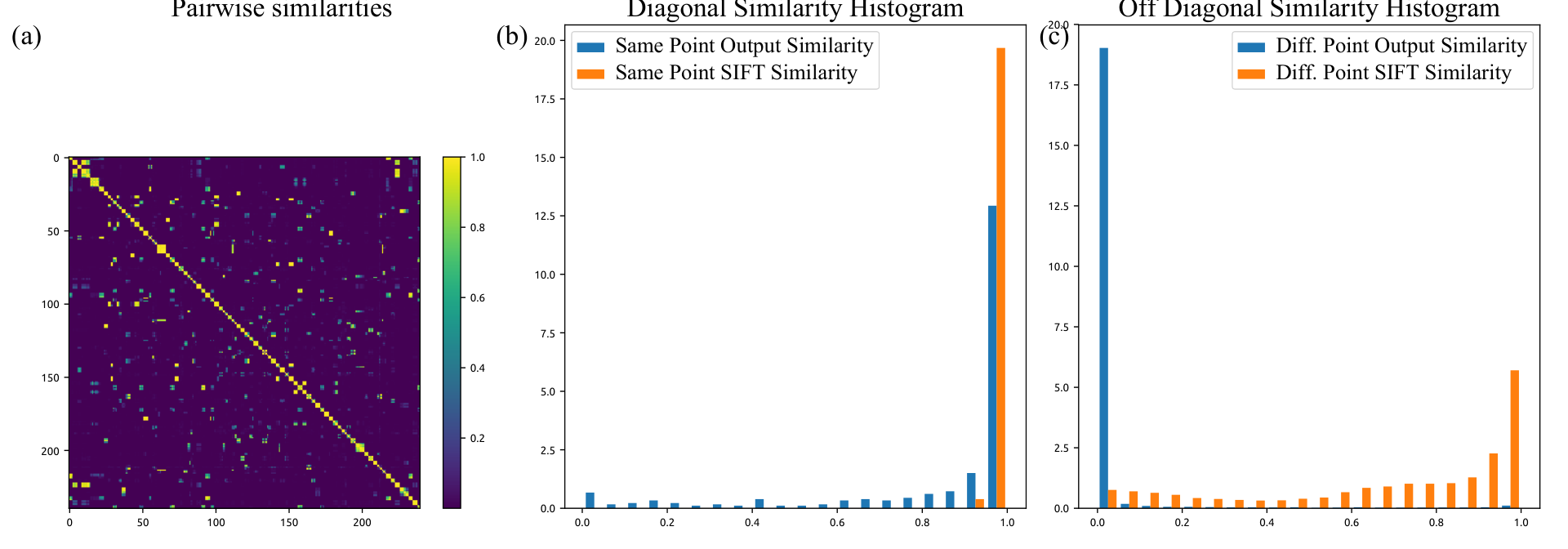
We first test our method on synthetically generated data as a simple proof of concept. To generate the data, we generate points, each with its own randomly generated descriptor. To create the graph, we generate random permutation matrices, with a noise applied to it after it is generated. We initialize the input descriptors using the true descriptor, plus some added Gaussian noise. No geometric losses were added during training for these experiments. However, the method was robust in testing with different noise functions and parameters. The normalized noisy input descriptors are our baseline - they correlate with the true values but do not preserve the structure well. However, the GCN recovered the true structure very well, as shown in Table 1. All experiments were run with a 12 layer GCN with the ReLU nonlinearity and skip connections. All were trained with the Adam optimizer kingma2014adam and a learning rate
4.2 Rome 16K Graph Dataset
We use the Rome16K dataset li2010location to test our algorithm in real world settings. Rome16K consists of 16 thousand images of various historical sites in Rome extracted from Flickr, along with the 3D structure of the sites provided by bundle adjustment. While not a standard dataset to test cycle consistency, other datasets had insufficient data to train a network on. Rome16K is typically used to test bundle adjustment methods. Therefore, to use our method, we extract image triplets and quadruplets with overlap of 80 points or more to test our algorithm, with the points established as corresponding in the given bundle adjustment output. For the initial embedding we use the original 128 dimensional SIFT descriptors, normalized to have unit norm, the calibrated x-y position, the orientation, and log scale of the SIFT feature.
For these experiments we train with the norm and geometric consistency losses. We evaluate on a test set using the ground truth adjacency matrix, which we compute from the bundle adjustment given by the Rome16K dataset. Traditional methods of evaluation use Precision and Recall, after making the labels 0 or 1. We forgo this as our method was trained to output soft labels - we in turn make the labels soft for the optimization based methods. For this method to work, we need the dimension of the embedding to be at least the number of unique points in the scene. Picking the correct number is difficult a-priori, and is a problem with all cycle consistency based methods. Here we use the ground truth dimension of the embedding to test both our method and the baselines. For implementation details, our network has 12 layers, and was trained with the Adam optimizer kingma2014adam with a learning rate of , with an exponentially decaying learning rate. We incorporate skip connections between the input, , and layers, which greatly improved training convergence and testing performance (see supplemental material).
We compare our method to spectral and optimization based baselines with different maximum iteration cutoffs. Our method is signification better than a simple spectral based optimization. Our network, though only 12 layers, has comparable accuracy to MatchALS zhou2015multi run between 25 and 50 iterations. Although our method does not outperform the Projected Gradient Descent - Doubly Stochastic (PGDDS) leonardos2016distributed method, we have significantly better run time. Additional comparisons to different iterations numbers of iterations can be found in the supplementary material.

5 Conclusion
We have shown a novel method for training feature matching using GCNs, using an unsupervised cycle consistency loss and geometric consistency losses. We have demonstrated its effectiveness on the Rome16K dataset compared to the traditional optimization based baselines on a simple GCN. For future work, we will investigate robust losses for better outlier rejection, and using higher order geometric constraints, such as the tri-focal tensor, as additional loss terms. A long term goal is to incorporate learning image level features into this pipeline. Moreover we hope to adapt this method to a distributed setting, which would be a simple extention given current approach.
Acknowledgements
Support by ARL DCIST CRA W911NF-17-2-0181, NSF-IIS-1703319, ARL RCTA W911NF-10-2-0016, ONR N00014-17-1-2093, and the Honda Research Institute is gratefully acknowledged.
References
- (1) F. Arrigoni, E. Maset, and A. Fusiello. Synchronization in the symmetric inverse semigroup. In International Conference on Image Analysis and Processing, pages 70–81. Springer, 2017.
- (2) P. W. Battaglia, J. B. Hamrick, V. Bapst, A. Sanchez-Gonzalez, V. Zambaldi, M. Malinowski, A. Tacchetti, D. Raposo, A. Santoro, R. Faulkner, et al. Relational inductive biases, deep learning, and graph networks. arXiv preprint arXiv:1806.01261, 2018.
- (3) H. Bay, T. Tuytelaars, and L. Van Gool. Surf: Speeded up robust features. In European conference on computer vision, pages 404–417. Springer, 2006.
- (4) E. Brachmann, A. Krull, S. Nowozin, J. Shotton, F. Michel, S. Gumhold, and C. Rother. Dsac-differentiable ransac for camera localization. In IEEE Conference on Computer Vision and Pattern Recognition (CVPR), volume 3, 2017.
- (5) F. J. Bremner, S. J. Gotts, and D. L. Denham. Hinton diagrams: Viewing connection strengths in neural networks. Behavior Research Methods, Instruments, & Computers, 26(2):215–218, 1994.
- (6) M. M. Bronstein, J. Bruna, Y. LeCun, A. Szlam, and P. Vandergheynst. Geometric deep learning: going beyond euclidean data. IEEE Signal Processing Magazine, 34(4):18–42, 2017.
- (7) J. Bruna, W. Zaremba, A. Szlam, and Y. LeCun. Spectral networks and locally connected networks on graphs. arXiv preprint arXiv:1312.6203, 2013.
- (8) M. Calonder, V. Lepetit, M. Ozuysal, T. Trzcinski, C. Strecha, and P. Fua. Brief: Computing a local binary descriptor very fast. IEEE Transactions on Pattern Analysis and Machine Intelligence, 34(7):1281–1298, 2012.
- (9) C. B. Choy, J. Gwak, S. Savarese, and M. Chandraker. Universal correspondence network. In Advances in Neural Information Processing Systems, pages 2414–2422, 2016.
- (10) M. Defferrard, X. Bresson, and P. Vandergheynst. Convolutional neural networks on graphs with fast localized spectral filtering. In Advances in Neural Information Processing Systems, pages 3844–3852, 2016.
- (11) M. A. Fischler and R. C. Bolles. Random sample consensus: a paradigm for model fitting with applications to image analysis and automated cartography. Communications of the ACM, 24(6):381–395, 1981.
- (12) F. Gama, G. Leus, A. G. Marques, and A. Ribeiro. Convolutional neural networks via node-varying graph filters. In 2018 IEEE Data Science Workshop (DSW), pages 1–5. IEEE, 2018.
- (13) F. Gama, A. G. Marques, A. Ribeiro, and G. Leus. Mimo graph filters for convolutional neural networks. arXiv preprint arXiv:1803.02247, 2018.
- (14) N. Hu, B. Thibert, and L. Guibas. Distributable consistent multi-graph matching. arXiv preprint arXiv:1611.07191, 2016.
- (15) D. P. Kingma and J. Ba. Adam: A method for stochastic optimization. arXiv preprint arXiv:1412.6980, 2014.
- (16) T. N. Kipf and M. Welling. Semi-supervised classification with graph convolutional networks. arXiv preprint arXiv:1609.02907, 2016.
- (17) S. Leonardos, X. Zhou, and K. Daniilidis. Distributed consistent data association. arXiv preprint arXiv:1609.07015, 2016.
- (18) Y. Li, N. Snavely, and D. P. Huttenlocher. Location recognition using prioritized feature matching. In European conference on computer vision, pages 791–804. Springer, 2010.
- (19) D. G. Lowe. Distinctive image features from scale-invariant keypoints. International journal of computer vision, 60(2):91–110, 2004.
- (20) R. Mur-Artal, J. M. M. Montiel, and J. D. Tardos. Orb-slam: a versatile and accurate monocular slam system. IEEE Transactions on Robotics, 31(5):1147–1163, 2015.
- (21) D. Pachauri, R. Kondor, and V. Singh. Solving the multi-way matching problem by permutation synchronization. In Advances in neural information processing systems, pages 1860–1868, 2013.
- (22) F. Scarselli, M. Gori, A. C. Tsoi, M. Hagenbuchner, and G. Monfardini. The graph neural network model. IEEE Transactions on Neural Networks, 20(1):61–80, 2009.
- (23) Y. Suh, K. Adamczewski, and K. Mu Lee. Subgraph matching using compactness prior for robust feature correspondence. In Proceedings of the IEEE Conference on Computer Vision and Pattern Recognition, pages 5070–5078, 2015.
- (24) R. Tron and K. Daniilidis. On the quotient representation for the essential manifold. In Proceedings of the IEEE Conference on Computer Vision and Pattern Recognition, pages 1574–1581, 2014.
- (25) R. Tron, X. Zhou, C. Esteves, and K. Daniilidis. Fast multi-image matching via density-based clustering. In Proc. IEEE Conf. Comput. Vis. Pattern Recognit., pages 4057–4066, 2017.
- (26) Q. Wang, X. Zhou, and K. Daniilidis. Multi-image semantic matching by mining consistent features. arXiv preprint arXiv:1711.07641, 2017.
- (27) Y. Wu and K. He. Group normalization. arXiv preprint arXiv:1803.08494, 2018.
- (28) K. M. Yi, E. Trulls, V. Lepetit, and P. Fua. Lift: Learned invariant feature transform. In European Conference on Computer Vision, pages 467–483. Springer, 2016.
- (29) K. M. Yi, E. Trulls, Y. Ono, V. Lepetit, M. Salzmann, and P. Fua. Learning to find good correspondences. In Proceedings of the 2018 IEEE/CVF Conference on Computer Vision and Pattern Recognition (CVPR), number CONF, 2018.
- (30) S. Zagoruyko and N. Komodakis. Learning to compare image patches via convolutional neural networks. In Proceedings of the IEEE Conference on Computer Vision and Pattern Recognition, pages 4353–4361, 2015.
- (31) X. Zhou, M. Zhu, and K. Daniilidis. Multi-image matching via fast alternating minimization. In Proceedings of the IEEE International Conference on Computer Vision, pages 4032–4040, 2015.
- (32) J.-Y. Zhu, T. Park, P. Isola, and A. A. Efros. Unpaired image-to-image translation using cycle-consistent adversarial networks. arXiv preprint, 2017.
Appendix
A. Relative Efficiency Against Optimization Based Methods
In figure 8 we show a more fine grained comparison of our algorithm to optimization based methods at different numbers of iterations. We show the mean and standard devation of the errors of all methods, testing the optimization based methods at different iterations.
B. Effect of Group Normalization
We observe that training with group normalization helps with training and generalization error, as shown in figure 9. As the Group Normalization operation is not easily parallelized across nodes in the graph, the use of Group Normalization is the main barrier to parallelization. Thus we will need to find alternative more parallelizable methods to improve generalization error for future work.