A Bayesian Framework for Persistent Homology
Abstract
Persistence diagrams offer a way to summarize topological and geometric properties latent in datasets. While several methods have been developed that utilize persistence diagrams in statistical inference, a full Bayesian treatment remains absent. This paper, relying on the theory of point processes, presents a Bayesian framework for inference with persistence diagrams relying on a substitution likelihood argument. In essence, we model persistence diagrams as Poisson point processes with prior intensities and compute posterior intensities by adopting techniques from the theory of marked point processes. We then propose a family of conjugate prior intensities via Gaussian mixtures to obtain a closed form of the posterior intensity. Finally we demonstrate the utility of this Bayesian framework with a classification problem in materials science using Bayes factors.
Keywords Bayesian inference and classification, intensity, marked Poisson point processes, topological data analysis, high entropy alloys, atom probe tomography.
1 Introduction
A crucial first step in understanding patterns and properties of a crystalline material is determining its crystal structure. For highly disordered metallic alloys, such as high entropy alloys (HEAs), atom probe tomography (APT) gives a snapshot of the local atomic environment; see Figure 1. However, APT has two main drawbacks: experimental noise and an abundance of missing data. Approximately 65% of the atoms in a sample are not registered in a typical experiment [50], and the spatial coordinates of those identified atoms are corrupted by experimental noise [42]. Understanding the atomic pattern within HEAs using an APT image requires observation of atomic cubic unit neighborhood cells under a microscope. This is problematic as APT may have a spatial resolution approximately the length of the unit cell under consideration [28, 42]. Hence, the process is unable to see the finer details of a material, rendering the determination of a lattice structure a challenging problem [55, 38]. Existing algorithms for detecting the crystal structure [13, 24, 25, 32, 43, 56] are not able to establish the crystal lattice of an APT dataset, as they rely on symmetry arguments based on identifying repeating parts of molecules. Consequently, the field of atom probe crystallography, i.e., determining the crystal structure from APT data, has emerged in recent years [21] and [43]. Algorithms in this field rely on knowing the global lattice structure a priori and aim to determine local small-scale structures within a larger sample. For some materials this information is readily known, while for others, such as HEAs, the global structure is unknown and must be inferred.
A recent work [62] proposes a machine-learning approach to classifying crystal structures of a noisy and sparse materials dataset without knowing the global structure a priori. The authors employ a convolutional neural network for classifying the crystal structure by examining a diffraction image, a computer-generated diffraction pattern. The authors suggest their method could be used to determine the crystal structure of APT data. However, the synthetic data considered in [62] is not a realistic representation of experimental APT data, where about 65% of the data is missing and furthermore corrupted by observational noise. Most importantly, their synthetic data is either sparse or noisy, not a combination of both. Herein, we consider a combination of noise and sparsity such as is the case in real APT data.


In this work, we specifically classify unit cells that are either body-centered cubic (BCC) or face-centered cubic (FCC). These lattice structures are the essential building blocks of HEAs [61] and have fundamental differences that set them apart in the case of noise-free, complete materials data. The BCC structure has a single atom in the center of the cube, while the FCC has a void in its center but has atoms on the center of the cubes’ faces, see Figure 1 (b-c). These two crystal structures are distinct when viewed through the lens of topology. Differentiating between the empty space and connectedness of these two lattice structures allows us to create an accurate classification rule. This fundamental distinction between BCC and FCC point clouds is captured well by topological methods and explains the high degree of accuracy in the classification scheme presented herein. Indeed, we offer a Bayesian classification framework for persistence homology.
Overall, topological data analysis (TDA) encompasses a broad set of techniques that explore topological structure in datasets [17, 22, 12, 59]. One of these techniques, persistent homology, associates shapes to data and summarizes salient features with persistence diagrams – multisets of points that represent homological features along with their appearance and disappearance scales [17]. Features of a persistence diagram that exhibit long persistence describe global topological properties in the underlying dataset, while those with shorter persistence encode information about local geometry and/or noise. Hence, persistence diagrams can be considered multiscale summaries of data’s shape. While there are several methods present in literature to compute persistence diagrams, we adopt geometric complexes that are typically used for applications of persistent homology to data analysis in various settings such as handwriting analysis [2], studying of brain arteries [4, 5], image analysis [7, 11, 10], neuroscience [14, 54, 3], sensor network [16, 52], protein structure [20, 31], biology [51, 39, 45], dynamical system [29], action recognition [58], signal analysis [35, 34, 47, 36], chemistry [60], genetics [26], object data [46], etc.
Researchers desire to utilize persistence diagrams for inference and classification problems. Several achieve this directly with persistence diagrams [40, 35, 6, 19, 41, 49, 9], while others elect to first map them into a Hilbert space [8, 48, 1, 57, 18]. The latter approach enables one to adopt traditional machine learning and statistical tools such as principal component analysis, random forests, support vector machines, and more general kernel-based learning schemes. Despite progress toward statistical inference, to the best of our knowledge, a full Bayesian treatment predicated upon creating posterior distributions of persistence diagrams is still absent in literature. The first Bayesian considerations in a TDA context take place in [41] where the authors discuss a conditional probability setting on persistence diagrams where the likelihood for the observed point cloud has been substituted by the likelihood for its associated topological summary.
The homological features in persistence diagrams have no intrinsic order implying they are random sets as opposed to random vectors. This viewpoint is embraced in [40] to construct a kernel density estimator for persistence diagrams. This kernel density estimator gives a sensible way to obtain priors for distributions of persistence diagrams; however, computing posteriors entirely through the random set analog of Bayes’ rule is computationally intractable in general settings [23]. Intuitively, this follows because evaluation of fixed sets in the likelihoods for parametric densities of random sets may involve a term for each possible association of input points to parameters, resulting in exponential scaling with respect to the number of parameters. To address this, we model random persistence diagrams as Poisson point processes. The defining feature of these point processes is that they are solely characterized by a single parameter known as the intensity. Utilizing the theory of marked point processes, we obtain a method for computing posterior intensities that does not require us to consider explicit maps between input diagrams and underlying parameters, alleviating the computational burden associated with deriving the posterior intensity from Bayes’ rule alone.
In particular, for a given collection of observed persistence diagrams, we consider the underlying stochastic phenomena generating persistence diagrams to be Poisson point processes with prior uncertainty captured in presupposed intensities. In applications, one may select an informative prior by choosing an intensity based on expert opinion, or alternatively choose an uninformative prior intensity when information is not available. The likelihood functions in our model represent the level of belief that observed diagrams are representative of the entire population. We build this analog using the theory of marked Poisson point processes [15]. A central idea of this paper is to utilize the topological summaries of point clouds in place of the actual point clouds. This provides a powerful tool with applications in wide ranging fields. The application considered in this paper is the classification of the crystal structure of materials, which allows scientists to predict the properties of a crystalline material. Our goal is to view point clouds through their topological descriptors as this can reveal essential shape peculiarities latent in the point clouds. Our Bayesian method adopts a substitution likelihood technique by Jeffreys in [27] instead of considering the full likelihood for the point cloud. A similar sort of discussion was considered in [41] for defining conditional probability on persistence diagrams.
Another key contribution of this paper is the derivation of a closed form of the posterior intensity, which relies on conjugate families of Gaussian mixtures. An advantage of this Gaussian mixture representation is that it allows us to perform Bayesian inference in an efficient and reliable manner. Indeed, this model can be viewed as an analog of the ubiquitous example in standard Bayesian inference where a Gaussian prior and likelihood yield a Gaussian posterior. We present a detailed example of our closed form implementation to demonstrate computational tractability and showcase its applicability by using it to build a Bayes factor classification algorithm; we test the latter in a classification problem for materials science data.
The contributions of this work are:
- 1.
Theorem 3.1, which provides the Bayesian framework for computing the posterior distribution of persistence diagrams.
- 2.
Proposition 3.1, which yields a conjugate family of priors based on a Gaussian mixture for the proposed Bayesian framework.
- 3.
A classification scheme using Bayes factors considering the posteriors of persistence diagrams and its application to a materials science problem.
This paper is organized as follows. Section 2 provides a brief overview of persistence diagrams and general point processes. Our methods are presented in Section 3. In particular, Subsection 3.1 establishes the Bayesian framework for persistence diagrams, while Subsection 3.2 contains the derivation of a closed form for a posterior distribution based on a Gaussian mixture model. A classification algorithm with Bayes factors is discussed in Section 4. To assess the capability of our algorithm, we investigate its performance on materials data in Subsection 4.1. Finally, we end with discussions and conclusions in Section 5.
2 Background
We begin by discussing preliminary definitions essential for building our model. In Subsection 2.1, we briefly review simplicial complexes and provide a formal definition for persistence diagrams (PDs). Pertinent definitions and theorems from point processes (PPs) are discussed in Subsection 2.2 .
2.1 Persistence Diagrams
We start by discussing simplices and simplicial complexes, intermediary structures for constructing PDs.
Definition 2.1.
A -dimensional collection of data is said to be geometrically independent if for any set with , the equation implies that for all
Definition 2.2.
A simplex, is a collection of geometrically independent elements along with their convex hull: . We say that the vertices span the dimensional simplex, . The faces of a simplex , are the simplices spanned by subsets of .
Definition 2.3.
A simplicial complex is a collection of simplices satisfying two conditions: (i) if , then all faces of are also in , and (ii) the intersection of two simplices in is either empty or contained in .
Given a point cloud , our goal is to construct a sequence of simplicial complexes that reasonably approximates the underlying shape of the data. We accomplish this by using the Vietoris-Rips filtration.
Definition 2.4.
Let be a point cloud in and . The Vietoris-Rips complex of is defined to be the simplicial complex satisfying if and only if . Given a nondecreasing sequence with , we denote its Vietoris-Rips filtration by .
A persistence diagram is a multiset of points in , where and each element represents a homological feature of dimension that appears at scale during a Vietoris-Rips filtration and disappears at scale . Intuitively speaking, the feature is a dimensional hole lasting for duration . Namely, features with correspond to connected components, to loops, and to voids. An example of a PD is shown in Figure 2.
2.2 Poisson Point Processes
This section contains basic definitions and fundamental theorems from PPs, primarily Poisson PPs. Detailed treatments of Poisson PPs can be found in [15] and references therein. For the remainder of this section, we take and to be a Polish space and its Borel -algebra, respectively.
Definition 2.5.
A finite point process is a pair where and is a symmetric probability measure on , where is understood to be the trivial -algebra.
The sequence defines a cardinality distribution and the measures give spatial distributions of vectors for fixed . Definition 2.5 naturally prescribes a method for sampling a finite PP: (i) determine the number of points by drawing from then, (ii) spatially distribute according to a draw from . As PPs model random collections of elements in whose order is irrelevant, any sensible construction relying on random vectors should assign equal weight to all permutations of . This is ensured by the symmetry requirement in Definition 2.5. We abuse notation and write for samples from as well as their set representations. It proves useful to describe finite PPs by a set of measures that synthesize and to simultaneously package cardinality and spatial distributions.
Definition 2.6.
Let be a finite PP. The Janossy measures are defined as the set of measures satisfying
Given a collection of disjoint rectangles , the value is the probability of observing exactly one element in each of and none in the complement of their union. For applications, we are primarily interested in Janossy measures that admit densities with respect to a reference measure on . We are now ready to describe the class of finite PPs that model PDs.
Definition 2.7.
Let be a finite measure on and . 7The finite point process is Poisson if, for all and measurable rectangles , and We call an intensity measure.
Equivalently, a Poisson PP is a finite PP with Janossy measures The intensity measure in Definition 2.7 admits a density, , with respect to some reference measure on . Notice that for all , . Elementary calculations then show . Thus, we interpret the intensity measure of a region , as the expected number of elements in that land in . The intensity measure serves as an analog to the first order moment for a random variable.
The next two definitions involve a joint PP wherein points from one space parameterize distributions for the points living in another. Consequently, we introduce another Polish space along with its Borel -algebra to serve as the mark space in a marked Poisson PP. These model scenarios in which points drawn from a Poisson PP provide a data likelihood model for Bayesian inference with PPs.
Definition 2.8.
Suppose is a function satisfying: 1) for all , is a probability measure on , and 2) for all , is a measurable function on . Then, is a stochastic kernel from to .
Definition 2.9.
A marked Poisson point process is a finite point process on such that: (i) is a Poisson PP on , and (ii) for all , measurable rectangles , , where is the set of all permutations of and is a stochastic kernel.
Given a set of observed marks it can be shown [53] that the Janossy densities for the PP induced by on given M are
| (1) |
where is the stochastic kernel for evaluated in for a fixed value of .
The following theorems allow us to construct new Poisson PPs from existing ones. Their proofs can be found in [30].
Theorem 2.1 (The Superposition Theorem).
Let be a collection of independent Poisson PPs each having intensity measure . Then their superposition given by is a Poisson PP with intensity measure .
Theorem 2.2 (The Mapping Theorem).
Let be a Poisson PP on with -finite intensity measure and let be a -algebra. Suppose is a measurable function. Write for the induced measure on given by for all . If has no atoms, then is a Poisson PP on with intensity measure .
Theorem 2.3 (The Marking Theorem).
The marked Poisson PP in Definition 2.9 has the intensity measure given by , where is the intensity measure for the Poisson PP that induces on , and is a stochastic kernel.
The final tool we need is the probability generating functional as it enables us to recover intensity measures using a notion of differentiation. The probability generating functional can be interpreted as the PP analog of the probability generating function.
Definition 2.10.
Let be a finite PP on a Polish space . Denote by the set of all functions with . The probability generating functional of denoted is given by
| (2) |
Definition 2.11.
Let be the probability generating functional given in Equation (2). The functional derivative of in the direction of evaluated at , when it exists, is given by .
It can be shown that the functional derivative satisfies the familiar product rule [33]. As is proved in [44], the intensity measure of the Poisson PP in Definition 2.7 can be obtained by differentiating , i.e., , where is the indicator function for any . Generally speaking, one obtains the intensity measure for a general point process through , but the preceding identity suffices for our purposes since we only consider point processes for which Equation (2) is defined for all bounded .
Corollary 2.1.
The intensity function for the PP whose Janossy densities are listed in Equation (1) is .
Proof.
This directly follows from writing the probability generating functional for the PP in question using its Janossy densities then applying . By Definition 2.10, linearity of the integral, and Fubini’s theorem, we have where is the probability generating functional for the PP with Janossy densities and for . One arrives at the desired result by applying the product rule for functional derivatives and the intensity retrieval property of probability generating functionals. ∎
3 Bayesian Inference
In this section, we construct a framework for Bayesian inference with PDs by modeling them as Poisson PPs. First, we derive a closed form for the posterior intensity given a PD drawn from a finite PP, and then we present a family of conjugate priors followed by an example.
3.1 Model


Given a persistence diagram , the map given by defines tilted representation of as ; see Figure 2. In the sequel, we assume all PDs are given in their tilted representations and, unless otherwise noted, abuse notation by writing and for and , respectively. We also fix the homological dimension of features in a PD by defining .
According to Bayes’ theorem, posterior density is proportional to the product of a likelihood function and a prior. To adopt Bayesian framework to PDs, we need to define two models. In particular, our Bayesian framework views a random PD as a Poisson PP equipped with a prior intensity while observed PDs are considered to be marks from a marked Poisson PP. This enables modification of the prior intensity by incorporating observed PDs, yielding a posterior intensity based on data. Some parallels between our Bayesian framework and that for random variables (RVs) are illustrated in Table 1.
| Bayesian Framework for RVs | Bayesian Framework for Random PDs | |
|---|---|---|
| Prior | Modeled by a prior density | Modeled by a Poisson PP with prior intensity |
| Likelihood | Depends on observed data | Stochastic kernel that depends on observed PDs |
| Posterior | Compute the posterior density | A Poisson PP with posterior intensity |
Let be a finite PP and consider the following:
- (M1)
For , and are independent.
- (M2)
For fixed, and some , and are independent Poisson PPs having intensity functions and , respectively.
- (M3)
For fixed, where
- (i)
is a marked Poisson PP with a stochastic kernel density .
- (ii)
and are independent finite Poisson PPs where has intensity function .
- (i)
Hereafter we abuse notation by writing for . The modeling assumption (M1) allows us to develop results independently for each homological dimension then combine them using independence. In (M2), the random persistence diagram modeled as a Poisson PP with prior intensity . There are two cases we may encounter for any point from the prior intensity due to the nature of persistence diagrams. We assign a probability function to accommodate these two possibilities. Depending upon the noise level in data, any feature in may not be represented in observations and this scenario happens with probability and we denote this case as in (M2). Otherwise a point observed with a probability of and this scenario is presented as in (M2). Consequently, the intensities of and are proportional to the intensity weighted by and respectively and the total prior intensity for is given by their sum. (M3) considers observed persistence diagram and decomposes it into two independent PDs, and . is linked to via a marked point process with likelihood defined in Equation (1), whereas the component includes any point that arises from noise or unanticipated geometry. See Figure 3 for a graphical representation of these ideas.


Theorem 3.1 (Bayesian Theorem for Persistence Diagrams).
Let be a persistence diagram modeled by a Poisson PP as in (M2). Suppose and have prior intensities and , respectively. Consider independent samples from the point process that characterizes the persistence diagram of (M3) and denote where for all . Moreover, is the likelihood associated for the stochastic kernel between and , and is the intensity of as defined in (M3). Then, the posterior intensity of given is
| (3) |
The proof of Theorem 3.1 can be found in the appendix. One important point about the above theorem is that, instead of relying on a likelihood function for the point cloud data, our Bayesian model considers the likleihood for the persistence diagram generated by the observed point cloud data at hand. This is analogous to the idea of substitution likelihood by Jeffreys in [27].
3.2 A Conjugate Family of Prior Intensities: Gaussian Mixtures
This section focuses on constructing a family of conjugate prior intensities, i.e., a collection of priors that yield posterior intensities of the same form when used in Equation (3). Exploiting Theorem 3.1 with Gaussian mixture prior intensities, we obtain Gaussian mixture posterior intensities. As PDs are stochastic point processes on the space , not , we consider a restricted Gaussian density restricted to . Namely, for a Gaussian density on , , with mean and covariance matrix , we restrict the Gaussian density on as
| (4) |
where is the indicator function of the wedge . ‘
Consider a random persistence diagram as in (M2) and a collection of observed PDs that are independent samples from Poisson PP characterizing the PD in (M3). We denote . Below we specialize (M2) and (M3) so that applying Theorem 3.1 to a mixed Gaussian prior intensity yields a mixed Gaussian posterior:
- (M2′)
, where and are independent Poisson PPs with intensities and , respectively, with
(5) where is the number of mixture components.
- (M3′)
where
- (i)
the marked Poisson PP has density given by
(6) - (ii)
and are independent finite Poisson PPs and has intensity function given below.
(7) where is the number of mixture components.
- (i)
Proposition 3.1.
Suppose that the assumptions (M1),(M2′), and (M3′) hold; then, the posterior intensity of Equation (3) in Theorem 3.1 is a Gaussian mixture of the form
| (8) |
The proof of Proposition 3.1 follows from well known results about products of Gaussian densities given below; for more details, the reader may refer to [37] and references therein.
Lemma 3.1.
For matrices , with and positive definite ,and a vector ,
, where and .
Proof of Proposition 3.1.
Using Lemma 3.1, we first derive by observing that, in our model, and . By typical matrix operations we obtain, , and . Hence the numerator and denominator of the second term in Equation (3), , and respectively, yield
where the bracketed expression is the definition of . ∎
3.2.1 Example
Here, we present a detailed example of computing the posterior intensity according to Equation (8) for a range of parametric choices. Reproducing these results, the interested reader may download our R-package BayesTDA. We consider circular point clouds often associated with periodicity in signals [35] and focus on estimating homological features with as they correspond to 1-dimensional holes, which describe the prominent topological feature of a circle. Precisely our goals are to: (i) illustrate posterior intensities and draw analogies to standard Bayesian inference; (ii) determine the relative contributions of the prior and observed data to the posterior; and (iii) perform sensitivity analysis.
.
| Informative Prior | |||
|---|---|---|---|
| Weakly informative Prior | |||
| Unimodal Uninformative Prior | |||
| Bimodal Uninformative Prior |
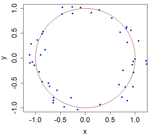
We start by considering a Poisson PP with prior intensity that has the Gaussian mixture form given in (M2′). We take into account four types of prior intensities: (i) informative, (ii) weakly informative, (iii) unimodal uninformative, and (iv) bimodal uninformative; see Figures 5–7 (a), (d), (g), (j), respectively. We use one Gaussian component in each of the first three priors as the underlying shape has single dimensional feature and two for the last one to include a case where we have no information about the cardinality of the underlying true diagram. The parameters of the Gaussian mixture density in Equation (5) used to compute these prior intensities are listed in Table 2. To present the intensity maps uniformly throughout this example while preserving their shapes, we divide the intensities by their corresponding maxima. This ensures all intensities are on a scale from to , and we call it the scaled intensity. The observed PDs are generated from point clouds sampled uniformly from the unit circle and then perturbed by varying levels of Gaussian noise; see Figure 4 wherein we present three point clouds sampled with Gaussian noise having variances , , and , respectively. Consequently, these point clouds provide persistence diagrams for , which are considered as independent samples from Poisson point process , exhibiting distinctive characteristics such as only one prominent feature with high persistence and no spurious features (Case-I), one prominent feature with high persistence and very few spurious features (Case-II), and one prominent feature with medium persistence and more spurious features (Case-III).
 Case-I
 Case-II
 Case-III
Parameters for (M3′) in Equation (6) and (7). We set the weight and mean of the Gaussian component, and respectively for all of the cases. The first row corresponds to parameters in the functions characterizing that are used in computing the posterior depicted in the first column of Figure 8. The second row corresponds to analogous parameters that are used in computing the posterior depicted in the second columns of Figures 5–8. Similarly, the third row corresponds to parameters in the functions characterizing used for computing the posterior presented in the third columns of Figures 5–8.
| Case-I | Case-II | Case-III | Case-IV |
|---|---|---|---|
For each observed PD, persistence features are presented as green dots overlaid on their corresponding posterior intensity plots. For Cases-I-III, we set the probability of the event that a feature in appears in to , i.e., any feature in is certainly observed through a mark in , and later in Case-IV, we decrease to while keeping all other parameters the same for the sake of comparison. The choice of anticipates that any feature has equal probability to appear or disappear in the observation and in turn provides further intuition about the contribution of prior intensities to the estimated posteriors. We observe that in all cases, the posterior estimates the dimensional hole; however, with different uncertainty each time. For example, for the cases where the data are trustworthy, expressed by a likelihood with tight variance, or in the case of an informative prior, the posterior accurately estimates the dimensional hole. In contrast, when the data suffer from high uncertainty and the prior is uninformative, then the posterior offers a general idea that the true underlying shape is a circle, but the exact estimation of the 1-dimensional hole is not accurate. We examine the cases below.


Case-I: We consider informative, weakly informative, unimodal uninformative and bimodal uninformative prior intensities as presented in Figure 5 (a), (d), (g) and (j) respectively to compute corresponding posterior intensities. The prior intensities parameters are listed in Table 2. The observed PD is obtained from the point cloud in Figure 4 (left). The parameters associated to the observed PD are listed in Table 3. For the observed PD arising from data with very low noise, we observe that the posterior computed from any of the priors predicts the existence of a one dimensional hole accurately. Firstly, with a low variability in observed persistence diagram , the posterior intensities estimate the hole with high certainty (Figure 5 (b), (e), (h) and (k) respectively). Next, to determine the effect of observed data on the posterior, we increase the variance of the observed PD component , which consists of features in observed PDs that are associated to the underlying prior. Here, we observe that the posterior intensities still estimate the hole accurately due to the trustworthy data; this is evident in Figure 5 (c), (f), (i) and (l). In Figure 5, the posteriors in (b), (e), (h), and (k) have lower variance around the 1-dimensional feature in comparison to (c), (f), (i), and (l) respectively.


.
| Case-I | Case-II | Case-III | |
|
Informative |
![[Uncaptioned image]](1901.02034v2/Fig_7_a_diff_r.png)
|
![[Uncaptioned image]](1901.02034v2/Fig_7_b_r.png)
|
![[Uncaptioned image]](1901.02034v2/Fig_7_c_r.png)
|
|
Weakly Informative |
![[Uncaptioned image]](1901.02034v2/Fig_7_d_r.png)
|
![[Uncaptioned image]](1901.02034v2/Fig_7_e_r.png)
|
![[Uncaptioned image]](1901.02034v2/Fig_7_f_r.png)
|
|
Unimodal Uninformative |
![[Uncaptioned image]](1901.02034v2/Fig_7_g_r.png)
|
![[Uncaptioned image]](1901.02034v2/Fig_7_h_diff_r.png)
|
![[Uncaptioned image]](1901.02034v2/Fig_7_i_r.png)
|
|
Bimodal Uninformative |
![[Uncaptioned image]](1901.02034v2/Fig_7_j_diff_r.png)
|
![[Uncaptioned image]](1901.02034v2/Fig_7_k_r.png)
|
![[Uncaptioned image]](1901.02034v2/Fig_7_l_r.png)
|
Case-II: Here, we consider all four priors as in Case-I (see Figure 6 (a), (d), (g) and (j)). The point cloud in Figure 4 (center) is more perturbed around the unit circle than that of Case-I (Gaussian noise with variance ). Due to this, the associated PD exhibits spurious features. The parameters used for this case are listed in Table 3. We compute the posterior intensities for each type of prior. First, to illustrate the posterior intensity and check the capability of detecting the dimensional feature, we use moderate noise for the observed PD . The results are presented in Figure 6 (b), (e), (h), and (k); overall, the posteriors estimate the prominent feature with different variances in their respective posteriors. Next, to illustrate the effect of observed data on the posterior, we increase the variance of . According to our Bayesian model, the persistence diagram component contains features that are not associated with , so increasing yields that every observed point is linked to , and therefore one may expect to observe increased intensity skewed towards the spurious points that arise from noise. Indeed, posterior intensities with weakly informative, unimodal uninformative, and bimodal uninformative priors exhibit the skewness toward the spurious point in Figure 6 (f), (i) and (l) respectively, but this is not the case when an informative prior is used. In (f), we observe increased intensity skewing towards the spurious points, and in (i) and (l) the intensity appears to be bimodal with two modes – one at the prominent and other at the spurious point. For the bimodal uninformative prior since one mode is located close to the spurious point in the observed PD, we observe higher intensity for that mode in the posterior (Figure 6 (l)) with another mode estimating the prominent feature.
Case-III: We again consider the four types of priors here. The observed PD constructed from the point cloud in Figure 4 (right). The point cloud has Gaussian noise with variance and due to the high noise level in sampling relative to the unit circle, the associated PD exhibits one prominent feature and several spurious features. We repeat the parameter choices as in Case-I for the variances of observed PD. For the choice of and , the posteriors computed from all of the four priors are able to detect the difference between the one prominent and other spurious points. We increase the variance of to determine the effect of observed PD on the posterior and we observe that only the posterior intensity from informative prior has evidence of the hole (Figure 7(c)). For the weakly informative and uninformative priors, while the posteriors in (f), (i) and (l) may not detect the hole clearly, in (f) we observe a mode with higher variance and in (i) and (l), a tail towards the high persistence point implying presence of a hole. It should be noted that with the informative prior the posterior intensity identifies the hole closer to the mode of the prior as we increase the variance in .
Case-IV: Lastly, in this case we concentrate on the effect of . The rest of the parameters used for this case remain the same and are listed in Table 3. We decrease to to model the scenario that a feature in has equal probability to appear or vanish in observed . The columns of Figure 8 correspond to the parameters of the observed persistence diagram used in computing the posteriors depicted in the third column of Figure 5, third column of Figure 6, and second column of Figure 7 respectively. By comparing them with their respective cases, we notice a change in the intensity level in all of these due to the first term of the posterior intensity on the right hand side of Equation (8). Comparing with the respective figures in Case-I, we observe that the posterior intensities are estimating the hole with higher variability for the weakly informative and unimodal uninformative priors. For bimodal prior, we observe bimodality in the posterior. Next for Case-II, the existence of a hole is evident for informative and weakly informative priors with higher uncertainty when compared to their previous cases. The unimodal and bimodal uninformative priors lead to bimodal and trimodal posteriors, respectively. We observe that the posterior resembles the prior intensity more closely when we compare them to respective figures in Case-III. One can especially see this with the informative, weakly informative and bimodal uninformative priors, which have significantly increased intensities at the location of the modes of prior.
4 Classification
The Bayesian framework introduced in this paper allows us to explicitly compute the posterior intensity of a PD given data and prior knowledge. This lays the foundation for supervised statistical learning methods in classification. In this section, we build a Bayes factor classification algorithm based on notions discussed in Section 3 and then apply it on materials data, in particular, on measurements for spatial configurations of atoms.
We commence our classification scheme with a persistence diagram belonging to an unknown class. We assume that is sampled from a Poisson point process in with the prior intensity having the form in (M2′). Consequently, its probability density has the form
| (9) |
where , with probability as in (M2′). Next suppose we have two training sets and from two classes of random diagrams and , respectively. The likelihood densities of respective classes take the form of Equation (6). We then follow Equation (8) to obtain the posterior intensities of given the training sets and from the prior intensities and likelihood densities. In particular, the corresponding posterior probability density of given the training set is
| (10) |
and the posterior probability density given is given by an analogous expression. The Bayes factor defined by
| (11) |
provides the decision criterion for assigning to either or . More specifically, for a threshold , implies that belongs to and implies otherwise. We summarize this scheme in Algorithm 1 .
4.1 Atom Probe Tomography Data
Our goal in this section is to use Algorithm 1 to classify the crystal lattice of a noisy and sparse materials dataset, where the unit cells are either Body centered cubic (BCC) or Face centered cubic (FCC); recall Figure 1. The BCC structure has a single atom in the center of the cube, while the FCC has a void in its center but has atoms on the centers of the cubes’ faces (Figure 1 (b-c)). However, sparsity and noise do not allow the crystal structure to be revealed. For high-entropy alloys, our object of interest, APT, provides the best atomic level characterization possible. Due to the sparsity and noise in the resulting data, there are only a few algorithms for successfully determining the crystal structure; see [21, 43]. These algorithms, designed for APT data, rely on knowing the global structure a priori (which is not the case for High Entropy Alloys (HEAs)) and seek to discover small-scale structure within a sample.
Bypassing this restriction, the neural network architecture of [62] provides a way to classify the crystal structure of a noisy or sparse dataset by looking at a diffraction image. However, the authors use a test data case with very low noise or sparsity, but not both cases together, which is the representative case of the APT data. The algorithm is also not publicly available, so a side by side comparison of our method with theirs using HEAs is not feasible.
It is natural to consider persistence diagrams in this setting because they distill salient information about the materials patterns with respect to connectedness and empty space (holes) within cubic unit cells, i.e we can differentiate between atomic unit cells by examining their homological features. In particular, after storing both types of spatial configurations as point clouds, we compute their Rips filtrations (see Section 2), collecting resultant 1-dimensional homological features into PDs; see Figure 9. The data set had 200 diagrams from each class. To perform classification with Algorithm 1, we started by specifying priors for each class, and . Two scenarios were considered, namely using separate priors (Prior-1 in Table 4) and the same prior (Prior-2 in Table 4) for both BCC and FCC classes. In particular, for Prior-1 we superimpose 50 PDs from each class and find the highly clustered areas by using K-means clustering. The centers of the clusters from K-means are then used as the means in Gaussian mixture priors; see Eqn. (8). In this manner, we produce different priors for BCC and FCC classes. On the other hand for Prior-2 we choose a flat prior with higher variance level than that of Prior-1 for both of the classes. The parameters for these two prior intensities are in Table 4. For all cases, we set and . We chose a relatively high weight for because the nature of the data implied that extremely low persistence holes were rare events arising from noise. To perform 10-fold cross validation, we partitioned PDs from both classes into training and test sets. During each fold, we took the training sets from each class, and , and input them into Algorithm 1 as and , respectively. Next, we computed the Bayes factor for each diagram in the test sets. After this, we used the Bayes factors to construct receiver operating characteristic (ROC) curves and computed the resulting areas under the ROC curves (AUCs) . Finally, we used the AUCs from 10-fold cross validation to build a bootstrapped distribution by resampling 2000 times. Information about these bootstrapped distributions is summarized in Table 4, which shows our scoring method almost perfectly distinguishes between the BCC and FCC classes using the Bayesian framework of Section 3. Also, it exemplifies the robustness of our algorithm as two different types of priors produce near perfect accuracy.


Parameters for the prior intensities used in cross-validation of materials science data. Each prior is indexed by its corresponding class for Prior-1 or in the case of the Prior-2. The summary of AUCs across 10-folds for materials science data after scoring with Algorithm 1 is presented in the last three columns.
| Priors | Parameters for Prior Intensities | Summary of AUC | ||||||||||||||
|---|---|---|---|---|---|---|---|---|---|---|---|---|---|---|---|---|
| 5th percentile | Mean | 95th percentile | ||||||||||||||
| Prior-1 |
|
|
|
|||||||||||||
|
|
|
||||||||||||||
| Prior-2 | (1,1) | 20 | 1 | 0.94 | ||||||||||||
5 Discussion and Conclusions
This work is the first approach to introduce a Bayesian framework for persistent homology. This toolbox will give the opportunity to an expert to incorporate their prior belief about the data as well as analyze the data using topological data analysis methods. To that end, we introduce point processes to model random persistence diagrams. Indeed, we incorporate the prior uncertainty by modeling persistence diagrams as Poisson point processes and noisy observations of persistence diagrams as marked Poisson PP to model the level of confidence that observations are representatives of the ground truth. Considering a Poisson point process, one needs to focus on the intensity of the random process. Adapting a prior intensity and a pertinent likelihood, we prove that a posterior intensity can be retrieved. It should be noted that our Bayesian model considers persistence diagrams, which are summaries of the data at hand, for defining a substitution likelihood rather than using the underlying point cloud data. This does not adhere to a strict Bayesian viewpoint, as we model the behavior of the persistence diagrams without considering the underlying data (materials data in our example) used to create it; however, our paradigm incorporates prior knowledge and observed data summaries to create posterior probabilities, analogous to the notion of substitution likelihood detailed in [27]. The general relationship between the likelihood models related to point cloud data and those of their corresponding persistence diagrams remains an important open problem. Furthermore we show that using Gaussian mixture conjugate family of priors. A detailed example is presented to demonstrate posterior intensities for several interesting instances resulted from varying parameters of the model. We establish evidence that our Bayesian framework offers update of prior uncertainty in the light of new evidence in a similar way as the standard Bayesian for random variables. Thus, the Bayesian inference developed here can be reliably used for machine learning and data analysis techniques directly on the space of PDs. Indeed a classification algorithm is derived and successfully applied on materials science data to assess the capability of our Bayesian framework.
Appendix A-Proof of Theorem 3.1
Proof.
By Theorem 2.1, we decompose to write
| (12) |
where the second equality follows because is independent of . Theorem 2.1 allows us to express as the average of intensity functions for , where the are independent and equal in distribution to . That is, , and by conditioning we have,
| (13) |
So to expand Equation (12) it suffices to compute for fixed . First, we express the finite PP as a marked Poisson PP. To this end, we adopt a construction from [53], the augmented space , where is a dummy set used for labeling points in . Next, we define the random set, such that
| (14) |
One can observe that is the superposition of two marked Poisson PPs and , taking values in and , respectively. Moreover, it directly follows from and that has marginal intensity function on and stochastic kernel density while shows that has marginal intensity function on with stochastic kernel density . By Theorem 2.3, the intensity functions for and are and , respectively. Hence, applying Theorem 2.1 to Equation (14) reveals that the intensity function for , , is given by
| (15) |
Let , be the projections of onto its first and second coordinates, respectively. It immediately follows from Theorem 2.2 that is a Poisson PP on since it is the image of under a projection. Therefore, by treating the first coordinates of as marks, we may express as a marked Poisson PP having intensity function on and stochastic kernel density from to . Another application of Theorem 2.3 then implies
| (16) |
From Equations (15) and (16), we obtain the identity
| (17) |
Equation (17) describes the probability density of at for fixed. Substituting Equation (17) for the Janossy density in Equation (1) and applying Corollary 2.1 gives the intensity function for the point process whenever for any ,
| (18) |
. Thus,
whenever , from which we conclude a.s. . Hence, restricting Equation (18) to yields
| (19) |
Notice that is the same PP as . Theorems 2.2 and 2.3 imply that is a Poisson PP, and is a Poisson PP by (M3), so by Theorem 2.1, where by Theorem 2.3. Employing Equation (19) one gets that
| (20) |
which proves Theorem 3.1 after substituting into Equation (12). ∎
Acknowledgments
Research has been partially funded by the Army Research Office, W911NF-17-1-0313, the National Science Foundation, MCB-1715794, and DMS-1821241, and Thor Industries/Army Research Lab, W911NF-17-2-0141.
References
- [1] H. Adams and et. al., Persistence images: A stable vector representation of persistent homology, Journal of Machine Learning Research, 18 (2017), pp. 218–252, http://jmlr.org/papers/v18/16-337.html.
- [2] A. Adcock, E. Carlsson, and G. Carlsson, The ring of algebraic functions on persistence bar codes, Homology, Homotopy and Applications, 18 (2016), pp. 381–402, https://doi.org/10.4310/HHA.2016.v18.n1.a21.
- [3] A. Babichev and Y. Dabaghian, Persistent memories in transient networks, Emergent Complexity from Nonlinearity, in Physics, Engineering and the Life Sciences, 191 (2017), pp. 179–188.
- [4] P. Bendich, J. S. Marron, E. Miller, A. Pieloch, and S. Skwerer, Persistent homology analysis of brain artery trees, The Annals of Applied Statistics, 10 (2016), pp. 198–218, https://doi.org/10.1214/15-AOAS886.
- [5] C. Biscio and J. Møller, The accumulated persistence function, a new useful functional summary statistic for topological data analysis, with a view to brain artery trees and spatial point process applications, Journal of Computational and Graphical Statistics, (2019), pp. 1537–2715, https://doi.org/10.1080/10618600.2019.1573686.
- [6] O. Bobrowski, S. Mukherjee, and J. E. Taylor, Topological consistency via kernel estimation, Bernoulli, 23 (2017), pp. 288–328, https://doi.org/10.3150/15-BEJ744.
- [7] T. Bonis, M. Ovsjanikov, S. Oudot, and F. Chazal, Persistence-based pooling for shape pose recognition, in Computational Topology in Image Context, ed. A Bac, JL Mari, New York: Springer, 2016, pp. 19–29.
- [8] P. Bubenik, Statistical topological data analysis using persistence landscapes, Journal of Machine Learning Research, 16 (2015), pp. 77–102, http://jmlr.org/papers/v16/bubenik15a.html.
- [9] P. Bubenik, The persistence landscape and some of its properties. arXiv 1810.04963, 2018, https://arxiv.org/abs/1810.04963.
- [10] G. Carlsson, T. Ishkhanov, V. D. Silva, and A. Zomorodian, On the local behavior of spaces of natural images, International Journal of Computer Vision, 76 (2008), pp. 1–12.
- [11] M. Carrière, S. Y. Oudot, and M. Ovsjanikov, Stable topological signatures for points on 3D shapes, Computer Graphics Forum, 34 (2015), pp. 1–12.
- [12] F. Chazal and B. Michel, An introduction to topological data analysis: fundamental and practical aspects for data scientists. arXiv:1710.04019, 2017, https://arxiv.org/abs/1710.04019.
- [13] J. Chisholm and S. Motherwell, A new algorithm for performing three-dimensional searches of the cambridge structural database, Journal of applied crystallography, 37 (2004), pp. 331–334.
- [14] M. K. Chung, J. L. Hanson, J. Ye, R. J. Davidson, and S. D. Pollak, Persistent homology in sparse regression and its application to brain morphometry, IEEE Transactions on Medical Imaging, 34 (2015), pp. 1928–1939.
- [15] D. J. Daley and D. Vere-Jones, An introduction to the theory of point processes. Vol. I, Probability and its Applications (New York), Springer-Verlag, New York, second ed., 2003.
- [16] P. Dłotko, R. Ghrist, M. Juda, and M. Mrozek, Distributed computation of coverage in sensor networks by homological methods, Applicable Algebra in Engineering, Communication and Computing, 23 (2012), pp. 29–58.
- [17] H. Edelsbrunner, Computational topology : an introduction, American Mathematical Society, Providence, R.I, 2010.
- [18] B. D. Fabio and M. Ferri, Comparing persistence diagrams through complex vectors, in International Conference on Image Analysis and Processing, 2015, pp. 294–305, https://doi.org/10.1007/978-3-319-23231-7_27.
- [19] B. T. Fasy, F. Lecci, A. Rinaldo, L. Wasserman, S. Balakrishnan, and A. Singh, Confidence sets for persistence diagrams, The Annals of Statistics, 42 (2014), pp. 2301–2339, https://doi.org/10.1214/14-AOS1252.
- [20] M. Gameiro, Y. Hiraoka, S. Izumi, M. Kramar, K. Mischaikow, and V. Nanda, A topological measurement of protein compressibility, Japan Journal of Industrial and Applied Mathematics, 32 (2015), pp. 1 – 17.
- [21] B. Gault, M. P. Moody, J. Cairney, and S. Ringer, Atom probe crystallography, Materials Today, 15 (2012), pp. 378–386.
- [22] R. Ghrist, Barcodes: The persistent topology of data, Bulletin of the American Mathematical Society, 45 (2008), pp. 61–75, https://doi.org/10.1090/S0273-0979-07-01191-3.
- [23] I. R. Goodman, Mathematics of Data Fusion, Springer Netherlands, Dordrecht, 1997.
- [24] D. Hicks, C. Oses, E. Gossett, G. Gomez, R. H. Taylor, C. Toher, M. Mehl, O. Levy, and S. Curtarolo, Aflow-sym: platform for the complete, automatic and self-consistent symmetry analysis of crystals, Acta Crystallographica Section A: Foundations and Advances, 74 (2018), pp. 184–203.
- [25] J. D. Honeycutt and H. C. Andersen, Molecular dynamics study of melting and freezing of small lennard-jones clusters, Journal of Physical Chemistry, 91 (1987), pp. 4950–4963.
- [26] D. P. Humphreys, M. R. McGuirl, M. Miyagi, and A. J. Blumberg, Fast estimation of recombination rates using topological data analysis, GENETICS, (2019), https://doi.org/10.1534/genetics.118.301565.
- [27] H. Jeffreys, Theory of Probability, Clarendon Press, 1961.
- [28] T. F. Kelly, M. K. Miller, K. Rajan, and S. P. Ringer, Atomic-scale tomography: A 2020 vision, Microscopy and Microanalysis, 19 (2013), pp. 652–664.
- [29] F. A. Khasawneh and E. Munch, Chatter detection in turning using persistent homology, Mechanical Systems and Signal Processing, 70–71 (2016), pp. 527 – 541.
- [30] J. F. C. Kingman, Poisson processes, Clarendon Press, Oxford, 1993.
- [31] G. Kusano, K. Fukumizu, and Y. Hiraoka, Persistence weighted gaussian kernel for topological data analysis, Proceedings of the 33 rd International Conference on Machine Learning, 48 (2016), pp. 2004–2013.
- [32] P. Larsen, S. Schmidt, and J. Schiøtz, Robust structural identification via polyhedral template matching, Modelling and Simulation in Materials Science and Engineering, 24 (2016), p. 055007.
- [33] R. Mahler, Statistical multisource-multitarget information fusion, Artech House, Boston, 2007.
- [34] A. Marchese and V. Maroulas, Topological learning for acoustic signal identification, in 2016 19th International Conference on Information Fusion (FUSION), July 2016, pp. 1377–1381.
- [35] A. Marchese and V. Maroulas, Signal classification with a point process distance on the space of persistence diagrams, Advances in Data Analysis and Classification, 12 (2018), pp. 657–682, https://doi.org/10.1007/s11634-017-0294-x.
- [36] A. Marchese, V. Maroulas, and J. Mike, K-means clustering on the space of persistence diagrams, in Wavelets and Sparsity XVII, vol. 10394, International Society for Optics and Photonics, 2017, p. 103940W.
- [37] V. Maroulas and A. Nebenführ, Tracking rapid intracellular movements: a Bayesian random set approach, The Annals of Applied Statistics, 9 (2015), pp. 926–949, https://doi.org/10.1214/15-AOAS819.
- [38] N. W. McNutt, O. Rios, V. Maroulas, and D. J. Keffer, Interfacial Li-ion localization in hierarchical carbon anodes, Carbon, 111 (2017), pp. 828–834, https://doi.org/10.1016/j.carbon.2016.10.061.
- [39] J. Mike, C. D. Sumrall, V. Maroulas, and F. Schwartz, Nonlandmark classification in paleobiology: computational geometry as a tool for species discrimination, Paleobiology, 42 (2016), pp. 696–706.
- [40] J. L. Mike and V. Maroulas, Nonparametric estimation of probability density functions of random persistence diagrams. arXiv:1803.02739v2, 2018, https://arxiv.org/abs/1803.02739.
- [41] Y. Mileyko, S. Mukherjee, and J. Harer, Probability measures on the space of persistence diagrams, Inverse Problems, 27 (2011), p. 124007, https://doi.org/10.1088/0266-5611/27/12/124007.
- [42] M. K. Miller, T. Kelly, K. Rajan, and S. Ringer, The future of atom probe tomography, Materials Today, 15 (2012), pp. 158–165, https://doi.org/10.1016/S1369-7021(12)70069-X.
- [43] M. P. Moody, B. Gault, L. Stephenson, R. K. Marceau, R. Powles, A. Ceguerra, A. Breen, and S. P. Ringer, Lattice rectification in atom probe tomography: Toward true three-dimensional atomic microscopy, Microscopy and Microanalysis, 17 (2011), pp. 226–239.
- [44] J. Moyal, The General Theory of Stochastic Population Processes, Acta Mathematica, 108 (1962), pp. 1–31, https://doi.org/10.1007/BF02545761.
- [45] M. M. P. Nicolau, A. J. Levine, and G. E. Carlsson, Topology based data analysis identifies a subgroup of breast cancers with a unique mutational profile and excellent survival., Proceedings of the National Academy of Sciences, 108 (2011), pp. 7265–70.
- [46] V. Patrangenaru, P. Bubenik, R. L. Paige, and D. Osborne, Topological data analysis for object data, arXiv:1804.10255, (2018).
- [47] C. M. M. Pereira and R. F. Mello, Persistent homology for time series and spatial data clustering, Expert Systems with Applications, 42 (2015), pp. 6026–6038.
- [48] J. Reininghaus, S. Huber, U. Bauer, and R. Kwitt, A stable multi-scale kernel for topological machine learning, in The IEEE Conference on Computer Vision and Pattern Recognition (CVPR), July 2015, pp. 4741–4748, https://doi.org/10.1109/CVPR.2015.7299106.
- [49] A. Robinson and K. Turner, Hypothesis testing for topological data analysis, Journal of Applied and Computational Topology, 1 (2017), pp. 241–261, https://doi.org/10.1007/s41468-017-0008-7.
- [50] L. Santodonato and et. al., Deviation from high-entropy configurations in the atomic distributions of a multi-principal-element alloy, Nature communications, 6 (2015), p. 5964, https://doi.org/10.1038/ncomms6964.
- [51] I. Sgouralis, A. Nebenführ, and V. Maroulas, A Bayesian topological framework for the identification and reconstruction of subcellular motion, SIAM Journal on Imaging Sciences, 10 (2017), pp. 871–899, https://doi.org/10.1137/16M1095755.
- [52] V. D. Silva and R. Ghrist, Coverage in sensor networks via persistent homology, Algebraic and Geometric Topology, 7 (2007), pp. 339–358, https://doi.org/10.2140/agt.2007.7.339.
- [53] S. S. Singh, B. Vo, A. Baddeley, and S. Zuyev, Filters for spatial point processes, SIAM Journal on Control and Optimization, 48 (2009), pp. 2275––2295, https://doi.org/10.1137/070710457.
- [54] A. E. Sizemore, J. E. Phillips-Cremins, R. Ghrist, and D. S. Bassett, The importance of the whole: Topological data analysis for the network neuroscientist, Network Neuroscience, (2018), https://doi.org/10.1162/netn_a_00073.
- [55] A. Spannaus, V. Maroulas, D. Keffer, and K. J. Law, Bayesian point set registration, in 2017 Matrix Annals, Springer, 2017.
- [56] A. Togo and I. Tanaka, Spglib : a software library for crystal symmetry search, arXiv preprint arXiv:1808.01590, (2018).
- [57] K. Turner, S. Mukherjee, and D. M. Boyer, Persistent homology transform for modeling shapes and surfaces, Information and Inference: A Journal of the IMA, 3 (2014), pp. 310–344, https://doi.org/10.1093/imaiai/iau011.
- [58] V. Venkataraman, K. N. Ramamurthy, and P. Turaga, Persistent homology of attractors for action recognition, in 2016 IEEE International Conference on Image Processing (ICIP), 2016, pp. 4150––4154, https://doi.org/10.1109/ICIP.2016.7533141.
- [59] L. Wasserman, Topological data analysis, Annual Review of Statistics and Its Application, 5 (2018), pp. 501–532.
- [60] K. Xia, X. Feng, Y. Tong, and G. W. Wei, Persistent homology for the quantitative prediction of fullerene stability, Journal of Computational Chemistry, 36 (2014), pp. 408–422, https://doi.org/10.1002/jcc.23816.
- [61] Y. Zhang, T. Zuo, Z. Tang, M. Gao, K. Dahmen, P. Liaw, and Z. Lu, Microstructures and properties of high-entropy alloys, Progress in Materials Science, 61 (2014).
- [62] A. Ziletti, D. Kumar, M. Scheffler, and M. Ghiringhelli, Insightful classification of crystal structures using deep learning, Nature communications, 9 (2018), p. 2775, https://doi.org/10.1038/s41467-018-05169-6.