A Scale-invariant Generalization of the Rényi Entropy,
Associated Divergences and their Optimizations
under Tsallis’ Nonextensive Framework
Abstract
Entropy and relative or cross entropy measures are two very fundamental concepts in information theory and are also widely used for statistical inference across disciplines. The related optimization problems, in particular the maximization of the entropy and the minimization of the cross entropy or relative entropy (divergence), are essential for general logical inference in our physical world. In this paper, we discuss a two parameter generalization of the popular Rényi entropy and associated optimization problems. We derive the desired entropic characteristics of the new generalized entropy measure including its positivity, expandability, extensivity and generalized (sub-)additivity. More importantly, when considered over the class of sub-probabilities, our new family turns out to be scale-invariant; this property does not hold for most existing generalized entropy measures. We also propose the corresponding cross entropy and relative entropy measures and discuss their geometric properties including generalized Pythagorean results over -convex sets. The maximization of the new entropy and the minimization of the corresponding cross or relative entropy measures are carried out explicitly under the non-extensive (‘third-choice’) constraints given by the Tsallis’ normalized -expectations which also correspond to the -linear family of probability distributions. Important properties of the associated forward and reverse projection rules are discussed along with their existence and uniqueness. In this context, we have come up with, for the first time, a class of entropy measures – a subfamily of our two-parameter generalization – that leads to the classical (extensive) exponential family of MaxEnt distributions under the non-extensive constraints; this discovery has been illustrated through the useful concept of escort distributions and can potentially be important for future research in information theory. Other members of the new entropy family, however, lead to the power-law type generalized -exponential MaxEnt distributions which is in conformity with Tsallis’ nonextensive theory. Therefore, our new family indeed provides a wide range of entropy and associated measures combining both the extensive and nonextensive MaxEnt theories under one umbrella.
Keywords: Entropy; Maximum entropy (MaxEnt) distribution; Cross-entropy minimization; Rényi entropy; Relative entropy; Non-extensive constraints; Logarithmic norm entropy; Escort distribution; -convex set; Pythagorean property; Projection rules; Robust statistics.
1 Introduction
The concept of entropy is a fundamental tool in information science, statistical physics and related statistical applications. Its development started at least one hundred years back in the context of thermodynamics and, interestingly, this thermodynamic entropy increases over the ‘arrow of time’ unlike all other physical variables making it a useful yet somewhat mysterious concept. Its wider application beyond thermodynamics, however, started much later, after Shannon’s groundbreaking work leading to the development of mathematical information theory in 1948 [57] and Jaynes’ presentation of the universal maximum entropy (MaxEnt) principle for logical scientific inference in 1957 [19, 20]. Shannon primarily defined the concept of information-theoretic entropy with the aim of developing an appropriate (uncertainty) measure of the amount of information lost in a noisy communication channel; but a direct and highly interesting connection with the classical thermodynamic entropy can be made through Jaynes’ MaxEnt principle (see [27] for details). Jaynes’ work suggests that one should use all available information but be maximally uncommitted to the missing information leading to the (possibly constrained) maximization of Shannon’s uncertainty measure; this initially provided a natural correspondence between statistical mechanics and general logical inference in information theory. During the same period, Kullback [36, 31, 32, 33, 34] provided the link between information theory and Fisher’s likelihood theory of general statistical inference along with the correspondence between a generalization of Jaynes’ MaxEnt principle (minimum cross entropy principle) and Fisher’s maximum likelihood principle; see also the monograph [35] and the references therein. These connections further enhanced the popularity of the entropy concept in a wide variety of fields of natural sciences [26].
In mathematical information theory, we consider the space of probability distributions over a finite alphabet set given by
| (1) |
and then define the Shannon entropy of any as
| (2) |
Under certain desirable properties of the postulated uncertainty measures [57], Shannon obtained this unique form in (2), upto a positive multiplier, which he termed as the entropy. The quantity is referred to as the elementary information gain associated with an event (alphabet) of probability , or the code length in information theory, or the surprise (less probable events are considered more “surprising” than the more probable ones). Jaynes’ MaxEnt principle suggests the prediction of the unknown natural distribution by maximizing over subject to the constraints of the given information, which is used to model a wide range of systems (or situations) across disciplines.
Subsequently, several generalizations of the Shannon entropy have been developed for more complex systems; among them the two most famous ones are the Rényi entropy [52] and the Tsallis entropy [60]. Although the functional forms of these entropies were proposed much earlier, their possible utility in explaining the behavior of natural systems was widely accepted only after more recent experimental verifications. In order to define these entropies in a more general context, let us consider the set of finite sub-probability distributions given by
| (3) |
For any , the corresponding (generalized) Shannon entropy turns out to be
| (4) |
which coincides with definition (2) for any (as ); see the derivation in [52]. The Rényi entropy of a general is defined, in terms of a tuning parameter , as
| (5) |
For a probability distribution , it further simplifies to
| (6) |
where denotes the -norm of defined as
In both (5) and (6), the case is defined through the limit as , which coincide with the Shannon entropy in (4) and (2), respectively. Interestingly, all members of this Rényi entropy family are still extensive for the probability distributions, i.e., they satisfy
where denotes the probability of the independent combination of two systems having probabilities and .
On the other hand, Tsallis entropy is the most popular non-extensive generalization of the Shannon entropy, which is defined as
| (7) |
where denotes the deformed logarithm function (Definition A.1). The Tsallis entropy with index can be written as the -deformed Shannon entropy and coincides with the classical Shannon entropy (2) as . The quantity is also referred to as the nonextensivity index of the system, since we have the relation
The theoretical prediction from this nonextensive entropy has later been seen to be extremely accurate for several advanced physical phenomena which leads to a whole new domain of nonextensive statistical framework [61]. One important component of the nonextensive framework is the generalization of the (linear) expectation constraints by the -expectation or normalized -expectation constraints [62]; they are also related to the information theoretic concepts of escort distribution (Definition A.2) and -linear family (Definition A.4) which we will come back to in Section 3.
Several further one and two-parameter generalizations of the entropy functional have been proposed in the literature, although not all of them have equally significant applications with experimental validity. We would like to mention two such generalizations of the Rényi and Tsallis entropy, respectively, known as Kapur’s generalized entropy of order and type [24, 25] and the -norm entropy [23]. For any , these families are defined, respectively, in terms of two positive (unequal) reals , as
| (8) | |||||
| (9) |
Note that, for , if we set either of the two tuning parameters or to be one, the first one reduces to the Rényi entropy whereas the second one reduces to the Tsallis entropy. They both are symmetric with respect to and are related in the limiting sense as
| (10) |
The limiting functional in (10) is another a one-parameter family of generalized entropies which had been previously studied independently by Aczel and Daroczy [2] and will be referred to as the Aczel-Daroczy entropy ; note that is the Shannon entropy in (2).
We emphasize the fact that neither the Rényi nor the Tsallis entropy are scale-invariant over ; the same holds for their generalizations in (8)–(10). They are not even scale-equivariant except for the norm-entropy with . This lack of invariance sometime makes the derivation of MaxEnt distribution and related statistics rather complicated while considering the general class of sub-probability distributions; the MaxEnt distribution then exists only if is pre-fixed (given). Also, if we focus on measuring the pattern of the distribution only through the measure of uncertainty, an appropriate entropy should be scale-invariant so that and have the same entropy measure for any (as they have the same patterns over the state-space). In this paper, we will develop a new two-parameter family of entropy functionals, generalizing the Rényi entropy, that closely resembles the above two generalized families but, in addition, provides the much desired scale-invariance property. We refer to our new generalized entropy as the logarithmic ()-norm entropy, or simply the logarithmic norm-entropy (LNE); see Section 2.
Although this new LNE family has previously been introduced very briefly (as a generalized Rényi entropy) in our earlier work [15] while describing a family of generalized relative entropy measures (and their applications), its entropic characteristics and scope of application are practically unknown. They will be developed here to justify its use as a general entropy functional. Also, we will derive the maximum entropy (MaxEnt) theory for our LNEs under the non-extensive -normalized expectation (-linear family); the resulting MaxEnt distribution leads to a family of generalized exponential distributions (namely the -power-law distributions in Definition A.5) having heavier tails. Our new MaxEnt theory resembles Tsallis’ MaxEnt theory yet generalizes it allowing a two-parameter structure with scale-invariance.
Another very important optimization problem related to entropy is the minimization of the associated cross entropy or relative entropy measures. In information theory, we often have a prior guess of the distribution, say , and the target distribution is then estimated through the minimization of a suitable cross entropy or a relative entropy measure from the prior . This is in direct correspondence with the MaxEnt principle; in fact an appropriate minimizer of the cross entropy or the relative entropy (their forward projection; Definition 5.1) from a given uniform prior (i.e., no additional information) coincides with the MaxEnt distribution of the associated entropy measure. In statistics, the relative entropies are often referred to as divergence measures and the minimization of appropriate divergences between the observed data and the postulated model (their reverse projection; Definition 5.2) leads to robust inference in the presence of outliers or contamination in the data [4]. The most popular and classical relative entropy (divergence) measure related to the Shannon entropy is the Kullback-Leibler divergence (KLD) [36] which is also related to maximum likelihood estimation in statistics [35]. For any two distributions , the KLD measure between them is given by
| (11) |
In the line of the Rényi entropy, the Rényi divergence generalizes the KLD measure; for any two , their Rényi divergence is defined as
| (12) |
The Rényi divergence for is defined in the limiting sense and coincides with the KLD measure. However, unlike the KLD, the Rényi divergences in (12) do not satisfy the important Pythagorean inequality over any given convex sets; they only satisfy it over the -convex sets (Definition A.7) as shown in [64]. An alternative divergence measure, the relative -entropy, has been developed in [59, 45] which satisfies the Pythagorean inequality over any given convex sets and is related to the Rényi divergence via its definition. For any given and , their relative -entropy can be defined as
| (13) |
where and are the -escort distributions (Definition A.2) of and , respectively. Note that, at , the relative -entropy coincides with the Rényi divergence of order 1 which is nothing but the KLD. The geometric properties of this relative -entropy along with the corresponding minimization problems have been recently studied [39, 40].
More recently, a two-parameter generalization of the relative -entropy measure has been studied in [15] which is indeed related to our LNE measure and serves as the corresponding relative entropy (referred to as the LNRE). Additionally, in the present paper we will also develop a new cross entropy measure related to our LNE, to be referred to as the LNCE, and link it to the LNRE measure. The geometric properties of the LNCE and LNRE measures will be discussed along with the associated Pythagorean-type results. The minimization problems (projection rules) associated with these generalized information measures (LNCE and LNRE) will also be studied under the Tsallis’ non-extensive constraints (equivalently under the -linear family).
In brief, we summarize the main contributions of this manuscript as follows:
- •
We propose and study the detailed properties of a new class of entropy measures which is scale-invariant over the space of (finite) sub-probability distributions and contains the popular Rényi entropy class (and hence also the Shannon entropy) on the space of probability distributions (having finite support). In particular, we prove that the new LNE family satisfies all the entropic characteristic axioms of Rényi entropy except possibly the generalized additivity property (Definition A.10). Other than the Rényi subfamily, only one subfamily of LNE at satisfies the generalized additivity property; all other members of the LNE family are shown to have a generalized sub-additivity property with suitably chosen weight-functions. However, like other non-Shannon entropies, LNE does not satisfy the branching or the recursivity property (Definition A.11).
- •
Along with its scale-invariant nature, our LNE family is also shown to be extensive in nature; for any two independent (communication or physical) systems over a finite alphabet set, the LNE value (entropy) of their combination equals the sum of their individual LNE measures. Like the Rényi entropy, this important extensivity property of our LNE measures makes them useful in the context of information theory to analyze complex extensive systems.
- •
We derive the MaxEnt distribution corresponding to the new LNE family under the Tsallis non-extensive constraint (of the third kind) given in terms of the normalized -expectation, or equivalently under the -linear families. When the two parameters of the LNE family differ, the resulting MaxEnt distributions form the generalized exponential family of the -power-law distributions (Definition A.5) having heavier tails; this resembles and generalizes the MaxEnt theory and applications corresponding to the Tsallis and the Rényi entropies. More interestingly, the new LNE subfamily at provides the usual exponential family of MaxEnt distribution even under the non-extensive constraint. Indeed, this is the first family of generalized entropies in the literature (as per the knowledge of the authors) which is shown to provide the usual Shannon-type MaxEnt theory under the Tsallis non-extensive framework.
- •
The LNE family can be linked with (and can also be motivated from) the generalized relative ()-entropy measure (LNRE) studied in [15]. In the present paper, we further define the corresponding cross entropy measure (LNCE) connecting them and completing the full circle of important measures in information theory. Several important geometric properties of these new families of LNCE and LNRE measures are noted. In the particular case , the LNCE between two probability measures coincides with the Rényi divergence in (12) whereas the corresponding LNRE measures coincide with the relative -entropy in (13). A generalized Pythagorean property is proved for these new LNRE and LNCE measures over the -convex sets, which extends the corresponding results for Rényi entropy presented in [64, 37], indicating their further utility in information theory.
- •
Projection problems are one of the basic tools in mathematical information theory when a prior distributional guess is known for the given information problem. In this paper, we also define and study the projection rules arising from the proposed LNRE and LNCE. The forward projection rules are seen to be the same for both LNCE and LNRE measures and a set of sufficient conditions for their existence and uniqueness are discussed for general cases. Due to the lack of invariance of LNCE in its second argument, the reverse projection is discussed only for the LNRE measures.
- •
As a particular example, the forward projection of the LNRE (and LNCE) measures over the -linear family is explored in great detail. An explicit form of the resulting projection is derived and their properties are studied; we have verified if and when this projection rule satisfies the important characteristic axioms of [11] over the -convex set of probability distributions. This forward projection problem indeed also corresponds to the minimization of the LNRE (or LNCE) under the Tsallis non-extensive constraints of the third kind. Our derivations extend the corresponding results for the minimum KLD distribution in [12] obtained under non-extensive or extensive frameworks, respectively, for the LNREs (or LNCEs) with or . Again, we get an interesting subfamily of relative entropy and cross entropy measures at , which leads to extensive (Shannon-type) results under the non-extensive frameworks and provides a potentially new direction of research combining the two concepts.
- •
The LNE can also be interpreted as a suitable Rényi entropy of the escort distribution associated with any given sub-probability distribution. Similar relations are also derived for our LNRE (and LNCE) with the Rényi divergence measure. Noting that the escort distributions generate a one-to-one correspondence [28], the basic information geometric properties of the new LNE and LNRE measures are seen to be equivalent with the corresponding results for the existing Rényi entropy and divergence measures. In particular, the Pythagorean property and the forward projection rules generated by the LNRE (or LNCE) are shown to be equivalent with those generated by the Rényi divergence. Such one-to-one correspondences clearly justify the usefulness of the proposed LNE and associated LNRE/LNCE in extending the Rényi information concepts with the additional feature of scale-invariance, potentially leading to better results in applications to complex systems.
- •
As a particular application, the usefulness of the LNRE in robust statistical inference has been demonstrated in detail, with appropriate discussions, mathematical justifications, statistical insights, illustrations and references. Given a set of independent and identically distributed data, the parameter of a assumed statistical model family can be obtained by the reverse LNRE projection of the data distribution (relative frequencies in case of discrete data) onto the assumed parametric family. The resulting minimum LNRE estimators (MLNREEs), with appropriate choice of the two defining tuning parameters, are shown to provide better trade-offs between the (asymptotic) efficiency under pure data and robustness under data contamination compared to other related (existing) minimum divergence estimators.
For brevity in presentation and quick reference, all the important existing concepts, referred to previously and also throughout the rest of the paper, are collectively defined in an Appendix to the paper.
2 A Two-parameter Generalization of the Rényi Entropy
We consider first the set of all sub-probability distributions over the finite state-space as defined in (3). Given two positive reals , we define a generalized entropy measure of any as
| (14) |
We can extend its definition at through the limiting functional as , which is given by
| (15) |
Note that does not necessarily coincide with the corresponding (generalized) Shannon entropy (4) for a sub-probability , but does so for the probability distributions having unit sum (). Similarly, if and any one of the two tuning parameters , assumes the value one, the generalized entropy in (14) coincides with the Rényi entropy in (6).
The major advantage of the functional forms of the our proposed entropy, given in (14) and (15), is its scale-invariance property: for any and such that . This striking property is satisfied neither by the Shannon entropy nor its existing generalizations like the Rényi entropy, the Tsallis entropy or those given in (8)–(9). However, there are clear similarities of the proposed functional form in (14) with the entropy formulas in (8)–(9) which motivated our construction. Instead of considering the difference between two norms as in the -Norm entropy in (9), we consider the difference between their logarithms which generates a scale-invariant functional form. Similarly the difference with the entropy in (8) can be seen only in the power of the terms within the logarithm which is imposed to make our entropy in (14) scale-invariant.
Therefore, it appears that the proposed entropies in (14)–(15) are the first two-parameter generalizations of the Shannon and Rényi entropy over that is scale-invariant over the larger set of sub-probability distributions . The functional forms (14)–(15) were initially found in [15] where the authors had referred to them as the possible generalized Rényi entropies (without any detailed study). However, since there are several generalized versions of the Rényi entropy available in the literature, by noting their similarity with the -Norm entropy in (9), we will denote this generalized family of entropies given by (14) and (15) as the Logarithmic ()-Norm entropy, or simply the Logarithmic Norm-Entropy (LNE), of . It is interesting to note that is symmetric in the tuning parameters .
2.1 Examples and Limiting Cases
Before undertaking a detailed theoretical investigation of the LNE family, let us start with some simple yet important examples to demonstrate its behavior.
Example 1. [LNE of the Bernoulli Distribution]
Consider the Bernoulli distribution which has two states ()
and is characterized by the success rate of any one state.
In Figure 1, we have plotted the LNE
over the success probability for different values of .
Clearly, as expected,
all members of the LNE family attain their minimum (zero) and maximum () at (degenerate distributions)
and (uniform distribution), respectively.
Also they are all continuous in .
Additionally, we can observe that the LNE values decrease as any one of or increases
from zero while the other is kept fixed.
The forms of the LNE for such limiting cases are derived in the following theorem for general (sub-)probability distributions.


We now derive the forms of the LNE for some limiting cases which is presented in the following theorem.
Theorem 2.1
Take any and .
- a)
As , , the maximum entropy value, independently of and .
- b)
As , , which can be thought of as a scale-invariant generalization of the Min-entropy given by . Here .
Proof: For a given and , we can rewrite the LNE at as
| (16) |
(a) Taking limit as , the first term in (16) converges to zero,
whereas the second term converges to .
(b) Taking limit as , the first term in (16)
tends to . But, the second term in (16) is of the form ()
as , and hence we use L’Hospital rule to get
| (17) |
Combining the limits of both the terms, we get the desired result.
The above theorem indicates the nature of the LNE over its tuning parameters when one of them is fixed finitely. Note that the scale-invariant generalization obtained at represents the Min-entropy of the escort measure of . We conjecture, based on our empirical examinations, that the value of monotonically decreases as increases from 0 to , at least for most common probability distributions if not for all of .
Next, to get an idea about their behaviors when both vary simultaneously, let us study the LNEs of the binomial distribution.


Example 2. [LNEs of the Binomial Distribution]
Consider states having the binomial probability structure with success rate ;
this situation arises quite frequently in information theory while communicating an -bit information over a noisy channel.
We have computed and plotted, in Figure 2,
the LNE values of this binomial distribution over for different and .
We can see that, for any binomial distribution, the entropy is maximized at
and decreases further as moves away from zero (towards positive infinity).
Also, for a fixed and a fixed number () of the state-space,
the LNE is maximized over the family of binomial distributions at
and symmetrically decreases in either side leading to the minimum value of zero at and .
2.2 Entropic Characteristics
The Shannon as well as the Rényi entropy are obtained via some desired axiomatic characteristics that a entropy must satisfy as a measure of uncertainty. Any new entropy measure must also satisfy those axiomatic postulates or their appropriate generalizations which we now verify for our LNE. The first result justifies that the LNE can indeed be considered as a measure of uncertainty.
Proposition 2.2 ([15])
Interestingly, unlike other generalizations of the Rényi entropy, the maximum value of an LNE which is attained at the uniform distribution is independent of the tuning parameters and is the same as that of the classical Shannon entropy. Hence the LNE family provides a universal framework of comparison with a fixed bounded range of entropy values, namely , providing, at the same time, different structures to explain different types of systems through two tuning parameters . In addition, the maximum value of the entropy increases further as the number of (microscopic) states () increases, as desired.
The next theorem verifies if the members of this LNE family satisfy some additional desired characteristics of the Rényi or other generalized entropies over its domain or .
Theorem 2.3
For any and , the LNE satisfies the following properties:
- a)
is continuous in the s for all with (unless all ).
- b)
is a symmetric function of .
- c)
. [Decisivity]
- d)
If for any , then .
- e)
For any , we have . [Expandability]
Note that, here is an element of . - f)
For and , let us define their independent combination as . Then,
- g)
, at any , does not satisfy the branching or the recursivity properties (unlike the Shannon entropy) as defined in Definition A.11.
Proof:
(a) The proof for the case follows directly from the continuity of the norm functionals ,
and the logarithmic function,
whereas the proof of the case follows from the continuity of the Aczel-Daroczy entropy [2]
and the norm functional .
(b–c) These two properties follow directly from the definition of LNE.
(d) Note that, by the definition of the norm, for all and .
Hence, for , we get
Also, for , we have
(e) It follows trivially from definitions, since for all
and the Aczel-Daroczy entropy is extendable [2].
(f) First note that, for any , we have
Therefore, for (), we get
For , on the other hand, we can use the Shannon additivity of the Aczel-Daroczy entropy [2] to get
(g) Finally, to show that the LNE does not satisfy the branching or the recursivity properties, let us consider the simple probabilities and for some . Clearly, at , we have
for any . Similarly, the case can be proved which is skipped for brevity.
As the Rényi entropy is characterized by the generalized-mean [29, 48] additivity property (Definition A.10), it is important to check the same for our proposed extension as well. However, the only subclasses of the LNE family satisfying this property are the Rényi entropy class and the family in (15), although with different weight functions. Other members of the LNE family are sub-additive in the same generalized mean with an appropriately chosen weight function, as shown in the following theorem.
Theorem 2.4 (Generalized-Mean Sub-additivity)
For any two sub-probability distributions and with , let us define the combined system (sub)-probability and take for and pre-fixed with , , . Then, we have
| (18) |
For , the inequality in (18) is reversed.
Proof: Fix , and as described in the statement of the theorem and take any . By definition of the LNE family for , one can deduce
and similarly for . Now, the condition ensures that and hence we get
Further, by the order property of -norm of the vector , we get
where the inequality is reversed for and becomes equality at . Combining the above two relations, we get the sub-additivity result (18) at .
Note that the right-hand side of Equation (18) represents a generalized-mean of the LNE values of and defined through the link function and weights . By the symmetry of the LNE family with respect to the two tuning parameters , we can always obtain the general sub-additivity property (18), extending from Definition A.10, for any member of the LNE family with a suitable choice of weights; the respective weights will be or , according to or . Also, if we define the LNE in terms of logarithm base 2, as in the case of Rényi entropy, we have in the link function in Theorem 2.4. For the cases or , our LNE coincides with the Rényi entropy and hence satisfy the generalized additivity property as per Definition A.10.
2.3 Correspondence with the Rényi Entropy via Escort Distributions
We have already noted that the Rényi entropy is a special class of the proposed LNE family and they both have many similar entropic characteristics. Another interesting interpretation of the new LNE family can be observed through the so-called escort distribution [5, 1, 10] that puts it in one-to-one correspondence with the class of Rényi entropies and provides further insights and justifications for our LNE.
The -escort distribution for any and given is formally defined in Definition A.2. For any subset , let us denote the set of corresponding -escort distributions by
It can easily be shown that [28, e.g.,] for any , with being constant for every , there is a one-to-one correspondence between the sets and via the correspondence (Definition A.3). In particular, the set of probability distributions is in one-to-one correspondence with the set of their escort distributions . The following proposition, obtained based on this correspondence, would be extremely useful in the subsequent part of the paper; the proof follows in the same line of Propositions 1 and 2 of [28] and is hence omitted.
Proposition 2.5
For any subset and any , we have the following results.
- a)
A functional is concave (or convex) over the set if and only if it is -concave (or -convex) over as per Definition A.8.
- b)
The set is convex if and only if is -convex as per Definition A.7.
- c)
The set is convex if and only if is -convex.
- d)
The set is closed in norm if and only if is closed in norm.
Now, for any , we can re-express the LNE given in (14) and (15) alternatively as
| (19) |
Therefore, the newly proposed LNE is nothing but the Rényi entropy of order for the corresponding -escort distribution. Since there is a one-to-one relation between and , the above relation also provides a one-to-one correspondence between the LNE values of the probability distributions in with the Rényi entropy values of the (escort) probabilities in . This equivalence can further be extended to the LNE of sub-probability distributions within by utilizing the scale-invariance property of LNE. For any , its LNE value equals with . Therefore, for any , our proposed LNE values over are in direct one-to-one correspondence with the Rényi entropy values of the class of escort distributions. More generally, we can say that
The above correspondences clearly justify the use of the LNE functionals as a generalized class of entropy functionals. Besides the equivalence with the values of Rényi entropies, our proposed LNEs provide a much larger class of entropy functions that can be used to model different varieties of systems via its two tuning parameters. Therefore, the LNE family has the potential to provide more flexibility in all the applications where the Rényi entropy is traditionally used; further discussions are provided later in Sections 6-7.
2.4 Concavity
An important property of an entropy measure is its concavity that facilitates the maximum entropy theory. It is fortunate for usual entropies like Shannon, Rényi and Tsallis that they turn out to be concave which allows us to restrict ourselves only to the search of a local maximum (under any constraint); any local maximum will be a global one by their concavity. The following theorem examines this important property of our proposed LNE family for suitably chosen values of the tuning parameters .
Theorem 2.6
Suppose that either of the following two conditions on holds.
- a)
and is such that is convex in .
- b)
and is such that is convex in .
Then, the LNE is concave in .
Proof:
We will prove the theorem under Condition (a). Then, it also holds under Condition (b) by symmetry of LNE in .
So, let us assume the Condition (a) holds and take , .
Since , by Minkowski inequality, we have
Combining it with the monotonicity and concavity of logarithmic function, we get
On the other hand, by convexity of , we get
Thus, along with , we finally get
| (20) | |||||
This proves the concavity of LNE under Condition (a).
Remark 2.1
Note that the concavity of the LNEs requires additional condition on the values of the tuning parameters . This assumption is clearly satisfied for the case or (the Rényi divergence). Additionally it is trivially satisfied as either of or tends to zero or infinity. However, it still remains an open problem to verify this assumption for more general and arbitrary collection of distributions for other values of and .
Whenever the assumption of Theorem 2.6 is not satisfied, the LNEs would still be concave over the set of escort distributions, via their correspondence with the Rényi entropy in (19), for all . This result, presented in the following theorem, will suffice to study the MaxEnt distributions for LNEs via the correspondence.
Theorem 2.7 (Weaker Concavity Results for LNE)
- a)
If , the LNE functional is concave over the set of escort distributions and hence it is -concave over the set of probability distributions .
- b)
If , the LNE functional is concave over the set of escort distributions and hence it is -concave over the set of probability distributions .
- c)
For any , the LNE functional is pseudoconcave and Schur concave over either set of escort distributions or .
Proof: The first results in Part (a) follows from the correspondence (19) and the concavity of Rényi entropy of order [6]. The second result follows from Part (a) of Proposition 2.5 invoking scale-invariance of the LNEs.
Results in Part (b) follow from those of (a) by using the fact that the LNE does not change while interchanging the tuning parameters .
3 The Maximum Entropy Distribution under Tsallis’ Nonextensive Constraint
The maximum entropy principle is a fundamental concept in inferential science including information theory, statistics and statistical physics. We will now derive the maximum entropy (MaxEnt) distribution corresponding to the new LNE family under appropriate sets of constraints. It has been observed, more recently, that the generalized entropies like the Tsallis or Rényi entropy provide more accurate predictions under the non-extensive constraints given in terms of the normalized -expectation instead of the linear expectation [62, 37]. So, in order to obtain the MaxEnt distribution, here also we consider a set of non-extensive constraints given by
| (21) |
where are given functions on and are fixed constants. Note that, if and , the left hand side of the constraints in (21) simplifies to the usual (extensive) linear expectation; otherwise it known as the normalized -expectation of (denoted as ). As noted formally in [37], the set of probability distributions satisfying the constraints in (21) with corresponds to the -linear family (Definition A.4), a notion often used in modern generalized information theory [28, 38, 14].
For the maximization of the LNE having parameters , by symmetry, we can consider to be either of these two parameters. For concreteness, in this paper, we will consider and satisfies the conditions of Theorem 2.6 or 2.7 so that a maximizer of the LNE functional exists. Then, by the scale-invariance property, it is enough to maximize the LNE functional over the larger set and then the required MaxEnt distribution over can be obtained simply by normalizing the maximizer functional over . This makes the maximization process practically easier and we can either consider the arguments of standard calculus or those of functional analysis and variational calculus. The final MaxEnt distribution obtained under the constraints in (21) is derived in the following theorem for all .
Theorem 3.1
The probability distribution that maximizes the LNE functional under the non-extensive constraints in (21) with (i.e., maximizes it over a -linear family generated by the functions , ) has the following forms.
- a)
When , there exists constants such that
(22) (23) - b)
When , there exists constants such that
(24) In both cases, the constants are uniquely defined by the constraints in (21).
Proof: Based on the discussions preceding the theorem, to further simplify the optimization problem, let us define for any . Then, from its definition and (21), we have
| (25) |
Since by scale-invariance, it is enough to maximize subject to the restriction given by (25). Using the methods of Lagrange multiplier, our objective function is now given by
| (26) |
where s are Lagrange multipliers for .
Part (a):
Let us first assume . Then,
the first order condition for optimization of is given by
| (27) |
Multiplying (27) by and summing over all , we get
where we have used the conditions given in (25). Substituting the value of in (27), we get
Dividing by , using (25) and using the transformation , we get
Therefore, the maximizer of the LNE over (with a fixed ) subject to the normalized -expectation constraints is also given by
By normalization, we get the required MaxEnt distribution over as given in the theorem.
Part (b):
Next, let us consider the particular subclass of the LNE family at .
We can proceed as above to obtain the corresponding first order conditions
from the objective function (26) with
which simplifies to the form
| (28) |
Multiplying this Equation (28) by and summing over all , and using (25), we again get
Hence, along with the constraints in (25), we finally get
Therefore, after proper normalization, the final MaxEnt distribution corresponding to the LNE subclass with turns out to be the one given in (24) completing the proof.
Note that the MaxEnt distribution in (22) corresponding to the LNE with can also be expressed in terms of the deformed -exponential function (Definition A.1) as
| (29) |
Thus, the escort distribution of the maximizer of the LNE over a -linear family belongs to the -power-law family (Definition A.5). This result clearly generalizes the corresponding maximum entropy results for the Rényi entropy; see Section 6 for more precise correspondence between the MaxEnt distributions of the Rényi and LNE entropies with .
Further, by taking limit in the MaxEnt distribution in (22) or (29), we also obtain the MaxEnt distribution of the form (24) for the LNE with (with a different parametrization). These MaxEnt distributions corresponding to the LNE subfamily with belong to the classical exponential family of distributions, related to the extensive statistics governed by the Shannon entropy. This interesting phenomenon can be justified through the scale-invariance of the LNE family and the concept of escort distributions; in particular, the underlying reason is that the LNE of a sub-probability distribution at equals the Shannon entropy of its escort distribution and the non-extensive normalized constraints can be viewed as linear expectation constraints in the escort distributions.
Remark 3.1
The LNE subfamily with is the first set of generalized (non-Shannon) entropies that produces the classical exponential-type MaxEnt distribution under non-extensive constraints (i.e, over a -linear family).
In summary, the proposed LNE family, apart from containing the first scale-invariant entropies, is also the first class of entropies producing both the classical exponential type as well as non-extensive -power-law type MaxEnt distributions under the nonextensive framework, along with an additional tuning parameter in both the cases for modeling more complex structures of the physical or information systems.
4 The Associated Divergence and the Underlying Geometry
The cross entropy and the divergence (relative entropy) are the other important components of information theory when a prior guess is available for the distribution under study [59, 56, 54, 16, 30, 42, 7, 9, 39, 40]. In this section and the subsequent one, we will define and study the cross entropy and relative entropy measures associated with our proposed LNE family in (14)–(15).
4.1 The LNCE and the LNRE Families
Let us consider any two (sub-)probability distributions and both belonging to with fixed , say ( for probability distributions). From the relations between existing entropy measures and associated cross entropy measures, a natural definition for the (asymmetric) cross entropy measure between corresponding to the entropy measure LNE can be given by
| (30) | |||||
| (31) |
Note that, for the uniform prior , we have
Hence a minimizer of the above cross entropies in (30)–(31) with respect to , given a uniform prior (and any additional constraints), coincides exactly with the corresponding MaxEnt distribution of the LNE family (under the same set of constraints); they are clearly the dual optimization problems of each other. We will refer to these cross entropy measures (30)–(31) as the logarithmic -norm cross entropy or the LNCE in short. Further, for the particular case of and (probability distribution), the LNCE coincides with the Rényi measure of directed-divergence [52] having parameter , just as the LNE coincides with the Rényi entropy for probabilities at . Thus, the LNCE provides a two-parameter generalization of the Rényi divergence over .
Recall that the interesting relative -entropy [45, 39] defined in (13) is related to the Rényi divergence (12) through the escort distribution as for any . Noting the similar relationship between our LNE and the Rényi entropy in (19), we may now define a new relative entropy (divergence) corresponding to the LNE via the relation
| (32) |
which produces a two-parameter generalization of the relative -entropy. Clearly defines a proper statistical divergence; its properties have been studied initially in [15], where it was referred to it as the relative -entropy measure. Here, to be consistent with our previous notations relating with the LNE, we will refer to it as the logarithmic -norm relative entropy or the LNRE in short. Clearly, the LNRE coincides with the relative -entropy of [39] when . For general it has the form
| (33) | |||||
| (34) |
The term in (32) allows us to define the LNRE as a divergence measure for any real , and then the limiting cases for also yield a divergence class as given by
| (35) |
An immediate interesting property of the LNCE and LNRE families over the general space of sub-probabilities is their scale-invariance along the lines of the LNE. In particular, the LNRE is scale-invariant with respect to both of its arguments but the LNCE is so only in its first argument; for any and , we have
| (36) |
On the other hand, the LNCE and LNRE families are neither symmetric in the choice of , like the LNE, nor in their arguments. However, for any and any , the LNRE satisfies
| (37) |
Additionally, the LNCEs are (functionally) related to the LNREs via the relation
| (38) |
In view of the above relations and the positiveness of , for a given prior distribution , the minimization of the LNCE with respect to is indeed the same as the minimization of the relative entropy in its first argument ; but the same is not necessarily true for their minimization in the second argument for a given . These forward and reverse projections represent very important topics in information science [39]; but before we derive them in Section 5, let us first discuss the basic geometry of the LNCE and LNREs.
4.2 Continuity and Convexity
In view of the relation (38), the geometric properties of the new LNCE measure as a function of are exactly the same as those of ; the second has been studied in [15] under more general set-ups. We here summarize the continuity and convexity properties of these LNCE and LNRE measures with respect to both of their arguments.
Theorem 4.1 (Continuity)
For any , the LNCE functional and the LNRE functional are both continuous in (when is held fixed) and also in (when is held fixed).
Proof:
The continuity of the LNRE follows from Remarks 2 and 4 of [15].
Then, the continuity of the LNCE follows from that of the LNRE and the norm via the relation (38).
It is known [64] that the Rényi divergence is always jointly quasi-convex in both of its arguments and convex in its second argument; additionally it can be shown to be jointly convex when its order lies in . On the other hand, the relative -entropy in (13) is neither convex nor bi-convex; rather it is only known to be quasi-convex in its first argument [39]. In the following theorem, we will present some general convexity results for the LNCE and LNRE as generalizations of the Rényi divergence and the relative -entropy, respectively.
Theorem 4.2 (Convexity)
For any given and , the LNCE functional and the LNRE functional , as a function of their first arguments, are both quasi-convex over the set of escort distributions .
Remark 4.1
Theorem 4.3
For any given and , the LNRE functional , as a function of it second argument, is quasi-convex over the set of escort distributions .
Proof: See [15].
Note that, at the particular choice , the LNRE functional is quasi-convex in its second argument over . Particularly, is quasi-convex in both of its arguments (keeping the other component fixed) over .
Remark 4.2
Note that, the LNRE is convex in its second argument (keeping the first argument fixed) over for the special case , where it coincides with the Rényi divergence of -escort distributions. However, the convexity of the general LNRE in its second argument is still an open question; although we do not have a proof at present, we conjecture that they would also be convex over an appropriate set of probabilities for all choices of .
4.3 Generalized Pythagorean Property
The Pythagorean theorem is an important result in information theory. Although the concept was originally initiated in ancient mathematics relating coplanar points via their distance, the Pythagorean theorem with respect to the relative entropy (KLD) has profound applications across information science and statistics. For the KLD measure defined in (11), a convex set and a given , it states that
where is called the information projection (or, I-projection) of onto . This version is also known as the information theoretic Pythagorean theorem. Interestingly, however, the Rényi divergence does not satisfy the above Pythagorean theorem; but it has recently been shown that a Rényi divergence of order satisfies it whenever is -convex [64]. A generalization of the above Pythagorean relationship is also developed for the relative -entropy over convex sets of probability distributions [39].
Here we prove that our LNRE also has such a generalized Pythagorean property over the -convex sets of probability distributions. For this purpose, given any and , let us define the lower level sets associated with the LNRE as . Clearly is always a -convex set by Theorem 4.2.
Theorem 4.4 (Pythagorean Property)
Fix with and . Suppose that denotes the -mixture of and for any , denotes the line segment joining their respective escort distributions and and . Then, we have the following results.
- a)
Suppose and are finite. Then, for all , i.e., does not intersect over , if and only if
(39) - b)
Suppose is finite for some fixed . Then, does not intersect if and only if
(40) (41)
Proof:
The proof follows by direct applications of Theorem 4 of [15].
Note that, at , the above theorem coincides with Theorem 9 of [39] and provides its generalization for our LNRE with any utilizing the concept of escort distributions. The following corollary to this theorem proves that the Pythagorean inequality of the Rényi divergences over a -convex set [64, Theorem 14,] exactly holds also for the case of our generalized class of LNRE measures.
Corollary 4.5 (Pythagorean Inequality)
Fix with , and a subset . Suppose that is -convex and exists. Then, we have the Pythagorean inequality
| (42) |
Proof:
Fix any and apply Theorem 4.4 with the given and with and .
Since is -convex, for any , the -mixture of and
belongs to , and hence it satisfies
by definition of . Then, the desired result (42) follows from Part (a) of Theorem 4.4.
Remark 4.3
Although the LNCE is related to the LNRE via the relation (38), a Pythagorean type property of LNCE is in general much difficult unless we restrict on probabilities having unit norm only. In particular, the first part (i) of Theorem 4.4 holds for the LNCE (in place of ) if and its second part (ii) holds if . Also, Corollary 4.5 holds for the LNCE if which trivially holds for (Rényi divergence).
5 The Projection Rules: Minimizing the LNRE and LNCE
The minimization of the divergence measures in either of its arguments has prominent applications in information theory, statistics, physics, etc. They are often referred to as the projection rules when the minimization is done under some constrained set of probability distributions, e.g., under Tsallis non-extensive constraints discussed in Section 3. When the minimization is done with respect to the first argument, keeping the second argument fixed, the resulting minimizer is called the forward projection, which is formally defined for our LNRE divergences as follows.
Definition 5.1 (Forward Projection)
Fix , and consider a subset such that for at least one . Then, the forward projection of onto with respect to the LNRE is defined as
| (43) |
Remark 5.1
The forward projection with respect to the LNCE can be defined similarly. Importantly, the forward projections with respect to the LNRE and LNCE coincide via their relation in (38).
We can also minimize a divergence measure with respect to its second argument keeping the first argument fixed. It is then referred to as the reverse projection which finds applications in robust statistical inference in the presence of outliers. It is well known that the principle of maximum likelihood estimation is an instance of reverse projection with respect to the KLD measure, with the first argument being fixed at the empirical probability distribution obtained from sample observations. For our general LNRE divergences, we formally define the reverse projection as follows.
Definition 5.2 (Reverse Projection)
Fix , and consider a subset such that for at least one . Then, the reverse projection of onto with respect to the LNRE is defined as
| (44) |
Remark 5.2
The reverse projection with respect to the LNCE can be defined similarly. However, unlike the forward projection, the reverse projections with respect to the LNRE and LNCE can differ quite significantly. Recalling that the LNRE is scale-invariant also in its second argument (and the LNCE is not) and that the convexity result with respect to the second argument is available only for the LNRE as of now, we will only discuss the reverse projections with respect to the LNRE divergence (Theorem 5.5).
5.1 Existence and Uniqueness of the Projection Rules
We now provide some sufficient conditions for the existence and uniqueness of the projection rules obtained based on our LNRE divergences. These are discussed in more detail by [15] and so we will only present the results (without proofs) for the sake of completeness.
In particular, whenever the forward projection with respect to the LNRE exists, its uniqueness can be proved by the Pythagorean property in Theorem 4.4; this is described formally in the following theorem. The next theorem talks about the sufficient conditions for its existence.
Theorem 5.1 (Uniqueness of Forward Projection)
Consider a set that is -convex and fix . If a forward projection of onto with respect to the LNRE exists, it must be unique.
Theorem 5.2 (Existence of Forward Projection)
Fix with and . Given any set , suppose that it is -convex, closed with respect to the -norm and there exists satisfying . Then, a forward projection of onto with respect to the LNRE (or LNCE) always exists (which is also unique by Theorem 5.1).
We next present two results generalizing Theorem 10 of [39] in case of our LNRE; the first one presents a relation between the forward projection with respect to the LNRE and the generalized Pythagorean inequality in Corollary 4.5 and the second one proves the subspace-transitivity property of this forward projection onto -convex sets.
Theorem 5.3
Fix with and .
Proof:
Part(a): The only if part is proved in Corollary 4.5.
The if part holds trivially from the non-negativity of the LNRE measure.
Part(b): Fix any .
If the -escort distribution of the forward projection is an algebraic inner point of ,
then is a -mixture of and for some and
(by definition). Then, the equality in (42) holds by Part (b) of Theorem 4.4 with .
Remark 5.3
Theorem 5.4 (Subspace-Transitivity of the Forward LNRE Projection)
Fix with and , and consider two -convex subsets and of such that . Let be a forward projection of onto with respect to the LNRE, , and be the corresponding forward LNRE projection of onto . If the equality in (42) holds for every , then is a forward LNRE projection of onto .
Proof: Fix any . By part (a) Theorem 5.3 applied to , we get
But, by the assumption that equality holds in (42), we get
Combining all three, we finally get
Since the above inequality holds for every , again by Part (a) of Theorem 5.3,
it follows that is a forward LNRE projection of onto .
Finally, in the next theorem, we present a set of sufficient conditions under which the reverse projection with respect to the LNRE exists and is unique; its proof follows directly from Theorem 5.2 via the relation (37).
Theorem 5.5 (Existence and Uniqueness of Reverse Projection)
Fix with and . Given any set , assume that it is -convex, closed and there exists satisfying . Then, a reverse projection of on with respect the LNRE exists and is unique.
5.2 Forward Projection onto a -Linear Family
We now derive the constrained minimizer of the LNRE and the LNCE, in their first arguments, under the -normalized (non-extensive) expectation constraints (21). This is clearly a dual problem to the constrained MaxEnt problem discussed in Section 3. Further, for a given second argument , the solutions to the above constrained minimization problems are nothing but the forward projections obtained with respect to the LNRE or the LNCE, respectively, for onto a -linear space defined as
| (45) |
where for each . Here, we will derive the forward projections onto a general -linear family generated by some s; recall that these forward projections with respect to LNRE and LNCE are indeed the same (Remark 5.1).
Using the scale-invariance of the LNRE and the LNCE in their first argument, we can proceed as in the derivation of MaxEnt distribution in Section 3 to derive the forward projections onto via the method of Lagrange multiplier. The resulting expressions of the projection distributions are given in the following theorem; the proof is similar to that of Theorem 3.1 and hence omitted.
Theorem 5.6
Fix , and consider a -linear family of distributions as defined in (45) for some given functions . Then the forward projection of onto , obtained with respect to the LNRE (or the LNCE) having tuning parameters , has the following form.
- a)
When , there exists constants such that
(46) (47) - b)
When , there exists constants such that
(48) In both cases, the constants are uniquely defined by the constraints defining the family .
Note that, the forward projection in the above theorem, obtained with respect to the LNRE (LNCE) measure with onto a -linear family has the same form as the forward projections of the KLD or Rényi entropy onto a -linear family [37, 38]. It is also the same as the the minimum Kullback-Leibler cross entropy distribution obtained under nonextensive constraints [12]. In fact, it can be easily seen that the forward projection in (46) for the cases belongs to an -power-law family generated by and the functions .
Remark 5.4
Interestingly, the forward projection of the LNRE (LNCE) subclass at belongs to the classical exponential family of distributions. It is of the same form as the forward projection of KLD onto a linear family (i.e., under linear (expectation) constraint), which is obtained here as a forward projection onto a -linear family (under the non-extensive constraint). As is consistent with Remark 3.1 for the LNE, the subclass of the LNRE (or LNCE) family at represents the first examples of divergence (or cross entropy) measures that have an exponential-type forward projection onto a -linear space.
Let us now verify some natural axiomatic properties of the forward projection rule of onto a -linear family , generated by the LNRE (or the LNCE) having tuning parameters , as a functional mapping () of and onto a value . Clearly, has the form as given in Theorem 5.6. We consider the axioms discussed by Csiszár [11] while characterizing general projection rules and hence justifying inference procedures for linear families. However, here we will consider the -linear families as mentioned above and the associated results for the LNRE forward projection are given in the following theorem.
Theorem 5.7
Fix with and consider the corresponding forward projection rule (mapping) generated by the LNRE (or the LNCE) having tuning parameters .
Proof: Part(a) follows from Theorem 1 of [11]. Part(b) follows from Theorem 5.3 and 5.4 provided we can show that the -escort distribution of the LNRE forward projection is an algebraic inner point of . The last statement can be shown to hold for by following the arguments similar to the proof of Proposition 15 in [39], with suitable modifications to replace their linear family by the -linear family in the present case.
Remark 5.5
Csiszár [11] proved that if any projection rule (with respect to the linear families) is regular, local [11, Definition 3] and subspace-transitive, then it must be generated by (forward projection of) a Bregman divergences of sum-form [8, 58]. The KLD (11) as well as the simple Euclidean distance falls under this category and satisfies all the three axioms. However, if we forgo the locality axiom, till date, there is only one known class of projection rules satisfying both the regularity and subspace-transitivity axioms with respect to the linear families (and not the locality axiom), which is generated by the relative -entropies of [39]. In Theorem 5.7, we have now shown that the projection rules generated by our LNRE or LNCE also satisfy both the regularity and subspace-transitivity properties for the -linear families. This extends the findings of [39] (they coincide when ) and motivates us to look for such axiomatic characteristics of projection rules over linear as well as -linear families. It would be an important future work to verify if these axioms are also satisfied by the forward projection rule generated by the LNRE onto linear families and if they can indeed characterize our LNRE family.
6 Relation with Rényi’s Information World
The Rényi entropy and the associated Rényi divergence have vast applications across several disciplines of (information) science. As the classical information theory is rooted to the Shannon entropy and the KLD, the world of modern information theory, generalized based on the Rényi entropy and the corresponding divergence measure, has been observed to lead to significant improvements in several applications [65, 66, 55, 56, 9, 54, 17, 53, 49, 51, 41].
We have already noted in Section 2.3 that the proposed LNE has a one-to-one correspondence with the Rényi entropy via the correspondence of the escort distributions. A similar correspondence also exists between our LNRE and the Rényi divergence via the relation (32) which puts them in one-to-one correspondence again via correspondence. We will now show that this correspondence indeed makes the underlying geometric properties, like Pythagorean property and projection rules, of our LNE and LNRE measures equivalent to those obtained for the Rényi’s information world. These equivalences would further justify the potentiality of wider applications of our proposed information measures in all the cases where the Rényi’s measure is used, with greater flexibility via the additional parameter present in our proposals.
6.1 Comparisons of the MaxEnt Distributions
We have proved in Section 3 that the maximum entropy distribution for the LNE with under the Tsallis non-extensive constraints (equivalently under the -linear family) belongs to the class of -power-law family of distributions. On the other hand it has already been proved [43, 21] that the Rényi entropy maximizer under the linear family (usual expectation constraints) is indeed an -power-law distribution. So, there is a direct relation between the two MaxEnt distributions via the correspondence as presented in the following proposition.
Proposition 6.1
If maximizes the LNE with tuning parameter under a -linear family generated by functions , and maximizes the Rényi entropy of order under the linear family generated by the same , then there is an one-to-one relation between and via the correspondence. In particular, will be the -escort distribution of .
Proof:
The results follows from the relation between the LNE and the Rényi entropy as noted in Section 2.3
and the one-to-one nature of the correspondence.
As a consequence of the above theorem, for any given , the set of all MaxEnt distributions corresponding to the LNEs with varying under a -linear family of distributions equals the set of all Rényi entropy maximizers over the corresponding linear family of distributions and hence is independent of the choice of .
6.2 Equivalence of the Forward Projections
We now show that the forward projection problem for our LNRE is also equivalent to that for the Rényi Divergence. For our LNRE, in Section 5, we have considered the following forward projection problem:
- •
Fix with , and . Solve
(49)
The existence and uniqueness of this projection problem have been investigated and we have seen that a set of sufficient condition for this purpose is that
| (50) |
On the other hand, for the Rényi divergence, let us consider the corresponding forward projection problem as follows:
- •
Fix with , and . Solve
(51)
This problem has been solved in [37] in detail; they developed a set of sufficient condition for the existence and uniqueness of this projection problem in (51) which is
| (52) |
The following theorem shows that the forward projection problems in (49) and (51) are indeed equivalent via the correspondence.
Theorem 6.2
The forward projection problem (49) for the LNRE with a given , , is equivalent to the projection problem (51) for the Rényi entropy with replaced by and replaced by . Further, the associated sets of sufficient conditions, namely the hypotheses in (50) and (52), are also identical under the correspondence.
6.3 Equivalence of the Pythagorean Property
We now describe the equivalence between the Pythagorean properties of our LNRE and the Rényi divergences. Let us fix with , and a subset . Suppose that is -convex and the forward LNRE projection of onto exists. Then, in Corollary 4.5, we have shown that the LNRE measures satisfy the Pythagorean inequality (42).
Now, by Proposition 2.5, one can easily show that if is -convex, then is -convex. Thus, using the relation (32), we get that is the forward projection with respect to the Rényi divergence of order of onto the set and the projection satisfies the inequality
| (53) |
By virtue of the correspondence, the relation in (53) indeed recovers the Pythagorean inequality for the Rényi divergence of order , which was independently proved in [64, Theorem 14] and [37, proposition 1].
7 Applications in Robust Statistical Inference
Relative entropies, or, in statistical nomenclature, divergence measures, are very useful tools in statistical inference, as they have natural applications in parametric statistical estimation and testing of hypothesis. Given a statistical divergence (i.e., a relative entropy) and a parametric model, the technique of estimating the unknown parameter by selecting the model element “closest” to the data distribution (in terms of the given divergence) has obvious natural appeal and offers a bona-fide objective function which leads to the desired estimator through the relevant optimization procedure. For the relative entropy, where the first argument (distribution) is represented by the data distribution, the minimizer distribution indeed corresponds to the reverse projection of the relative entropy (divergence) measure.
Classical maximum likelihood estimation procedure, the backbone of modern statistical theory, is also a minimum divergence method obtained via the reverse projection of an appropriately estimated KLD measure. As observed earlier, the correspondence between Fisher’s likelihood theory of general statistical inference and Shannon’s entropy and Shannon’s information theory is now well established [35]. The maximum likelihood estimator, the parameter estimate obtained by the minimization of the Kullback-Leibler divergence, has many theoretical optimality properties, and is the most efficient estimator under standard regularity assumptions. Modern theory of inference, however, recognizes that the conditions under which these optimal results are attained may not always be achieved in practice, and the violation of these assumptions (primarily through misspecification of the model and through the presence of noise) may lead to a drastic degradation in the performance of these otherwise efficient maximum likelihood estimators.
More generalized divergences have been used in statistical inference in recent times to achieve greater stability (robustness) of the resulting inference under data contamination. In fact, statistical inference based on (different kinds of) divergences has grown to be a a lively research topic in present times, and, apart from the phenomenal growth of computing power, the primary reason for the same is the wide acceptance of the idea that not just efficiency, but the robustness of the procedure should also be a guiding factor in the selection of any inference procedure. Prominent research monographs (in the last three decades or so) which deal with statistical inference based on divergence measures include [50, 63, 44, 4], all of which put some emphasis on the use of these divergences in the information theory context as well.
Our LNRE also has similar use in robust statistical inference leading to improved trade-offs between the efficiency and robustness of the resulting parameter estimates. Let be the true distribution under study, which has a density with respect to some common dominating measure . We wish to model by a family of model (parametric) distributions , where the distributions within the set are indexed by . We assume that each admits a density, say , with respect to which has the same support as (independent of ). We also assume that the distributional class is identifiable, so that each element in corresponds to an unique . One way to estimate the best fitting functional is by minimizing a discrepancy measure quantified by the divergence or the relative entropy between and , where varies over the elements of . Our LNRE fits in naturally in this application. The form of the LNRE, defined in (33) for discrete distributions, can easily be extended to the present set-up associated with a general dominating measure as in [15]; the LNRE between the true distribution and any element in the model family may be expressed as
| (54) | |||||
for any , where is the density function corresponding to . The LNRE for the cases can be extended similarly as the limiting case. Then, the best fitting parametric distribution for the true distribution , in the sense of minimum LNRE, is defined as the reverse projection of onto assuming it exists and is unique. Under the identifiability property of the model family, this reverse projection , in turn, yields the functional of the parameter which satisfies . In other words, this minimum LNRE functional (MLNREF) of can be defined as
| (55) |
whenever the minimum exists. Sufficient conditions for the existence of the minimum divergence (minimum cross entropy) functional can be obtained from the corresponding results on reverse projection with respect to the LNRE (Theorem 5.5) along with the identifiability assumption of ; see Corollary 2 of [15].
In practical applications involving real data, the true distribution is, of course, unknown, so a suitable substitute has to be used in Equation (55). Although is unknown, we have the capability of choosing a random sample from the true distribution . Using this random sample we can construct an empirical estimate of the true distribution (or, rather, an estimate for the true density ) which can then be plugged in place of in Equation (54). As the associated distribution is discrete, one can estimate the density (which, in this case, is indeed a probability mass function) by the relative frequency of each point in the support computed on the basis of the given sample data. Referring to this density as , and representing the density as (the density function corresponding to ), the minimum LNRE estimator (MLNREE) is then obtained through the maximization of
by ignoring the part of the objective function that has no role in the optimization and considering the equivalent maximization problem of the modified objective function.
What explains the robust behaviour of the MLNREEs (or, at least, some members of the MLNREEs), which the maximum likelihood estimator fails to achieve? This has actually been indicated in the evolving literature for a while. In a statistical context, the two parameter relative entropy in Equation (54) has been referred to as the LSD (or the logarithmic S-divergence) in [46], who constructed these divergences independently for the first time and used them for inference purposes. Asymptotic theoretical properties as well as the finite sample properties of these minimum divergence estimators have been studied in some detail in [46, 47, 15]. A particular one parameter sub-family of this minimum divergence was proposed by [22], which has been referred to by many different names in the subsequent literature, but we will use the nomenclature logarithmic density power divergence (LDPD) in this connection. The LDPD (between the distributions and ) has the form
| (56) |
and is obtained by replacing and in Equation (54). The relative -entropy of [39], defined in (13), is indeed also the same as this LDPD with . The Kullback-Leibler divergence between and , which is minimized by the maximum likelihood estimator under this set-up, is a member of the LDPD class for . The inference procedures resulting from this divergence generate estimating equations which provide a natural downweighting to anomalous observations by weighting the maximum likelihood score function by powers of densities. Replacing by in Equation (56) and taking a derivative with respect to , we get the estimating equation
| (57) |
where , the likelihood score function. The solution of Equation (57) corresponds to the minimum LDPD functional, whereas the solution of Equation (57) after replacing with leads to the minimum LDPD estimator. Notice that in Equation (57) the downweighting of the likelihood score function is done by the power of the density . For the likelihood case, which corresponds to , the downweighting coefficient becomes identically equal to 1, so that there is no downweighting, explaining the failure of the likelihood based method in controlling anomalous observations. The form of Equation (57) indicates that the minimum LDPD estimator is an M-estimator, but it uses a model-dependent function, instead of the usual standard location-scale type functions.
Notice that Equation (57) represents a normalized version of the estimating equation of the minimum density power divergence estimator of [3]. It has been extensively argued in [13] that estimators based on normalized equations may have many benefits which non-normalized estimating equations may not have. In particular such estimators appear to have small bias under heavy contamination compared to other estimators. Thus the minimum LDPD estimator enjoys advantages of having a normalized estimating equation, having density based downweighting and having a model based function in M-estimation.
For the more general case of our LNRE, a similar exercise shows that the corresponding estimating equation is
which is an obvious two parameter generalization of Equation (57). Notice that this estimating equation enjoys at least two of the advantages indicated earlier, including downweighting by a power of the density (here ) and having a normalized estimating equation. Clearly the resulting MLNREE has strong robustness properties whenever .
As indicated, the statistical properties of these divergences are studied along with the theoretical investigations of the MLNREE (minimum LSD estimators) in [46, 47, 15] for discrete distributions. It has been observed that the asymptotic efficiency of the MLNREE becomes independent of and decreases slightly with increasing values of . The robustness properties of general MLNREEs have also been studied theoretically by higher-order influence functions and breakdown point analyses; the robustness indeed increases as increases or decreases. The finite sample performance of the MLNREE has also been studied in [46, 47, 15] through a variety of simulations and real data applications. It has been observed that, for some particular choices of depending on the situation, the new LNRE measure leads to parameter estimates that have better efficiency and robustness trade-offs compared to similar existing divergences or relative entropy measures.
Example 3. [MLNREEs under the Binomial Model]
As an illustrative example, let us compare the performance of the minimum LNRE estimators with some similar existing robust estimators
under the binomial model through a simulation study in the line of [15].
Assuming that the true distribution is in over the finite alphabet set ,
we can model it by the parametric family of binomial distributions, namely
and estimate the model parameter by minimizing appropriate divergence measures.
We simulate a sample of size 50 from the true distribution Bin(10, 0.1) and
numerically compute the minimum LNRE estimator of based on this simulated sample for several choices of .
We replicate the process 1000 times and the box-plots of the resulting MLNREEs are shown in Figure 3a.
For comparison purposes, we also compute the classical MLE (obtained minimizing the KLD)
and the existing robust choices like the minimum Rényi divergence estimators with and
minimum LDPD (or relative -entropy) estimators with from the same set of samples;
the resulting estimates are also presented in Figure 3a.
Next, to study the robustness properties of these minimum divergence estimators,
we repeat the above simulation study by contaminating 10% of each sample by independent observations simulated from Bin(10, 0.9) distributions.
The box-plots of the resulting estimates based on these contaminated samples are presented in Figure 3b.
It can be clearly observed that, for some particular choices of depending on the situation,
the new LNRE measure leads to parameter estimates that have better efficiency and robustness trade-offs
compared to the similar existing divergences or relative entropy measures like the Rényi divergence or the LDPD or the relative -entropy.
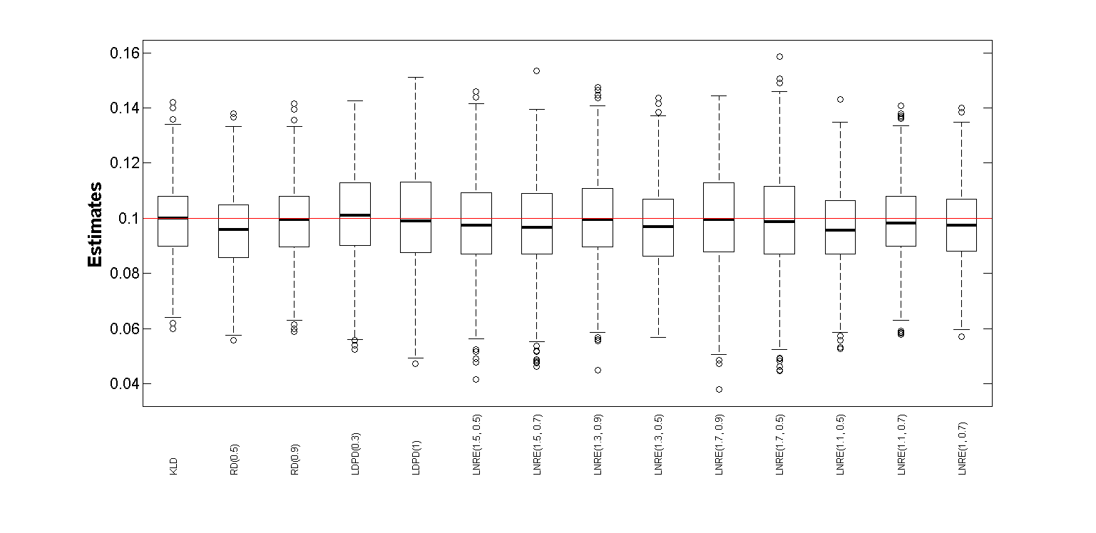

The LNRE measure and the associated minimum LNRE estimates are also used in constructing robust testing procedures for both one-sample and two sample hypothesis testing problems in [46, 47]. Their properties have also been investigated in detail which reveals similar advantages over the existing divergence based testing procedures, further indicating the usefulness of our new LNRE measures.
8 Conclusions
We believe that this paper has made several important contributions. We have proposed a new class of entropy measures and studied their properties in detail. This family has several distinguishing features, the most remarkable of which is the scale-invariance property. This two parameter family of entropies contains the Rényi entropy as a special case; the family can, in fact, be viewed as an appropriate Rényi entropy of the escort distribution associated with a given sub-probability distribution. We have derived the MaxEnt distribution corresponding to our family of entropies under the Tsallis non-extensive constraints. This is in fact the first scale-invariant family of generalized entropies which provides the usual Maxwell-Boltzmann MaxEnt theorem of Shannon under nonextensive conditions. The relation and link between this research and our previous work in [15] have also been carefully explained. And finally, we have developed the corresponding cross entropies and studied some of their important properties including those of their minimizers. We have also provided a sub-family of the cross entropy measures which leads to extensive results under the non-extensive framework, providing an instance of a case where the two concepts are combined.
The present paper further opens up several interesting future research problems. The first one would be the application of our new entropy and cross entropy measures in generalizing the concept of code-length or related information measures and the inference under source uncertainty or noisy channels. It will also be interesting to generalize and study the statistical physics and thermodynamic concepts through the use of the new LNE family and its MaxEnt distributions; this will generalize the Rényi thermodynamics and its applications. Since it is already known that the minimizer of the associated relative entropy measure leads to robust statistical inference [15], it will also be interesting to study the applications of the LNE, its MaxEnt and the LNCE measures in different statistical and general inferential problems which are expected to provide robust solutions under data contaminations or outliers. We hope to pursue some of these extensions in our future work.
Appendix A Important Definitions
Definition A.1 (-deformed functions)
For any , we define the -logarithm and -exponential of , respectively, as
| (58) | |||||
They coincide with the usual definitions of (natural) logarithm and exponential functions at .
Definition A.2 (-Escort Distribution)
Given a (sub-)probability distribution and , its escort probability distribution is defined as
| (62) |
Definition A.3 (The Correspondence)
Given a probability distribution , a function is said to be in correspondence with , denoted as , whenever they satisfy the relation (62).
Definition A.4 (-linear family)
For any fixed and given functions on a finite alphabet set , the corresponding -linear family of probability distributions on is defined as
| (63) |
When , the family is referred to as the linear family.
Definition A.5 (-power-law family)
Given any , a probability distribution (with full support when ), and , the -power-law family generated by and a set of given functions , , is defined as the set of probability distributions , , given by
| (64) | |||||
where is the normalizing constant. As , this distribution coincides with the classical exponential family of distribution given by
| (65) |
Definition A.6 (-mixture)
Given two probability distributions , any and , the -mixture of and is the probability distribution defined as
| (66) |
where is the required normalizing constant to make it into a probability distribution. It is important to note that for any non-trivial probability distribution , as noted in [28], and hence the above mixture distribution is well-defined.
Definition A.7 (-convex set)
A subset is called -convex for a given if for any and any their -mixture belongs to .
Definition A.8 (-concave functional)
A functional from to is said to be -concave for a given if for any and any their -mixture satisfies
| (67) |
The functional is said to be -convex if the inequality in (67) is reversed.
Definition A.9 (Algebraic inner Point)
Any probability distribution is called an algebraic inner point of the set if for any , there exists and such that .
Definition A.10 (Generalized Additivity Property of an Entropy)
An entropy functional, say , defined over , the set of sub-probability distributions in (3), is said to have the Generalized Additivity Property if there exists a strictly monotone and continuous function such that, for any and with , we have
| (68) |
where .
For the particular choice for some real , the relation (68) simplifies to
| (69) |
and it is referred to as the Additivity Property (or, Mean-Additivity property) of the entropy .
References
- [1] Abe, S. (2003). Geometry of escort distributions. Physical Review E, 68(3), 031101.
- [2] Aczel, J., and Daroczy Z. (1963). Characterisierung der entropien positiver ordnung und der Shannonschen entropie. Act. Math. Acad. Sci. Hunger., 14, 95–121.
- Basu et al. [1998] Basu, A., Harris, I.R., Hjort, N.L., and Jones, M.C. (1998). Robust and efficient estimation by minimising a density power divergence. Biometrika, 85, 549–559.
- [4] Basu, A., Shioya, H. and Park, C. (2011). Statistical Inference: The Minimum Distance Approach. Chapman & Hall/CRC. Boca Raton, Florida.
- [5] Beck, C., and Schogl, F. (1995). Thermodynamics of chaotic systems: an introduction (No. 4). Cambridge University Press.
- [6] Ben-Bassat, M., and Raviv, J. (1978). Rényi’s entropy and the probability of error. IEEE Transactions on Information Theory, 24(3), 324–331.
- [7] Boztas, S. (2014). On Rényi entropies and their applications to guessing attacks in cryptography. IEICE Transactions on Fundamentals of Electronics, Communications and Computer Sciences, 97(12), 2542–2548.
- [8] Bregman, L. M. (1967). The relaxation method of finding the common point of convex sets and its application to the solution of problems in convex programming. USSR computational mathematics and mathematical physics, 7(3), 200–217.
- [9] Bunte, C., and Lapidoth, A. (2014). Encoding tasks and Rényi entropy. IEEE Transactions on Information Theory, 60(9), 5065–5076.
- [10] Chapeau-Blondeau, F., Delahaies, A., and Rousseau, D. (2011). Source coding with Tsallis entropy. Electronics Letters, 47(3), 187–188.
- [11] Csiszár, I. (1991). Why least squares and maximum entropy? An axiomatic approach to inference for linear inverse problems. Annals of Statistics, 19(4), 2032–2066.
- [12] Dukkipati, A., Musti, N. M., and Bhatnagar, S. (2005). Properties of Kullback-Leibler cross entropy minimization in nonextensive framework. In: Information Theory, ISIT 2005. Proceedings. International Symposium on (pp. 2374-2378). IEEE.
- Fujisawa [2013] Fujisawa, H. (2013). Normalized estimating equation for robust parameter estimation. Electronic Journal of Statistics, 7, 1587–1606.
- [14] Gayen, A., and Kumar, M. A. (2019). Projection Theorems, Estimating Equations, and Power-Law Distributions. arXiv preprint, arXiv:1905.01434.
- [15] Ghosh, A., and Basu, A. (2018). A Generalized Relative ()-Entropy: Geometric Properties and Applications to Robust Statistical Inference. Entropy, 20(5), 347.
- [16] Hanawal, M. K., and Sundaresan, R. (2010). Guessing revisited: A large deviations approach. IEEE Transactions on Information Theory, 57(1), 70-78.
- [17] Hayashi, M., and Tan, V. Y. (2016). Equivocations, exponents, and second-order coding rates under various Rényi information measures. IEEE Transactions on Information Theory, 63(2), 975–1005.
- [18] Ho, S. W., and Verdu, S. (2015, June). Convexity/concavity of Rényi entropy and -mutual information. In: 2015 IEEE International Symposium on Information Theory (ISIT), (pp. 745-749). IEEE.
- [19] Jaynes, E. T. (1957a). Information Theory and Statistical Mechanics. Physical Review, Ser. II, 106 (4), 620–630.
- [20] Jaynes, E. T. (1957b). Information Theory and Statistical Mechanics II. Physical Review, Ser. II, 108 (2), 171–190.
- [21] Jizba, P., and Arimitsu, T. (2004). The world according to Rényi: thermodynamics of multifractal systems. Annals of Physics, 312(1), 17–59.
- [22] Jones, M. C., Hjort, N. L., Harris, I. R. and Basu A. (2001). A comparison of related density-based minimum divergence estimators. Biometrika, 88, 865–873.
- [23] Joshi, R., and Kumar, S. (2016). -Norm Information Measure and A Relation Between Coding and Questionnaire Theory. Open Systems and Information Dynamics, 23(03), 1650015.
- [24] Kapur, J.N. (1967). Generalized entropy of order and type . The Math. Seminar, 4, 78–82.
- [25] Kapur, J. N. (1969). Some properties of entropy of order and type . In: Proceedings of the Indian Academy of Sciences, Sec. A, 69(4), 201–211. Springer India.
- [26] Kapur, J. N. (1990). Maximum-Entropy Models in Science and Engineering. John Wiley, New York.
- [27] Kapur, J. N., and Kesavan, H. K. (1992). Entropy optimization principles and their applications. In: Entropy and energy dissipation in water resources, 3–20. Springer, Dordrecht.
- [28] Karthik, P. N., and Sundaresan, R. (2018). On The Equivalence of Projections in Relative -Entropy and Rényi Divergence. In: 2018 Twenty Fourth National Conference on Communications (NCC), 1–6. IEEE.
- [29] Kolmogorov, A. N. (1930). Sur la notion de la moyenne, Atti Accad. Naz. Lincei Mem. Cl. Sci. Fis. Mat. Natur. 12, 388–391.
- [30] Kosut, O., and Sankar, L. (2017). Asymptotics and non-asymptotics for universal fixed-to-variable source coding. IEEE Transactions on Information Theory, 63(6), 3757–3772.
- [31] Kullback, S. (1952). An application of information theory to multivariate analysis. Annals of Mathematical Statistics, 23(1), 88–102.
- [32] Kullback, S. (1953). A note on information theory. Journal of Applied Physics, 24(1), 106–107.
- [33] Kullback, S. (1954). Certain inequalities in information theory and the Cramer-Rao inequality. Annals of Mathematical Statistics, 25(4), 745–751.
- [34] Kullback, S. (1956). An application of information theory to multivariate analysis II. Annals of Mathematical Statistics, 27(1), 122–146. Correction p. 860.
- [35] Kullback, S. (1997). Information theory and statistics. Courier Corporation.
- [36] Kullback, S., and Leibler, R. A. (1951). On information and sufficiency. Annals of Mathematical Statistics, 22(1), 79–86.
- [37] Kumar, M. A., and Sason, I. (2016). Projection Theorems for the Rényi Divergence on -Convex Sets. IEEE Transactions on Information Theory, 62(9), 4924–4935.
- [38] Kumar, M. A., and Sason, I. (2016b). On projections of the Rényi divergence on generalized convex sets. In: 2016 IEEE International Symposium on Information Theory (ISIT) (pp. 1123–1127). IEEE.
- [39] Kumar, M. A., and Sundaresan, R. (2015a). Minimization Problems Based on Relative -Entropy I: Forward Projection. IEEE Transactions on Information Theory, 61(9), 5063–5080.
- [40] Kumar, M. A., and Sundaresan, R. (2015b). Minimization Problems Based on Relative -Entropy II: Reverse Projection. IEEE Transactions on Information Theory, 61(9), 5081–5095.
- [41] Kuzuoka, S. (2019). On the conditional smooth Rényi entropy and its applications in guessing and source coding. IEEE Transactions on Information Theory, 66(3), 1674–1690.
- [42] Lapidoth, A., and Pfister, C. (2019). Two measures of dependence. Entropy, 21(8), 778.
- [43] Lenzi, E. K., Mendes, R. S., and Da Silva, L. R. (2000). Statistical mechanics based on Rényi entropy. Physica A, 280(3-4), 337–345.
- [44] Liese, F., and Vajda, I. (1987). Convex statistical distances, Vol 95. Teubner.
- Lutwak et al. [2005] Lutwak, E., Yang, D., and Zhang, G. (2005). Cramear-Rao and moment-entropy inequalities for Rényi entropy and generalized Fisher information. IEEE Transactions on Information Theory, 51(2), 473–478.
- Maji et al. [2014] Maji, A., Ghosh, A. and Basu, A. (2014). The Logarithmic Super Divergence and its use in Statistical Inference. arXiv preprint, arXiv:1407.3961.
- Maji et al. [2016] Maji, A., Ghosh, A., and Basu, A. (2016). The Logarithmic Super Divergence and Asymptotic Inference Properties. AStA Advances in Statistical Analysis, 100(1), 99–131.
- [48] Nagumo, M. (1930). Uber eine Klasse der Mittelwerte. Japan. J. Math., 7, 71–79.
- [49] Nakiboglu, B. (2018). The Rényi capacity and center. IEEE Transactions on Information Theory, 65(2), 841–860.
- [50] Pardo, L. (2006). Statistical Inference based on Divergences. CRC/Chapman-Hall.
- [51] Rached, Z., Alajaji, F., and Campbell, L. L. (2001). Rényi’s divergence and entropy rates for finite alphabet Markov sources. IEEE Transactions on Information theory, 47(4), 1553–1561.
- [52] Rényi, A. (1961). On Measures of Entropy and Information. In: Proceedings of the Fourth Berkeley Symposium on Mathematical Statistics and Probability, Vol. 1. The Regents of the University of California.
- [53] Sason, I. (2015). On the Rényi divergence, joint range of relative entropies, and a channel coding theorem. IEEE Transactions on Information Theory, 62(1), 23–34.
- [54] Sason, I. (2018). Tight bounds on the Rényi entropy via majorization with applications to guessing and compression. Entropy, 20(12), 896.
- [55] Sason, I., and Verdu, S. (2017). Arimoto–Rényi conditional entropy and Bayesian -ary hypothesis testing. IEEE Transactions on Information theory, 64(1), 4–25.
- [56] Sason, I., and Verdu, S. (2018). Improved bounds on lossless source coding and guessing moments via Rényi measures. IEEE Transactions on Information Theory, 64(6), 4323–4346.
- [57] Shannon, C. E. (1948). A mathematical theory of communication. Bell System Tech. J., 27(3), 379–423.
- [58] Stummer, W., and Vajda, I. (2012). On Bregman distances and divergences of probability measures. IEEE Transactions on Information Theory, 58(3), 1277–1288.
- [59] Sundaresan, R. (2007). Guessing under source uncertainty. IEEE Transactions on Information Theory, 53(1), 269–287.
- [60] Tsallis, C. (1988). Possible generalization of Boltzmann-Gibbs statistics. Journal of statistical physics, 52(1-2), 479–487.
- [61] Tsallis, C. (2009). Introduction to nonextensive statistical mechanics : approaching a complex world. Springer, New York.
- [62] Tsallis, C., Mendes, R., and Plastino, A. R. (1998). The role of constraints within generalized nonextensive statistics. Physica A, 261(3-4), 534–554.
- [63] Vajda, I. (1989). Theory of statistical inference and information, Vol 11. Kluwer Academic Pub.
- [64] Van Erven, T., and Harremos, P. (2014). Rényi divergence and Kullback-Leibler divergence. IEEE Transactions on Information Theory, 60(7), 3797–3820.
- [65] Yu, L., and Tan, V. Y. (2018). Rényi resolvability and its applications to the wiretap channel. IEEE Transactions on Information Theory, 65(3), 1862–1897.
- [66] Yu, L., and Tan, V. Y. (2019). Simulation of random variables under Rényi divergence measures of all orders. IEEE Transactions on Information Theory, 65(6), 3349–3383.