Coupled fast and slow feedbacks lead to continual evolution: A general modeling approach

In order to focus our argument, we use a general model of an evolving trait for a single species, which can be extended to multiple species:

Here $u$ represents the population density distribution over the trait space. In the general case the evolving trait is not specified and therefore its trait space could be anything. The external factors (abiotic factors, species without evolving traits) are captured in $\varphi$. The function $f(u,\varphi)$ describes the growth of the population (which can depend on the distribution in trait space $u$ as well as the external factors $\varphi$). The function $g(u)$ describes the change in the trait due to mutations. The function $g$ does not incorporate how well these phenotypes perform (the change due to mutations is modeled in an unbiased manor), the change of the trait to more fit individuals comes from the modelling of the growth of all phenotypes. The function $h(u,\varphi)$ describes the change in external factors, which can depend on the phenotype densities $u$. Time scale differences between growth, external factors and mutations are captured in $\epsilon_{e}$ and $\epsilon_{m}$.

We include a possible polymorphic trait distribution (as is preferable argued by [16] and also used in [17]). A polymorphic trait distribution arises easily with asexual reproduction or traits that are determined by a few loci, but can also arise when assortive mating develops (see the discussion in [18]). We use an approach including genetic variation by modeling the populations with differential equations, which also releases the assumption that mutations have to cause an infinitesimal change in the trait value.

An example of a slow negative feedback is a predator prey interaction, where the generation time of the predator is much slower than that of the prey and the predator predates preferable on prey with a specific phenotype. An example of the specificity of the predator is predators preferring a certain size of prey (e.g. bears preferring large salmon [19] or zooplankton preferring phytoplankton with a certain nitrogen:phosphorus ratio [14]). Other examples besides predator-prey interactions include: a herbivore that changes the vegetation which then becomes less suitable for the herbivore; micro-organisms that produce a compound that inhibits them but is diluted in a large volume (to achieve the feedback being slow); a species with a complex life cycle with a habitat shift (with an evolvable component), if a crowded habitat has a delayed effect on the habitat quality; or a more complicated response of the whole ecosystem that leads to a negative feedback (e.g. with intransitive cycles as in [20]). The last example includes cases where the feedback is caused by human intervention, such as flu vaccinations—common viruses will be vaccinated against during the next season.

The fast positive feedback is an Allee effect on the phenotype. This could be due to for example finding mates (if the trait has effect on suitability of mates), cooperation in defense or in feeding. An example is when the adaptive trait is foraging on a certain vegetation type, the positive feedback could be that the more individuals forage in the same place, the better they are protected against predation. Or in the case of a habitat shift in the life cycle, similar habitat shift will share the second habitat with more individuals, providing mates or protection.

The best way to understand the system is to reduce it to the simplest version. Therefore we start with an simple version of a trait with only two possible phenotypes, one that is interacting with a external feedback and one that is not (or less strongly) (see Figure 1A). Although the main objective of this simplification is to understand the mechanisms that lead to continual evolution, this representation also reflects a biological system where a trait is either present or not at all, e.g. choosing one host or another. When the trait also affects mate choice (e.g. because they will be located near the same host), the trait has a positive feedback. The slow negative feedback results from the fact that one of the hosts can develop defenses.

We analyse the system where both phenotypes and the feedback change over time. We assume that the phenotypes have a positive feedback effect, i.e. the more individuals with a certain phenotype, the higher the growth rate of that phenotype. To be precise, we study the following system with the interacting phenotype $A$ (the phenotype choosing the host that can develop defenses), the (less) interacting phenotype $B$ (the phenotype choosing the host that cannot develop defenses) and the feedback compound $\varphi$ (the amount of defense in the host population that can develop defenses in the example):

The growth functions of the phenotypes $f_{A}$ and $f_{B}$ include the positive feedback. $\varphi$ is increased more by $A$ than by $B$ which is incorporated in the function $h$. Mutations are possible from one phenotype to the other with the mutation function $g$. $\epsilon_{m}$ and $\epsilon_{e}$ denote the different timescales of the population dynamics (no $\epsilon$), the feedback dynamics ($\epsilon_{e}$) and the evolutionary dynamics ($\epsilon_{m}$). We have modeled a positive effect of $A$ on $\varphi$ and a negative effect of $\varphi$ on $A$, but all our results are also valid for the opposite, then we can substitute $\varphi$ by $-\varphi$.

We prove that, for the system in Figure 1A and Equations (2) and with only slight restrictions on the functions $f$, $g$ and $h$, if we can choose $\epsilon_{e}$ and $\epsilon_{m}$ sufficiently small, the system will exhibit continual evolution for almost all initial states. The detailed proof is in the Supplementary Information section 4.1 and 4.2; the reasoning is as follows: First, we prove the case of a constant population size, where we can describe our system by the feedback compound $\varphi$ and the ratio $(R)$ between the two phenotypes. Observing that the proof for this case does not rely upon knowing the exact value of $\frac{dR}{dt}$ but merely the sign, we can extend the proof to systems where the population size is not fixed, by adopting an assumption controlling the sign of $\frac{dR}{dt}$. There are several possibilities but we used the ’unique stable value assumption’: when we keep $\varphi$ fixed and know $A$ there is only one value of $B$ that guarantees a stable state, and likewise when we know $B$ there is only one value of $A$. The proof only requires knowledge of the sign in a subregion of the domain.

The idea of the proof for a variable population size is illustrated in Figure 2B. The diagrams show an approximation of the dynamics in the ($A$,$B$) phase planes. This approximation is without the mutation term, but since mutations are rare (in our case the mutation term is small), the actual phase plane is very similar to the one shown. When at some point the feedback level is intermediate, there are 4 intersections of the lines $\frac{dA}{dt}=0$ and $\frac{dB}{dt}=0$ of which one is repelling (the origin), one is a saddle point (the point in the middle) and the other two are attracting (the nature of the equilibria can be seen from the sign of the derivatives). Depending on the initial densities of $A$ and $B$ the system goes to an attracting point near the $A$-axis or the $B$-axis. When this is near the $A$-axis, $B$ will be almost 0 and since $A$ is interacting strongly with the feedback compound, $\varphi$ will increase. This will in turn change the phase plane diagram and the intersection near the $A$-axis will become repelling. Then there is only one attracting intersection and that is near the $B$-axis and the system will approach that state. Since the dynamics in $\varphi$ are slower than in $A$ and $B$, the system will come close to the intersection near the $B$-axis before $\varphi$ changes significantly. When $\varphi$ changes we are back to the initial figure for intermediate $\varphi$, but now $\varphi$ will continue to decrease and the intersection near the $B$-axis will disappear. This will continue indefinitely and therefore will lead to continual evolution.

We only need some restrictions on the functions $f$, $g$ and $h$ and do not use any functional forms in our proof. Figure 2 illustrates the simulation of an example system. We show continual evolutionary cycles for 2 different initial states if $\epsilon_{e}$ and $\epsilon_{m}$ are chosen sufficiently small. With a high mutation rate and/or a fast feedback a stable equilibrium will be reached (leading to stasis), while lack of mutations causes one of the two phenotypes to go extinct.

For studying the case of a multi-valued trait, the evolving trait is represented as a range of values, and the external factor is represented by a scalar quantity (normalised between 0 and 1). We can then describe the system with the following set of differential equations:

We split the population in discrete groups $u_{i}$ with similar trait values. We show that the assumptions of a fast positive feedback and a slow negative feedback on the phenotype in this otherwise general model lead to continual evolution. These assumptions are given by restrictions on the functions $f$ and $h$. We can extend the reasoning from the previous section to a multi-valued trait. With a multi-valued trait we mean a trait with more than two phenotypes or an approximation of a continuous trait, such as length or level of toxin production. An overview of the system is shown in Figure 3A, where the trait values are scaled from 0 to 1 according to the strength of their negative feedback. We call these phenotypes $i$, and the density of individuals with phenotype $i$ is denoted by $u_{i}$. The feedback compound is again called $\varphi$ and can be the same quantities as in the previous section. For the positive feedback we use the population average of the trait, which we call $M$. We assume that when the level of $\varphi$ is so low that phenotypes with higher $i$ have higher growth rates for a certain phenotype distribution, growth rates will keep increasing with $i$ when we increase $M$ (and vice versa, if $\varphi$ is high and growth rates decrease with $i$, a decrease in $M$ will not change this). We use the assumption that the growth rate is either strictly increasing or strictly decreasing in the trait (therefore one of the extreme traits always has the highest fitness).

Analogous to the system with two phenotypes, we can prove the existence of evolutionary fluctuations under conditions mimicking our earlier assumptions. In the multiple phenotype setting there is one subtle point in the proof, where an additional assumption is needed to guarantee relatively quick changes in phenotypes. One possible additional assumption guaranteeing such rapid fluctuations is the existence of mutations from any trait value to any other trait value. In practical settings this assumptions will not always be applicable. For example, the assumption is more realistic when the trait value describes enzyme levels or levels of toxin production, than when considering length of a species, as we expect length to evolve gradually. An alternative assumption will be discussed later.

The proof that we can choose the timescales to obtain continual evolutionary dynamics is outlined in Fig. 3B, and described in detail in the Supplementary Information section 4.3. Here we provide an outline: We scale $\varphi$ also between 0 and 1 and without loss of generality may assume that $\varphi$ tends to $M$. Then, when for example $M$ is high and $\varphi$ is low, $\varphi$ will increase (blue arrows in Fig. 3B) because $\varphi$ goes to $M$. At some point $\varphi$ and $M$ will cross, in which case $M$ must already be declining and will continue to decline. The assumed fast positive feedback ensures that $M$ decreases drastically in a time interval in which $\varphi$ hardly changes, leading to symmetric conditions and hence continual evolutionary oscillations (green arrows in Fig. 3B).

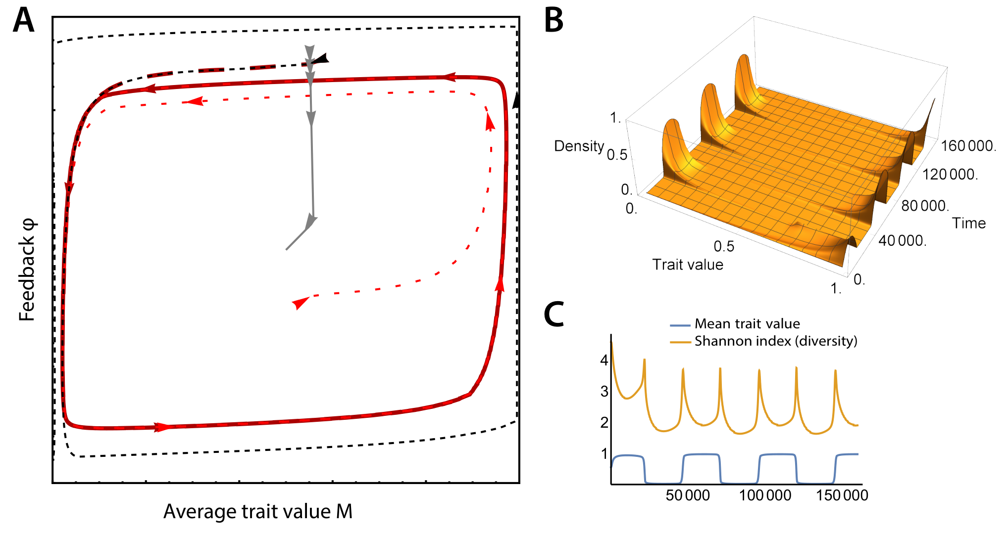
Again our proof is context free and applies to a wide variety of equations; an example is given in Figure 4. In Figure 4A demonstrates that turning off evolution leads to extinction of all but one phenotype, fast feedback leads to an equilibrium, and slow feedback leads to continual fluctuations. Figure 4B shows the distribution of phenotypes over time, and in 4C it is shown that the diversity of phenotypes increases at shifts of the mean trait value.

If we do not want to assume the existence of mutations from any phenotype to any other phenotype, we can adopt an alternative assumption, namely that the negative feedback is chosen sufficiently slow depending on the rate of mutations. In some circumstances this may even mean that the rate at which $\varphi$ changes is even slower than the mutation rate. This alternative assumption again may or may not be desirable in practice.

In natural systems, multiple traits determine the fitness in an individual. An extension of our model to more traits will give a more realistic picture of the dynamics we expect in natural populations. We extended the system to a species with two different traits that are both associated with a different negative feedback. The number of possible phenotypes is now the product of the number of phenotypes for each of the traits. In the most simple case, there are four phenotypes in the population: (1) high susceptibility for both feedbacks, (2) low susceptibility for both feedbacks, and (3 and 4) high susceptibility for one and low for the other (Figure 5A). Simulations with this extended system show that this system can also lead to continual adaptation and that the dynamics generally become irregular (Figure 5B). Looking at the change of the diversity index over time, we can conclude that there is no fixed period in the dynamics (Figure 5C). The example with multiple traits shows that we do not expect a natural system to come back to exactly the same state in a regular fashion.

In the previous section we assumed that $\frac{dR}{dt}$ depends only on $R$ and $\varphi$. When the total population size is not assumed to be fixed, such an assumption is not realistic. However, it turns out that the mechanism causing the drastic fluctuations can still occur without this assumption. The important observation is that to prove the existence of large fluctuations, we merely need to know the signs of $\frac{dR}{dt}$ and $\frac{d\varphi}{dt}$, and not the exact values.

Suppose now that we have two distinct traits, with population sizes $A$ and $B$. We do not assume that $A+B$ is constant, but will still write

Thus $R$ takes on values in the interval $[0,1]$. We assume that the total population will remain bounded, from above as well as below, so that $R\rightarrow 0$ corresponds to the extinction of population $A$, and $R\rightarrow 1$ to the extinction of population $B$. One naturally assumes that apart from mutations $dA/dt=0$ when $A=0$, and similarly $dB/dt=0$ when $B=0$, to obtain a system of differential equations of the form

As before, $\varphi$ will play the role of a strong negative feedback. We will assume that the functions $f_{A},f_{B},g,$ and $h$ are all continuously differentiable, and the constants $\epsilon_{m}$ and $\epsilon_{e}$ will be chosen arbitrarily small.

The existence of a positive ecological feedback on the populations $A$ and $B$ leads to the following assumption:

1. (PF)

   For all values of $A,B,$ and $\varphi$ we have

   $$\left(\frac{\partial}{\partial A}-\frac{\partial}{\partial B}\right)f_{A}>0,\;\;\mathrm{and}\;\;\left(\frac{\partial}{\partial B}-\frac{\partial}{\partial A}\right)f_{B}>0.$$

Thus, if an amount of $B$ is replaced by an equal amount of $A$ while $\varphi$ remains fixed, the fitness of the population $A$ increases while the fitness of the population $B$ decreases.

The next assumption, which we will refer to as the unique stable value assumption, will be used to draw conclusions about the sign of $\frac{dR}{dt}$ without knowing the exact values of $A$ and $B$. We do not claim that this assumption is necessary, but it turns out to be satisfied in many models and is convenient:

1. (USV1)

   For fixed values of $B$ and $\varphi$, there is a unique value $A_{0}\geq 0$ such that

   $$f_{A}(A,B,\varphi)>0$$

   for $0\leq A<A_{0}$, and

   $$f_{A}(A,B,\varphi)<0$$

   for $A>A_{0}$.

2. (USV2)

   For fixed values of $A$ and $\varphi$, there is a unique value $B_{0}\geq 0$ such that

   $$f_{B}(A,B,\varphi)>0$$

   for $B<B_{0}$, and

   $$f_{B}(A,B,\varphi)<0$$

   for $B>B_{0}$.

For $\varphi$ fixed we can therefore consider $A_{0}$ as a graph $\eta_{A}(B,\varphi)$, and similarly $B_{0}=\eta_{B}(A,\varphi)$. The positive feedback condition guarantees the following:

We assume the existence of a strong negative feedback:

1. (NF1)

   The difference $f_{A}-f_{B}$ decreases with $\varphi$, while

   $$\left(\frac{\partial}{\partial A}-\frac{\partial}{\partial B}\right)h>0.$$

2. (NF2)

   There exists $0<\varphi_{--}<\varphi_{++}<1$ such that

   $$f_{B}>f_{A}$$

   whenever $\varphi>\varphi_{++}$, while

   $$f_{A}>f_{B}$$

   whenever $\varphi<\varphi_{--}$.

Hence, for $\varphi$ sufficiently large and $\varphi$ sufficiently small the level sets $\{f_{A}=0\}$ and $\{f_{B}=0\}$ do not intersect. We may write $\varphi_{++}$ and $\varphi_{--}$ for the maximal resp. minimal value of $\varphi$ for which the level sets intersect. For our argument it will be necessary that both $\varphi_{++}$ and $\varphi_{--}$ can be reached, hence we make a “transitivity” assumption:

1. (Tr)

   The function $h$ is strictly positive when $\varphi\leq\varphi_{++}$, $B=0$ and $A=\eta_{A}(0,\varphi_{++})$. Similarly, the function $h$ is strictly negative when $\varphi\geq\varphi_{--}$, $A=0$ and $B=\eta_{B}(0,\varphi_{--})$.

Let us consider, for a fixed value of $\varphi$, joint solutions of the two equations

It is clear that, besides the origin, there always is a unique solution on each of the axes. For $A,B>0$ it follows from Lemma 4 that there either is no solution or a unique solution, depending on the value of $\varphi$. For $\varphi=\varphi_{++}$ the intersection point of $\{f_{A}=0\}$ and $\{f_{B}=0\}$ lies in the axis $\{A=0\}$, while for $\varphi=\varphi_{--}$ the intersection point lies in the axis $\{B=0\}$. See Figure 8 for a simple depiction of the level sets $\{f_{A}=0\}$ (in red) and $\{f_{B}=0\}$ (in blue).

Let us consider the ecological dynamics in the $(A,B)$-plane caused by the differential equations

for a fixed value of $\varphi$. When $\varphi\leq\varphi_{--}$ or $\varphi\geq\varphi_{++}$ there are three fixed points where

namely the origin and the two intersection points of the curves $\{f_{A}=0\}$ and $\{f_{B}=0\}$ with the respective axes $\{B=0\}$ and $\{A=0\}$. The origin is always repelling. One of the points on the axes is a saddle fixed point, with stable manifold equal to the axis. The third fixed point is attracting, and all orbits of initial values not lying on the axes converge to this attracting fixed point.

When $\varphi_{--}<\varphi<\varphi_{++}$ there are four fixed points. Again the origin is a repelling fixed point. There are again two fixed points on the axes, which are now both attracting. Finally, there is an intersection point of the curves $\{f_{A}=0\}$ and $\{f_{B}=0\}$, and assumption (i) implies that this is a hyperbolic saddle fixed point. Its stable manifold is the separatrix of the two attracting basins.

Let us now consider the effect of the mutations, represented by $\epsilon_{m}\cdot g(A,B)$, on the dynamics in the $(A,B)$-plane in the case $\varphi_{--}<\varphi<\varphi_{++}$. The behavior near each of the fixed points is stable under small $C^{1}$-perturbations, and the qualitative behavior of the system is robust. Hence, by choosing $\epsilon_{m}$ sufficiently small, there will still be a repelling fixed point at the origin, and a saddle point with separatrix near the intersection point of the curves $\{f_{A}=0\}$ and $\{f_{B}=0\}$. The rest of the quadrant is attracted to neighborhoods of the original attracting fixed points. These neighborhoods can be chosen arbitrarily small by choosing $\epsilon_{m}$ sufficiently small. Note that the addition of mutations causes the axes to be repelling, hence the attracting fixed point no longer lies on the axis but sufficiently nearby.

Finally let us consider the full three-dimensional dynamical system, taking into account that $\varphi$ is not fixed. We assume that for given $t_{0}$ we have $\varphi(t_{0})<\varphi_{++}$, and that $(A(t_{0}),B(t_{0}))$ lies in the small attracting region near the $A$-axis. For any $\delta>0$ we can, by taking $\epsilon_{e}$ and $\epsilon_{m}$ sufficiently small, assume that $A(t_{0})-\eta_{A}(0,\varphi_{++})>-\delta$ and $B<\delta$. It follows that $h(A(t_{0}),B(t_{0}),\varphi(t_{0}))$ is strictly positive. It follows that $\varphi$ will continue to grow while $\varphi<\varphi_{++}+\delta$ and while $(A(t),B(t))$ remains trapped in the small attracting neighborhood near the $A$-axis.

Let us consider the first time $t_{1}$ at which either $\varphi\geq\varphi_{++}+\delta$ or at which $(A,B)$ leaves the small attracting neighborhood. In either case it follows that the orbit $(A(t),B(t))$ is guaranteed to approach the small attracting neighborhood near the $B$-axis. If $\epsilon_{e}$ is sufficiently small the value of $\varphi$ can only decrease arbitrarily little while this happens. The conclusion is that we end up with a time $t_{2}>t_{1}$ when $\varphi(t_{1})>\varphi_{--}$ and $(A(t_{2}),B(t_{2}))$ lies in the attracting neighborhood near the $B$-axis. By the symmetry of our assumptions the process will repeat itself. We have proved the following.

Let us recall that in the first setting, where we considered two traits and a constant total population size, the argument used that the rate at which the ratio $R=\frac{A}{A+B}$ changes is determined only by $R$ and $\varphi$. When the assumption on the constant population size was dropped, this was no longer the case, but we saw that the main idea of the argument can still be used because in the appropriate regions in $(R,\varphi$)-coordinates the sign of $\frac{\partial R}{\partial t}$ is still known. One can easily imagine that, under appropriate assumptions, the same approach can be used when dealing with more than two phenotypes. The good choice of $R$, a projection from many variables onto $\mathbb{R}$, is of course essential to the argument.

Let us present a particular family of systems with finitely many trait values. We consider $n+1$ different strains $u_{i}$, where the index $i\in[0,1]$ is of the form $\frac{j}{n}$. As before, we will stipulate a fast positive feedback and a slow but dominating negative feedback caused by a variable $\varphi$. We will assume that $\varphi$ is produced more by strains $u_{i}$ for $i$ large, and for fixed values of $u=(u_{0},\ldots,u_{1})$ converges towards the average index $M$ given by

In the setting with multiple traits, knowledge of $M$ and $\varphi$ will not be sufficient to determine $dM/dt$ and $d\varphi/dt$. However, we will present assumptions where the signs of $dM/dt$ and $d\varphi/dt$ can be determined, at least in the relevant regions, which will be sufficient to guarantee large fluctuations.

Looking first only at the ecological factors of the dynamical system, ignoring the effects due to mutations, we assume that the densities of the individuals with phenotype $i$ change according to the equations

where the growth rates $\mu=(\mu_{0},\ldots,\mu_{1})$ are strictly positive, depend continuously on $u$ and $\varphi$, and for any given values of $u$ and $\varphi$ the tuple $(\mu_{0},\cdots,\mu_{1})$ is assumed to be either independent of $i$ or strictly monotonic in $i$. When $\mu$ is constant the relative population sizes do not change, and it follows that $\frac{dM}{dt}=0$.

We will assume that the rate of change of the feedback variable $\varphi$ can be written as

where the constant $\epsilon_{e}$ will later be assumed to be sufficiently small and $h$ is continuously differentiable. We make the following “negative feedback” assumption:

1. (NF1)

   The function $h$ satisfies $h<0$ when $\varphi>M$, and $h>0$ when $\varphi<M$.

An example of such a function is $h(u)=M(u)-\varphi$, but it is not necessarily the case that $h$ can be expressed as a function of $M$. The NF1 assumption of course implies that for each value of $M$ there is a unique value $\varphi=\varphi(M)$ for which $h=0$. The assumption that this unique value equals $M$ is merely a convenience, which by the Implicit Function Theorem can be obtained by a change of coordinates whenever $\frac{\partial h}{\partial\varphi}(u,\varphi)\neq 0$ is satisfied for all $u$ and $\varphi=\varphi(M)$.

We will make the following additional assumptions guaranteeing both a negative and a positive feedback.

1. (NF2)

   There exist $1>\varphi_{+}>\varphi_{-}>0$ with the following property: For any given non-zero $u$, the rates $\mu$ are decreasing in $i$ for $\varphi>\varphi_{+}$, and increasing in $i$ for $\varphi<\varphi_{-}$.

2. (PF)

   For each $\varphi$ there is a unique value $M_{\varphi}$ such that $\mu$ is strictly increasing at $(u,\varphi)$ whenever $M(u)>M_{\varphi}$, and strictly decreasing whenever $M(u)<M_{\varphi}$. We assume that $M_{\varphi}$ is non-decreasing with $\varphi$.

In other words, when $\mu$ is non-decreasing, it must remain so when $\varphi$ is decreased or when $M(u)$ is increased, and in the latter case must become strictly increasing. Similarly, when $\mu$ is non-increasing, it must remain so when $\varphi$ is increased or when $M(u)$ is decreased, in the latter case it must again become strictly decreasing.

By continuity of $\mu$ it follows from (PF) that $\mu$ is constant when $M(u)=M_{\varphi}$. Note that we may redefine $\varphi_{+}$ as the smallest $\varphi$ for which $M_{\varphi}=1$, and similarly $\varphi_{-}$ as the largest $\varphi$ for which $M_{\varphi}=0$. Note also that we do not assume that $\mu$ is a function of $M$.

Let us now add mutations to the model:

We assume that each function $g_{i}$ is non-negative when $u_{i}=0$, is decreasing in $u_{i}$, and is strictly increasing in each $u_{j}$ for $j\neq i$. In particular $g_{i}$ is strictly positive when $u_{i}=0$ but $u\neq 0$, thus mutations from any strain to any other strain are possible. We will later discuss alternative assumptions, making it possible to restrict some of the mutations.

If we drop the assumption that mutations from any strain to any other strain are possible, and replace it instead by the much weaker assumption that given any two strains $u_{i}$ and $u_{j}$ there is a possible sequence of mutations from $u_{i}$ to $u_{j}$, Lemma 7 fails, and the above proof breaks down. We cannot guarantee that at time $t_{2}$ the strain $u_{0}$ has increased to a definite size, independent of $\epsilon_{m}$, and as a result we cannot give a bound on the time interval $t_{3}-t_{2}$.

This issue can be solved by assuming that the constant $\epsilon_{e}$ is sufficiently small, where the bound on $\epsilon_{e}$ may have to depend on the choice of $\epsilon_{m}$. Note the difference with the above statement, which holds whenever both $\epsilon_{m}$ and $\epsilon_{e}$ are sufficiently small. In practice the stronger assumption on $\epsilon_{e}$, which can imply that $\epsilon_{e}$ is much smaller than $\epsilon_{m}$, may or may not be desirable.

The Shannon diversity index (H) is used in ecological research to describe species richness. Here we used the measure to describe phenotype richness within a species (we do not discuss whether bimodal phenotype distributions lead to different species). We calculate this diversity with the following formula:

Where $n$ is the number of phenotypes and $p_{i}$ the proportion of phenotype $i$ in the population.

In section 4.1 we give a proof for a system with two phenotypes and a fixed population size, and in this section we made an example of such a system. For this example we used the following equations:

$R$ and $\varphi$ are short for $R{t}$ and $\varphi{t}$ since they are time dependent. $R$ is the ratio of the two phenotypes, $A$ and $B$ ($r=\frac{A}{B})$, where $A$ is the phenotype interacting with the negative feedback $\varphi$. Figure 10 shows the result of time simulations of the example.

In section 4.2 we give a proof for a system with a variable population size. An example is shown in Figure 2 in the main text and the equations for the time derivatives of the populations with phenotypes $A$ and $B$ and the inhibitor $\varphi$ for that figure are:

References

- [1] Michael J Wiser, Noah Ribeck, and Richard E Lenski. Long-term dynamics of adaptation in asexual populations. Science, 342(6164):1364–1367, 2013.
- [2] Michael A Brockhurst, Tracey Chapman, Kayla C King, Judith E Mank, Steve Paterson, and Gregory DD Hurst. Running with the red queen: the role of biotic conflicts in evolution. Proceedings of the Royal Society of London B: Biological Sciences, 281(1797):20141382, 2014.
- [3] Leigh Van Valen. A new evolutionary law. Evolutionary theory, 1:1–30, 1973.
- [4] Nils Chr Stenseth and J Maynard Smith. Coevolution in ecosystems: Red queen evolution or stasis? Evolution, 38(4):870–880, 1984.
- [5] Geerat J Vermeij and Peter D Roopnarine. Reining in the red queen: the dynamics of adaptation and extinction reexamined. Paleobiology, 39(4):560–575, 2013.
- [6] Lee Hsiang Liow, Leigh Van Valen, and Nils Chr Stenseth. Red queen: from populations to taxa and communities. Trends in ecology & evolution, 26(7):349–358, 2011.
- [7] Kjetil L Voje, Øistein H Holen, Lee Hsiang Liow, and Nils Chr Stenseth. The role of biotic forces in driving macroevolution: beyond the red queen. Proc. R. Soc. B, 282(1808):20150186, 2015.
- [8] Jan Martin Nordbotten and Nils C Stenseth. Asymmetric ecological conditions favor red-queen type of continued evolution over stasis. Proceedings of the National Academy of Sciences, 113(7):1847–1852, 2016.
- [9] Ulf Dieckmann, Paul Marrow, and Richard Law. Evolutionary cycling in predator-prey interactions: population dynamics and the red queen. Journal of theoretical biology, 176(1):91–102, 1995.
- [10] Akihiko Mougi and Yoh Iwasa. Evolution towards oscillation or stability in a predator–prey system. Proceedings of the Royal Society of London B: Biological Sciences, page rspb20100691, 2010.
- [11] Paul Marrow, Richard Law, and C Cannings. The coevolution of predator—prey interactions: Esss and red queen dynamics. Proc. R. Soc. Lond. B, 250(1328):133–141, 1992.
- [12] Paul Marrow and Chris Cannings. Evolutionary instability in predator-prey systems. Journal of theoretical biology, 160(2):135–150, 1993.
- [13] Ulf Dieckmann and Richard Law. The dynamical theory of coevolution: a derivation from stochastic ecological processes. Journal of mathematical biology, 34(5-6):579–612, 1996.
- [14] Pedro Branco, Martijn Egas, James J Elser, and Jef Huisman. Eco-evolutionary dynamics of ecological stoichiometry in plankton communities. The American Naturalist, 192(1):E000–E000, 2018.
- [15] Peter A Abrams. The evolution of predator-prey interactions: theory and evidence. Annual Review of Ecology and Systematics, 31(1):79–105, 2000.
- [16] Richard Law, Paul Marrow, and Ulf Dieckmann. On evolution under asymmetric competition. Evolutionary Ecology, 11(4):485–501, 1997.
- [17] Jan D Van Der Laan and Pauline Hogeweg. Predator—prey coevolution: interactions across different timescales. Proc. R. Soc. Lond. B, 259(1354):35–42, 1995.
- [18] E Kisdi, FJA Jacobs, and SAH Geritz. Red queen evolution by cycles of evolutionary branching and extinction. Selection, 2(1-2):161–176, 2002.
- [19] SM Carlson, TP Quinn, and AP Hendry. Eco-evolutionary dynamics in pacific salmon. Heredity, 106(3):438, 2011.
- [20] Juan A Bonachela, Meike T Wortel, and Nils Chr Stenseth. Eco-evolutionary red queen dynamics regulate biodiversity in a metabolite-driven microbial system. Scientific reports, 7(1):17655, 2017.
- [21] F Dercole, R Ferriere, A Gragnani, and S Rinaldi. Coevolution of slow–fast populations: evolutionary sliding, evolutionary pseudo-equilibria and complex red queen dynamics. Proceedings of the Royal Society of London B: Biological Sciences, 273(1589):983–990, 2006.
- [22] Alexander I Khibnik and Alexey S Kondrashov. Three mechanisms of red queen dynamics. Proceedings of the Royal Society of London B: Biological Sciences, 264(1384):1049–1056, 1997.
- [23] Geerat J Vermeij. Unsuccessful predation and evolution. The American Naturalist, 120(6):701–720, 1982.
- [24] Takehito Yoshida, Laura E Jones, Stephen P Ellner, Gregor F Fussmann, and Nelson G Hairston Jr. Rapid evolution drives ecological dynamics in a predator–prey system. Nature, 424(6946):303, 2003.
- [25] Anton Crombach and Paulien Hogeweg. Chromosome rearrangements and the evolution of genome structuring and adaptability. Molecular biology and evolution, 24(5):1130–1139, 2007.
- [26] Anton Crombach and Paulien Hogeweg. Evolution of evolvability in gene regulatory networks. PLoS computational biology, 4(7):e1000112, 2008.
- [27] Benjamin H Good, Michael J McDonald, Jeffrey E Barrick, Richard E Lenski, and Michael M Desai. The dynamics of molecular evolution over 60,000 generations. Nature, 551(7678):45, 2017.
- [28] Meike T Wortel, Evert Bosdriesz, Bas Teusink, and Frank J Bruggeman. Evolutionary pressures on microbial metabolic strategies in the chemostat. Scientific reports, 6:29503, 2016.
- [29] Michael Doebeli and Iaroslav Ispolatov. Diversity and coevolutionary dynamics in high-dimensional phenotype spaces. The American Naturalist, 189(2):105–120, 2017.