Semi-supervised learning in unbalanced and heterogeneous networks

Imbalance is widely observed in real-world networks. For example, in gene interaction networks from the Saccharomyces Genome Database (SGD) [8], the number of viable genes can be four times that of inviable genes, which makes the dataset highly unbalanced. Networks in our analysis of real datasets analysis are also unbalanced according to the labels. When performing semi-supervised learning in network data, imbalance will cause significant bias if we do not take any action to rectify it. Labels (communities) with more members might be able to absorb more unlabeled nodes. Such bias should be dealt with in order to identify nodes in small communities. All of these problems are seldom discussed in the NSSL literature. In the present paper, we tackle the issue of network imbalance with our new algorithm by normalizing the weight of nodes.

A commonly used model for networks with community structures is the SBM, first presented by [13]. For decades, SBM has raised research interest in computer science, statistics, business studies as well as physics. Algorithms and consistency associated with community detection in SBM have been studied extensively. See, for example, [3, 29, 10, 12, 17, 20, 23]. However, due to the assumption of SBM, the nodes within the same community have the same degree ditribution, which is not observied in real-world datasets. Nodes in real networks often show degree heterogeneity even they have the same label (within the same community). Examples can be found in our real-data analysis. In order to accommodate hubs in networks, Karrer and Newman proposed the degree-corrected stochastic block model (DCBM) in [19]. The theoretical property of DCBM has been studied for community detection problem in [15, 20, 31, 11]. However, to the best of our knowledge, we are the first to apply the DCBM to the NSSL problem. In the present paper, we not only study the NSSL problem in homogeneous networks but also in heterogeneous ones. We propose the partially labeled DCBM (pDCBM) to model the generation of data and prove the consistency of our new algorithm.

We summarize the main results of this paper as follows:

We organize the rest of the paper as follows. We propose a new algorithm called WIL for the NSSL problem in Section 2, and explain it from the angles of information propagation, the regularization framework and first hitting time in random walks. In Section 3, we first propose a generative model, the partially labeled DCBM (pDCBM) to describe the NSSL problem. Statistical guarantee and phase boundary are also discussed in Section 3 under the pDCBM framework. In Section 4 and Section 5, we show the numerical results of our new method and cutting-edge methods using both simulation data and real-world networks. We review and summarize related work in Section 6. Finally, in Section 7, we conclude the paper and suggest directions for future work. The technical proof of main results is given in the Appendix.

We will first present the algorithm and then show some its explanations. We obtain $F$, the matrix of the class label scores, by applying the WIL algorithm: $F=(\rho W+(1-\rho)W^{T})Y,$ where $W=(I-\alpha\hat{D}^{-1}A)^{-1}$, and both $\alpha$ and $\rho$ are positive parameters less than 1. To understand WIL, we can write $W=\sum_{i=0}^{\infty}(\alpha\hat{D}^{-1}A)^{i},$ so that WIL combines the global link information with exponential decade random work and eliminates the effect of hubs by dividing $A$ by $\hat{D}.$ By performing global integration and normalizing degrees, WIL can overcome the issue of imbalance and heterogeneity in networks. The algorithm can be summarized as follows:

The formulation of WIL is motivated by the idea of information propagation. WIL is a combination of two different kinds of information propagation processes.

First, we consider $\hat{F}=\hat{W}Y=(I-\alpha\hat{D}^{-1}A)^{-1}Y$, which can also be written as an information propagation process:

Algorithm 2, which is also mentioned by [32], can be understood intuitively in terms of spreading label information with normalization on targeting points. We use adjacency matrix $A$ to spread the label, while we normalize rows of $A$ with degree of nodes. Figure 2 gives a toy example of one-step information propagation from node $i$’s neighbors to node $i$ in Algorithm 2.

$\tilde{F}=\hat{W}^{T}Y=(I-\alpha A\hat{D}^{-1})^{-1}Y$ can be written aster another information propagation algorithm:

The main difference in Algorithm 3 is that we normalize the label information by the degree of sourcing points. A toy example of one-step information propagation is given in Figure 3.

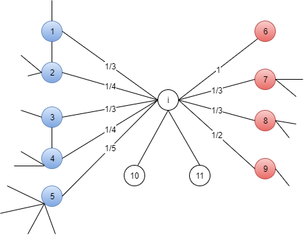
We raise examples for the above two different kinds of information propagation processes. For Algorithm 2, we take node $i$ as a student whose total social time is limited, so the influence from a certain friend would be averaged by the number of friends node $i$ has. In Algorithm 3, the social time of node $i$’s friends is also limited, so their influence should been normalized by their own degrees. Additionally, it is easy to show that bias introduced by imbalance is eliminated in some kind by the normalization in Algorithm 3. However, in the real world, it is not easy to tell exactly how does information propagate in the network. Therefore, we combine these two different kinds of information propagation in Algorithm 1 by introducing a weight parameter $\rho.$

Now, we develop regularization frameworks for the above two iteration algorithms. The cost function associated with $\hat{F}$ (Algorithm 2) is

here $\mu>0$ is a constant parameter. Set $\bar{F}=arg\min\limits_{F}Q_{1}(F).$ Then

Set $\alpha=\frac{1}{1+\mu},$ we have

which is the closed form of Algorithm 2.

Similarly, the cost function for $\tilde{F}$ (Algorithm 3) can be written as

here $\mu>0$ is a constant parameter. Set $\bar{F}=arg\min\limits_{F}Q_{2}(F).$ Then

Set $\alpha=\frac{1}{1+\mu},$ we have

which is the closed form of Algorithm 3.

Since we have assumed nodes with the same labels are more likely to be connected, a good classifying function should not change too much between linked points. The first term in both cost functions is the smoothness constraint. However, in $Q_{1}$ we simply calculate the $l_{2}$ norm between $F_{i}$ and $F_{j}$, while we normalize $F_{i}$ and $F_{j}$ by their respective degrees respectively in $Q_{2}$.

The second term is the fitting constraint, which means a good classifying function should not change too much from the initial label assignment. In $Q_{1}$, the fitting constraint can be written as $\sum_{i=1}^{n}\hat{d}_{i}\|F_{i}-Y_{i}\|^{2}.$ As for any node $j\in L$, predicting the $j^{\prime}s$ label wrongly will lead to $\hat{d}_{j}$ punishment. This is explained by Fig. 2 in which node $j$ with a larger degree gives more information that is wrong . However, in $Q_{2}$, the second term is $\sum_{i=1}^{n}\frac{1}{\hat{d}_{i}}\|F_{i}-Y_{i}\|^{2}$, which means the wrong information is normalized by the node’s degree. It can be understood from Fig 3 that the impact of one node on another is $\frac{1}{degree}.$

$\mu$ makes a trade-off between two competing constraints. Since $\alpha=\frac{1}{1+\mu}$, a large $\mu$ means more weight on the fitting constraint, which means a small $\alpha$ in both Algorithm 2 and Algorithm 3.

In the NSSL problem, it is essential to properly measure the closeness or similarity between every pair of nodes. One such possible measure is the first hitting time between nodes, if we cast the network into the context of random walks. This is partially motivated by the fact that random walks are easily trapped within nodes having the same labels.

Consider a random walk in a network: starting from a node, one of its edges is chosen with equal probability. Let $t_{i,j}$ denote the first hitting time from node $i$ to node $j$. Then $E(\exp(-\tau t_{i,j}))$ is a good local similarity measure between the two nodes, where the exponential transformation emphasizes the local information by down-weighting the long first hitting time. However, $E(\exp(-\tau t_{i,j}))$ is very difficult to calculate, so we approximate it by

It is easy to see that $H=(I-\alpha\hat{D}^{-1}A)^{-1}-I$. In this approximation, instead of counting only the first hitting time, we count all hitting times. Since $\exp(-\tau k)$ is very small when $k$ is large, the approximation is reasonable. In addition, we notice that $H$ is an asymmetric matrix and $h_{i,j}$ stands for the impact of node $j$ on node $i$. Finally, we add up $h_{i,j}$ and $h_{j,i}$ with weights $\rho$ and $1-\rho$ respectively to measure the similarity between nodes $i$ and $j$.

First, we introduce a prior distribution for the labels, a K-dimensional vector $\pi$ with $\sum_{i=1}^{K}\pi_{i}=1,$ to generate the labels. Let $B$ be the $K\times K$ symmetric probability matrix with $0\leq b_{i,j}\leq 1,\ \forall\ i,\ j\in\{1,2,\dots,K\}.$ Set membership vectors $z_{i}\in\{0,1\}^{K},$ where $z_{i,k}=1$ indicates that node $i$ belongs to label $k$. The DCBM introduces a set of degree-corrected parameters $\{\theta_{i}:i=1,\dots,n\}.$ As the given labels might be incorrect, we can also introduce the parameter $\nu\in[0,1]$ to represent the probability that the given labels are correct. Let $C$ be the $K\times K$ matrix where $C_{kk}=\nu$ for all $k,$ and $C_{kl}=\frac{1-\nu}{K-1}$ for $k\neq l.$ Let $A$ be the adjacency matrix of $G.$ We can define the generation process as follows:

• •

  Prior distribution of labels: $z_{i}\sim Mult(\cdot|\pi).$

• •

  For each node pair $(i,j)$, $A_{i,j}\sim Bern(\cdot|\theta_{i}\theta_{j}z_{i}Bz_{j}^{T}).$

• •

  For each labeled node, $y_{i}\sim Mult(\cdot|z_{i}C).$

Before presenting the main theories, we give useful notation first. For the pDCBM setting, we set $B=qE_{K}+(p-q)I_{K},$ where $E_{K}$ is a $K\times K$ matrix with elements all equal to $1$ and $p>q.$ We write $c(i)=k$ when the $i^{\prime}s$ label is $k$ and $\hat{c}(i)=k$ when the $i^{\prime}s$ predicted label is $k$ by applying the WIL algorithm with proper $\alpha$ and $\rho$. We set $n_{i}=|\{j|j\in G\and c(j)=i\}|$ and $l_{i}=|\{j|j\in L\and c(j)=i\}|.$ Let the known ratio $\delta=\frac{|L|}{|G|}.$ We consider the average error rate $err=\frac{1}{(1-\delta)n}\sum_{i\in U}1_{\hat{c}(i)\neq c(i)}$ and try to prove the weak consistency: for any $\epsilon>0$, $P(err\geq\epsilon)=f(n,\epsilon)\rightarrow 0.$

The main results of this paper are given as follows:

The technical proof of Theorem 4 is given in Appendix A.

The following theorem compares the phase boundaries for the unbalanced ratios of random walk (Algorithm 2), normalized Laplacian [32] (replacing $A\hat{D}^{-1}$ in Algorithm 3 by $\hat{D}^{-\frac{1}{2}}A\hat{D}^{-\frac{1}{2}}$) and Algorithm 3.

The following figure shows the boundaries of the three algorithms described in the above theorem.

Theorem 6 indicates that Algorithm 3 can tackle scenarios of greater imbalance than the other two methods, which is also observed in the empirical study.

Although Algorithm 3 gives sharper phase boundaries for unbalanced networks, in our simulation, Algorithm 2 has its own advantage when applied to balanced networks. We speculate that it is because Algorithm 2 does not rely on degree information as strongly as Algorithm 3 does, so the former might perform better in balanced networks and degree-corrected networks, where the degree information contains more noise than useful information. That is why we retain Algorithm 2 in WIL hoping we can learn the proper $\rho$ from the data itself. $\rho$ is supposed to be a trade-off for the importance of degree’s information.

Throughout the simulation studies, we use the pDCBM to generate networks with 2,000 nodes and two communities. We follow the simulation scheme in [3]. The community labels of nodes are outcomes of independent multinomial draws with $\pi=(\pi_{1},\pi_{2})$. Conditional on these labels, the edges are generated as independent Bernoulli variables with $p=B_{c(i),c(j)}$, while under the heterogeneous setting, $p=\theta_{i}\theta_{j}B_{c(i),c(j)}$. We use $\theta_{i}$ to represent the popularity of node $i$ and $\theta_{i}$’s are drawn independently with $P(\theta=0.2)=\gamma$ and $P(\theta=1)=1-\gamma$. We consider two settings, namely $\gamma=0$ and $\gamma=0.9$, which correspond to the homogeneous setting and the heterogeneous setting respectively.

The block probability matrix $B$ is determined by two parameters: the overall edge density $\lambda$ and the out-in ratio $\beta$. $\lambda$ is indeed $E(degree)$. It ranges from $2$ to $12$ in our simulations and a small $\lambda$ indicates a sparse network. $\beta$ determines the ratio of inter- to intra-community connection probabilities, and is set between $0.04$ and $0.4$. To generate $B$, we first generate $B^{(0)}$, whose diagonal and off-diagonal entries are set to $\beta^{-1}$ and $1$ respectively. Then $B^{(0)}$ is rescaled so that $E(degree)=\lambda$. Specifically,

$\rho$ selection: In following simulations and real-data analysis, we first select $\rho\in\mathcal{P}=\{0,0.1,0.2,\cdots,0.9,1\}$. By comparing the computing accuracy of labeled nodes, we select the $\rho$ with the best performance as the parameter to predict the unlabeled nodes in networks.

We repeat the random sampling code, and visualized the average choice of $\rho$ in different settings. In addition, we can also apply other optimization ideas to obtain a better $\rho$ but we will not discuss this in detail in this paper.

All of simulations below adopt the same network generation scheme as that described above. We control the parameters $\lambda$, $\beta$, $\gamma$ and $\pi$ to simulate different settings. Under each parameter setting, we replicate the simulation process 50 times (unless otherwise stated) and report the average performance of various methods.

We carry out extensive simulations to compare the WIL methods with the cutting-edge methods including algorithms introduced for graph-based semi-supervised learning (GSSL) in the literature. The following methods/algorithms are adopted for comparisons:

• •

  Partially absorbing random walks (PARW) [27],

• •

  Learning with local and global consistency (LGCiter) [32]

• •

  Semi-supervised learning using Gaussian fields and harmonic functions (HMNiter) [33]

• •

  Confidence-aware modulated label propagation (CAMLP) [28],

• •

  New regularized algorithms for transductive learning (MAD) [26]

References

- [1] Adamic, Lada A., and Natalie Glance. (2005). The political blogosphere and the 2004 US election: divided they blog. Proceedings of the 3rd international workshop on Link discovery. ACM, 2005.
- [2] A. L. Traud, P. J. Mucha, and M. A. Porter. Social structure of facebook networks. Physica A: Statistical Mechanics and its Applications, 391(16):4165–4180, 2012.
- [3] Amini, A. A., Chen, A., Bickel, P. J. and Levina, E. (2013). Pseudo-likelihood methods for community detection in large sparse networks. The Annals of Statistics. 41(4), 2097-2122.
- [4] Baluja, S., Seth, R., Sivakumar, D., Jing, Y., Yagnik, J., Kumar, S., … and Aly, M. (2008). Video suggestion and discovery for youtube: taking random walks through the view graph. In Proceedings of the 17th international conference on World Wide Web. (pp. 895-904). ACM.
- [5] Blum, A., and Chawla, S. (2001). Learning from labeled and unlabeled data using graph mincuts.
- [6] Cai, T. T., Liang, T., and Rakhlin, A. (2016). Inference via message passing on partially labeled stochastic block models. arXiv preprint arXiv:1603.06923.
- [7] Cai, T. T., Liang, T., and Rakhlin, A. (2017). Weighted Message Passing and Minimum Energy Flow for Heterogeneous Stochastic Block Models with Side Information. arXiv preprint arXiv:1709.03907.
- [8] Cherry, J. M., Adler, C., Ball, C., Chervitz, S. A., Dwight, S. S., Hester, E. T., … and Weng, S. (1998). SGD: Saccharomyces genome database. Nucleic acids research. 26(1), 73-79.
- [9] Du, C., and Zhao, Y. (2017). On Consistency of Graph-based Semi-supervised Learning. arXiv preprint arXiv:1703.06177.
- [10] Gao, C., Ma, Z., Zhang, A. Y., and Zhou, H. H. (2015). Achieving optimal misclassification proportion in stochastic block model. arXiv preprint arXiv:1505.03772.
- [11] Gao, C., Ma, Z., Zhang, A. Y., and Zhou, H. H. (2016). Community detection in degree-corrected block models. arXiv preprint arXiv:1607.06993.
- [12] Girvan, M. and Newman, M.E. (2002). Community structure in social and biological networks. Proceedings of the National Academy of Sciences. 99(12), 7821-7826.
- [13] Holland, P. W., Laskey, K. B., and Leinhardt, S. (1983). Stochastic blockmodels: First steps. Social networks. 5(2), 109-137.
- [14] JBlum, A., Lafferty, J., Rwebangira, M. R., and Reddy, R. (2004). Semi-supervised learning using randomized mincuts. In Proceedings of the twenty-first international conference on Machine learning. (p. 13). ACM.
- [15] Jin, J. (2015). Fast community detection by SCORE. The Annals of Statistics. 43(1), 57-89.
- [16] Joachims, T. (2003). ransductive learning via spectral graph partitioning. In Proceedings of the 20th International Conference on Machine Learning. (ICML-03) (pp. 290-297).
- [17] Joseph, A., and Yu, B. (2016). Impact of regularization on spectral clustering. The Annals of Statistics, 44(4), 1765-1791.
- [18] Kanade, V., Mossel, E., and Schramm, T. (2016). Global and local information in clustering labeled block models.IEEE Transactions on Information Theory. 62(10), 5906-5917.
- [19] Karrer, B. and Newman, M. E. (2011). Stochastic blockmodels and community structure in networks. Physical Review E. 83(1), 016107.
- [20] Lei, J. and Rinaldo, A. (2015). Consistency of spectral clustering in stochastic block models. The Annals of Statistics. 43(1), 215-237.
- [21] Orbach, M., and Crammer, K. (2012). Graph-based transduction with confidence. In Joint European Conference on Machine Learning and Knowledge Discovery in Databases. (pp. 323-338). Springer, Berlin, Heidelberg.
- [22] Peel, L. (2017). Graph-based semi-supervised learning for relational networks. In Proceedings of the 2017 SIAM International Conference on Data Mining. (pp. 435-443). Society for Industrial and Applied Mathematics.
- [23] Rohe, K., Chatterjee, S., and Yu, B. (2011). Spectral clustering and the high-dimensional stochastic blockmodel. The Annals of Statistics. 1878-1915.
- [24] Saade, A., Krzakala, F., Lelarge, M., and Zdeborová, L. (2016). Fast randomized semi-supervised clustering. arXiv preprint arXiv:1605.06422.
- [25] Subramanya, A., and Talukdar, P. P. (2014). Graph-based semi-supervised learning. Synthesis Lectures on Artificial Intelligence and Machine Learning. 8(4), 1-125.
- [26] Talukdar, P. P., and Crammer, K. (2009). New regularized algorithms for transductive learning. In Joint European Conference on Machine Learning and Knowledge Discovery in Databases. (pp. 442-457). Springer, Berlin, Heidelberg.
- [27] Wu, X. M., Li, Z., So, A. M., Wright, J., and Chang, S. F. (2012). Learning with partially absorbing random walks. In Advances in Neural Information Processing Systems (pp. 3077-3085).
- [28] Yamaguchi, Y., Faloutsos, C., and Kitagawa, H. (2016, May). CAMLP: Confidence-Aware Modulated Label Propagation. In SIAM International Conference on Data Mining.
- [29] Zhang A Y, Zhou H H. (2016). Minimax rates of community detection in stochastic block models. The Annals of Statistics. 44(5): 2252-2280.
- [30] Zhang, P., Moore, C., and Zdeborová, L. (2014). Phase transitions in semisupervised clustering of sparse networks. Physical Review E. 90(5), 052802.
- [31] Zhao, Y., Levina, E., and Zhu, J. (2012). Consistency of community detection in networks under degree-corrected stochastic block models. The Annals of Statistics. 40(4), 2266-2292.
- [32] Zhou, D., Bousquet, O., Lal, T. N., Weston, J., and Schölkopf, B. (2004). Learning with local and global consistency. In Advances in neural information processing systems. (pp. 321-328).
- [33] Zhu, X., Ghahramani, Z., and Lafferty, J. D. (2003). Semi-supervised learning using gaussian fields and harmonic functions. In Proceedings of the 20th International conference on Machine learning. (ICML-03) (pp. 912-919).