Composite optimization for robust blind deconvolutionThanks: Department of Mathematics, U. Washington, Seattle, WA 98195; www.math.washington.edu/ddrusv. Research of Drusvyatskiy was supported by the NSF DMS 1651851 and CCF 1740551 awards.
Abstract
The blind deconvolution problem seeks to recover a pair of vectors from a set of rank one bilinear measurements. We consider a natural nonsmooth formulation of the problem and show that under standard statistical assumptions, its moduli of weak convexity, sharpness, and Lipschitz continuity are all dimension independent. This phenomenon persists even when up to half of the measurements are corrupted by noise. Consequently, standard algorithms, such as the subgradient and prox-linear methods, converge at a rapid dimension-independent rate when initialized within constant relative error of the solution. We then complete the paper with a new initialization strategy, complementing the local search algorithms. The initialization procedure is both provably efficient and robust to outlying measurements. Numerical experiments, on both simulated and real data, illustrate the developed theory and methods.
1 Introduction
A variety of tasks in data science amount to solving a nonlinear system , where is a highly structured smooth map. The setting when is a quadratic map already subsumes important problems such as phase retrieval [47, 12, 37], blind deconvolution [4, 33, 36, 49], matrix completion [13, 18, 48], and covariance matrix estimation [15, 35], to name a few. Recent works have suggested a number of two-stage procedures for globally solving such problems. The first stage—initialization—yields a rough estimate of an optimal solution, often using spectral techniques. The second stage—local refinement—uses a local search algorithm that rapidly converges to an optimal solution, when initialized at . For a detailed discussion, we refer the reader to the recent survey [16].
The typical starting point for local refinement is to form an optimization problem
| (1.1) |
where is a carefully chosen penalty function and is a constraint set. Most widely-used penalties are smooth and convex; e.g., the squared -norm is ubiquitous in this context. Equipped with such penalties, the problem (1.1) is smooth and therefore gradient-based methods become immediately applicable. The main analytic challenge is that the condition number of the problem (1.1) often grows with the dimension of the ambient space . This is the case for example for phase retrieval, blind deconvolution, and matrix completion problems; see e.g. [16] and references therein. Consequently, generic nonlinear programming guarantees yield efficiency estimates that are far too pessimistic. Instead, a fruitful strategy is to recognize that the Hessian may be well-conditioned along the “relevant” set of directions, which suffice to guarantee rapid convergence. This is where new insight and analytic techniques for each particular problem come to bare (e.g. [49, 37, 39]).
Smoothness of the penalty function in (1.1) is crucially used by the aforemention techniques. A different recent line of work [25, 20, 21, 6] has instead suggested the use of nonsmooth convex penalties—most notably the -norm . Such a nonsmooth formulation will play a central role in our work. A number of algorithms are available for nonsmooth compositional problems (1.1), most notably the subgradient method
and the prox-linear algorithm
The local convergence guarantees of both methods can be succinctly described as follows. Set and suppose there exist constants satisfying:
- •
(approximation) for all ,
- •
(sharpness) for all ,
- •
(Lipschitz bound) for all with .
Then when equipped with an appropriate sequence and initialized at a point satisfying , both the subgradient and prox-linear iterates will converge to an optimal solution of the problem. The prox-linear algorithm converges quadratically, while the subgradient method converges at a linear rate governed by the ratio .
A possible advantage of nonsmooth techniques can be gleaned from the phase retrieval problem. The papers [25, Corollary 3.1,3.2], [21, Corollary 3.8] recently, showed that for the phase retrieval problem, standard statistical assumptions imply that with high probability all the constants are dimension independent. Consequently, completely generic guarantees outlined above, without any modification, imply that both methods converge at a dimension-independent rate, when initialized within constant relative error of the optimal solution. This is in sharp contrast to the smooth formulation of the problem, where a more nuanced analysis is required, based on restricted smoothness and convexity. Moreover, this approach is robust to outliers in the sense that analogous guarantees persist even when up to half of the measurements are corrupted by noise.
In light of the success of the nonsmooth penalty approach for phase retrieval, it is intriguing to determine if nonsmooth techniques can be fruitful for a wider class of large-scale problems. Our current work fits squarely within this research program. In this work, we analyze a nonsmooth penalty technique for the problem of blind deconvolution. Formally, we consider the task of robustly recovering a pair from bilinear measurements:
| (1.2) |
where is an arbitrary noise corruption with frequency that is at most one half, and and are known measurement vectors. Such bilinear systems and their complex analogues arise often in biological systems, control theory, coding theory, and image deblurring, among others. Most notably such problems appear when recovering a pair from the convolution measurements When passing to the Fourier domain this problem is equivalent to that of solving a complex bilinear system of equations; see the pioneering work [4]. All the arguments we present can be extended to the complex case. We focus on the real case for simplicity.
In this work we analyze the following nonsmooth formulation of the problem:
| (1.3) |
where is a user-specified constant and . Our contributions are two-fold:
- 1.
(Local refinement) Suppose that the vectors and are both i.i.d. Sub-Gaussian and satisfy a mild growth condition (which is automatically satisfied for Gaussian random vectors). We will show that as long as the number of measurements satisfies , the formulation (1.3) admits dimension independent constants , , and with high probability. Consequently, subgradient and prox-linear methods rapidly converge to the optimal solution at a dimension-independent rate when initialized at a point with constant relative error . Analogous results also hold under more general incoherence assumptions.
- 2.
(Initialization) Suppose now that and are both i.i.d. Gaussian and are independent from the noise . We develop an initialization procedure that in the regime and , will find a point satisfying , with high probability. To the best of our knowledge, this is the only available initialization procedure with provable guarantees in presence of gross outliers. We also develop complementary guarantees under the weaker assumption that the vectors corresponding to exact measurements are independent from the noise in the outlying measurements. This noise model allows one to plant outlying measurements from a completely different pair of signals, and is therefore computationally more challenging.
The literature studying bilinear systems is rich. From the information-theoretic perspective [34, 17, 29], the optimal sample complexity in the noiseless regime is if no further assumptions (e.g. sparsity) are imposed on the signals. Therefore, from a sample complexity viewpoint, our guarantees are optimal. Incidentally, to our best knowledge, all alternative approaches are either suboptimal by a polylogarithmic factor in or require knowing the sign pattern of one of the underlying signals [3, 4].
Recent algorithmic advances for blind deconvolution can be classified into two main approaches: works based on convex relaxations and those employing gradient descent on a smooth nonconvex function. The influential convex techniques of [3, 4] “lift” the objective to a higher dimension, thereby necessitating the resolution of a high-dimensional semidefinite program. The more recent work of [1, 2] instead relaxes the feasible region in the natural parameter space, under the assumption that the coordinate signs of either or are known a priori. Finally, with the exception of [4], the aforementioned works do not provide guarantees in the noisy regime.
Nonconvex approaches for blind deconvolution typically apply gradient descent to a smooth formulation of the problem [33, 37, 27]. Since the condition number of the problem scales with dimension, as we mentioned previously, these works introduce a nuanced analysis that is specific to the gradient method. The authors of [33] propose applying gradient descent on a regularized objective function, and identify a “basin of attraction” around the solution. The paper [37] instead analyzes gradient descent on the unregularized objective. They use the leave-one-out technique and prove that the iterates remain within a region where the objective function satisfies restricted strong convexity and smoothness conditions. The sample complexities of the methods in [33, 37, 27, 37] are optimal up to polylog factors.
The nonconvex strategies mentioned above all use spectral methods for initialization. These methods are not robust to outliers, since they rely on the leading singular vectors/values of a potentially noisy measurement operator. Adapting the spectral initialization of [25] to bilinear inverse problems enables us to deal with gross outliers of arbitrary magnitude. Indeed, high variance noise makes it easier for our initialization to “reject” outlying measurements.
The outline of the paper is as follows. Section 2 records basic notation we will use throughout the paper. Section 3 reviews the impact of sharpness and weak convexity on the rapid convergence of numerical methods. Section 4 establishes estimates of weak convexity, sharpness, and Lipschitz moduli for the blind deconvolution problem under both deterministic and statistical assumptions on the data. Section 5 introduces the initialization procedure and proves its correctness even if a constant fraction of measurements is corrupted by gross outliers. The final Section 6 presents numerical experiments illustrating the theoretical results in the paper.
2 Notation
The section records basic notation that we will use throughout the paper. To this end, we always endow with the dot product, , and the induced norm . The symbol denotes the unit sphere in , while denotes the open unit ball. When convenient, we will use the notation to emphasize the dimension of the ambient space. More generally, will stand for the open ball around of radius . We define the distance and the nearest-point projection of a point onto a closed set by
respectively. For any pair of real-valued functions , the notation means that there exists a positive constant such that for all . We write if both and
We will always use the trace inner product on the space of matrices . The symbols and will denote the operator and Frobenius norm of , respectively. Assuming , the map returns the vector of ordered singular values . Note the equalities and .
Nonsmooth functions will appear throughout this work. Consequently will use some basic constructions of generalized differentiation, as set out for example in the monographs [45, 38, 8, 42]. Consider a function and a point , with finite. Then the Fréchet subdifferential of at , denoted by , is the set of all vectors satisfying
| (2.1) |
Thus, a vector lies in the subdifferential precisely when the function locally minorizes up to first-order. We say that a point is stationary for whenever the inclusion, , holds. Standard results show for convex functions the subdifferential reduces to the subdifferential in the sense of convex analysis, while for differentiable functions it consists only of the gradient .
Notice that in general, the little-o term in (2.1) may depend on the base-point , and the estimate (2.1) therefore may be nonuniform. In this work, we will only encounter functions whose subgradients automatically satisfy a uniform type of lower-approximation property. We say that a function is -weakly convex11 1 Weakly convex functions also go by other names such as lower-, uniformly prox-regularity, paraconvex, and semiconvex. if the perturbed function is convex. It is straightforward to see that for any -weakly convex function , subgradients automatically satisfy the uniform bound:
We will comment further on the class of weakly convex functions in Section 3.
We say a that a random vector in is -sub-gaussian whenever for all vectors . The sub-gaussian norm of a real-valued random variable is defined to be , while the sub-exponential norm is defined by . Given a sample we will write to denote its median.
3 Algorithms for sharp weakly convex problems
The central thrust of this work is that under reasonable statistical assumptions, the penalty formulation (1.3) satisfies two key properties: (1) the objective function is weakly convex and (2) grows at least linearly as one moves away from the solution set. In this section, we review the consequences of these two properties for local rapid convergence of numerical methods. The discussion mostly follows the recent work [20], though elements of this viewpoint can already be seen in the two papers [25, 21] on robust phase retrieval.
Setting the stage, we introduce the following assumption.
Assumption A.
Consider the optimization problem,
| (3.1) |
Suppose that the following properties hold for some real .
- 1.
(Weak convexity) The set is closed and convex, while the function is -weakly convex.
- 2.
(Sharpness) The set of minimizers is nonempty and the inequality
The class of weakly convex functions is broad and its importance in optimization is well documented [44, 43, 40, 46, 5]. It trivially includes all convex functions and all -smooth functions with Lipschitz gradient. More broadly, it includes all compositions
where is convex and -Lipschitz, and is -smooth with -Lipschitz Jacobian. Indeed then the composite function is weakly convex with parameter ; see e.g. [24, Lemma 4.2]. In particular, our target problem (1.3) is clearly weakly convex, being a composition of the norm and a quadratic map. The estimate on the weak convexity constant is often much too pessimistic, however. Indeed, under statistical assumptions, we will see that the target problem (1.3) has a much better weak convexity constant. The notion of sharpness, and the related error bound property, is now ubiquitous in nonlinear optimization. Indeed, sharpness underlies much of perturbation theory and rapid convergence guarantees of various numerical methods. For a systematic treatment of error bounds and their applications, we refer the reader to the monographs of Dontchev-Rockafellar [22] and Ioffe [28], and the article of Lewis-Pang [31].
Taken together, weak convexity and sharpness provide an appealing framework for deriving local rapid convergence guarantees for numerical methods. In this work, we specifically focus on two such procedures: the subgradient and prox-linear algorithms. To this end, we aim to estimate both the radius of rapid converge around the solution set and the rate of convergence. Our ultimate goal is to show that when specialized to our target problem (1.3), with high probability, both of these quantities are independent of the ambient dimensions and as soon as the number of measurements is sufficiently large.
Both the subgradient and prox-linear algorithms have the property that when initialized at a stationary point of the problem, they could stay there for all subsequent iterations. Since we are interested in finding global minima, and not just stationary points, we must therefore estimate the neighborhood of the solution set that has no extraneous stationary points. This is the content of the following simple lemma [20, Lemma 3.1].
Lemma 3.1.
Proof.
Fix a critical point . Letting , we deduce . Dividing by , the result follows. ∎
The estimate of the radius in Lemma 3.1 is tight. To see this, consider minimizing the univariate function on the real line . Observe that the set of minimizers is , while is always an extraneous stationary point. A quick computation shows that the smallest valid weak convexity is while the largest valid sharpness constant is .
We therefore deduce . Hence the radius of the region that is devoid of extraneous stationary points is tight.
In light of Lemma 3.1, let us define for any the tube
| (3.2) |
Thus we would like to search for algorithms whose basin of attraction is a tube for some numerical constant . Due to the above discussion, such a basin of attraction is in essence optimal.
We next discuss two rapidly converging algorithms. The first is the Polyak subgradient method, outlined in Algorithm 1. Notice that the only parameter that is needed to implement the procedure is the minimal value of the problem (3.1). This value is sometimes known; case in point, the minimal value of the penalty formulation (1.3) is zero when the bilinear measurements are exact.
Choose . If , then exit algorithm.
Set .
The rate of convergence of the method relies on the Lipschitz constant and the condition measure:
A straightforward argument [20, Lemma 3.2] shows . The following theorem appears as [20, Theorem 4.1], while its application to phase retrieval was investigated in [21].
Theorem 3.2 (Polyak subgradient method).
When the minimal value of the problem (3.1) is unknown, there is a straightforward modification of the subgradient method that converges R-linearly. The idea is to choose a geometrically decaying control sequence for the stepsize. The disadvantage is that the convergence guarantees rely on being able to tune estimates of , , and .
Choose . If , then exit algorithm.
Update iterate .
The following theorem appears as [20, Theorem 6.1]. The convex version of the result dates back to Goffin [26].
Theorem 3.3 (Geometrically decaying subgradient method).
Notice that both subgradient algorithms 1 and 2 are at best locally linearly convergent, with a relatively cheap per-iteration cost. As the last example we discuss an algorithm that is specifically designed for convex compositions, which is locally quadratically convergent. The caveat is that the method may have a high per-iteration cost, since in each iteration one must solve an auxiliary convex optimization problem.
Setting the stage, let us introduce the following assumption.
Assumption B.
Consider the optimization problem,
| (3.5) |
Suppose that the following properties holds for some real .
- 1.
(Convexity and smoothness) The function and the set are convex and is differentiable.
- 2.
(Approximation accuracy) The convex models satisfy the estimate:
- 3.
(Sharpness) The set of minimizers is nonempty and the inequality
It is straightforward to see that Assumption B implies that is -weakly convex; see e.g. [24, Lemma 7.3]. Therefore Assumption B implies Assumption A.
Algorithm 3 describes the prox-linear method—a close variant of Gauss-Newton. For a historical account of the prox-linear method, see e.g., [10, 32, 24] and the references therein.
Set
The following theorem proves that under Assumption B, the prox-linear method converges quadratically, when initialized sufficiently close to the solution set. Guarantees of this type have appeared, for example, in [25, 23, 11, 23]. For the sake of completeness, we provide a quick argument.
Theorem 3.4 (Prox-linear algorithm).
4 Assumptions and Models
In this section, we aim to interpret the efficiency of the subgradient and prox-linear algorithms discussed in Section 3, when applied to our target problem (1.3). To this end, we must estimate the three parameters . These quantities control both the size of the attraction neighborhood around the optimal solution set and the rate of convergence within the neighborhood. In particular, we will show that these quantities are independent of the ambient dimension under natural assumptions on the data generating mechanism.
It will be convenient for the time being to abstract away from the formulation (1.3), and instead consider the function
where is an arbitrary linear map and is an arbitrary vector. The formulation (1.3) corresponds to the particular linear map . Since we will be interested in the prox-linear method, let us define the convex model
Our strategy is as follows. Section 4.1 identifies deterministic assumptions on the data, and , that yield favorable estimates of . Then Section 4.2 shows that these deterministic assumptions hold with high probability under natural statistical assumptions on the data generating mechanism.
4.1 Favorable Deterministic Properties
The following property, widely used in the literature, will play a central role in our analysis.
Assumption C (Restricted Isometry Property (RIP)).
There exist constants such that for all matrices of rank at most two the following bound holds:
The following proposition estimates the two constants and , governing the performance of the subgradient and prox-linear methods under Assumption C.
Proposition 4.1 (Approximation accuracy and Lipschitz continuity).
Suppose Assumption C holds and let be arbitrary. Then the following estimates hold:
Proof.
To see the first estimate, observe
where the last estimate follows from Young’s inequality Now suppose and . We then successively compute:
The proof is complete. ∎
We next move on to estimates of the sharpness constant . To this end, consider two vectors and , and set . Without loss of generality, henceforth, we suppose . Our estimates on the sharpness constant will be valid only on bounded sets. Consequently, define the two sets:
The set simply encodes a bounded region, while encodes all rank-1 factorizations of the matrix with bounded factors. We begin with the following proposition, which analyzes the sharpness properties of the idealized function
The proof is quite long, and therefore we have placed it in Appendix A.1.
Proposition 4.2.
For any , we have the following bound
Thus the function is sharp on the set with coefficient . We note in passing that the analogue of Proposition 4.2 for symmetric matrices was proved in [49, Lemma 5.4].
The sharpness of the loss in the noiseless regime (i.e. when ) is now immediate.
Proposition 4.3 (Sharpness in the Noiseless Regime).
Suppose that Assumption C holds and that equality, , holds. Then for any , we have the following bound:
Sharpness in the noisy case requires an additional assumption. We record it below. Henceforth, for any set , we define the restricted linear map by setting .
Assumption D (-outliner bounds).
There exists a set , vectors , , and a constant such that the following hold.
-
Equality holds for all .
-
For all matrices of rank at most two, we have
(4.1)
Combining Assumption D with Proposition 4.2 quickly yields sharpness of the objective even in the noisy setting.
Proposition 4.4 (Sharpness in the noisy regime).
Suppose that Assumption D holds. Then
Proof.
To summarize, suppose Assumptions C and D are valid. Then in the notation of Section 3 we may set:
Consequently, the tube radius of is and the the linear convergence rate of the subgradient method is governed by . In particular, the local search algorithms must be initialized at a point , whose relative distance to the solution set is upper bounded by a constant. We record this conclusion below.
4.2 Assumptions under generative models
In this section, we present natural generative models under which Assumptions C and D are guaranteed to hold. Recall that at the high level, we aim to recover the pair of signals based on given corrupted bilinear measurements . Formally, let us fix two disjoint sets and , called the inlier and outlier sets. Intuitively, the index set encodes exact measurements while encodes measurements that have been replaced by gross outliers. Define the corruption frequency ; henceforth, we will suppose Then for an arbitrary, potentially random sequence , we consider the measurement model:
| (4.2) |
In accordance with the previous section, we define the linear map by . To simplify notation, we let denote the matrix whose rows, in column form, are and we let denote the matrix whose rows are . Note that we make no assumptions about the nature of . In particular, can even encode exact measurements for a different signal.
We focus on two measurement matrix models. The first model requires both matrices and to be random. For simplicity, the reader may assume both are Gaussian with i.i.d. entries, though the results of this paper extend beyond this case. The second model allows semi-deterministic matrices, namely deterministic and Gaussian with i.i.d. entries. In the later parts of the paper, we will put further incoherence assumptions on the deterministic matrix .
Random matrix models.
- M1
The vectors and are i.i.d. realizations of -sub-gaussian random vectors and , respectively. Suppose moreover that and are independent and satisfy the nondegeneracy condition,
(4.3) for some real .
- M2
The matrix is arbitrary and the matrix is standard Gaussian.
Some comments are in order. The model M1 is fully stochastic, in the sense that and are generated by independent sub-gaussian random vectors. The nondegeneracy condition (4.3) essentially asserts that with positive probability, the products are non-negligible, uniformly over all unit norm rank two matrices . In particular, the following example shows that Gaussian matrices with i.i.d. entries are admissible under Model M1. In contrast, the model M2 is semi-stochastic: it allows to be deterministic, while making the stronger assumption that is Gaussian.
Example 4.1 (Gaussian Matrices Satisfy Model M1).
Assume that and are standard Gaussian random vectors in and , respectively. We claim this setting is admissible under M1. To see this, fix a rank 2 matrix having unit Frobenius norm. Consider now a singular value decomposition , and note the equality, . For each index define and . Then clearly are i.i.d. standard Gaussian; see e.g. [51, Exercise 3.3.6]. Thus, for any , we compute
Notice that conditioned on , we have . Thus letting be a standard normal, we have
Therefore, we may simply set and .
4.2.1 Assumptions C and D under Model M1
In this section, we aim to prove the following theorem, which shows validity of Assumptions C and D under M1, with high probability.
Theorem 4.6 (Measurement Model M1).
Consider a set satisfying . Then there exist constants depending only on such that the following holds. As long as , then with probability at least , every matrix of rank at most two satisfies
| (4.4) |
and
| (4.5) |
Due to scale invariance, in the proof we only concern ourselves with matrices of rank at most two satisfying . Let us fix such a matrix and an arbitrary index set with . We begin with the following lemma.
Lemma 4.7 (Pointwise concentration).
The random variable is sub-exponential with parameter . Consequently, the estimate holds:
| (4.6) |
Moreover, there exists a numerical constant such that for any , we have with probability at least the estimate:
| (4.7) |
Proof.
Markov’s inequality along with (4.3) implies
which is the lower bound in (4.6). Now we address the upper bound. To that end, suppose that has a singular value decomposition . We then deduce
where the second inequality follows since is a norm and [51, Lemma 2.7.7]. This bound has two consequences: first is a sub-exponential random variable with parameter and second see [51, Exercise 2.7.2]. The first bound will be useful momentarily, while the second completes the proof of (4.6).
Next define the sub-exponential random variable
Standard results (e.g. [51, Exercise 2.7.10]) imply for all . Using Bernstein inequality for sub-exponential random variables, Theorem C.6, to upper bound completes the proof. ∎
Proof of Theorem 4.6.
Choose and let be the ()-net guaranteed by Lemma C.2. Let denote the event that the following two estimates hold for all matrices in :
| (4.8) | ||||
| (4.9) |
Throughout the proof, we will assume that the event holds. We will estimate the probability of at the end of the proof. Meanwhile, seeking to establish RIP, define the quantity
We aim first to provide a high probability bound on .
Let be arbitrary and let be the closest point to in . Then we have
| (4.10) | ||||
| (4.11) |
where (4.10) follows from (4.7) and (4.11) follows from the triangle inequality. To simplify the third term in (4.11), using SVD, we deduce that there exist two orthogonal matrices of rank at most two satisfying With this decomposition in hand, we compute
| (4.12) |
where the second inequality follows from the definition of and the estimate Thus, we arrive at the bound
| (4.13) |
As was arbitrary, we may take the supremum of both sides of the inequality, yielding . Rearranging yields the bound
Assuming that , we further deduce that
| (4.14) |
establishing that the random variable is bounded by in the event .
Now let denote either or . We now provide a uniform lower bound on . Indeed,
| (4.15) | ||||
| (4.16) | ||||
| (4.17) | ||||
| (4.18) |
where (4.15) uses the forward and reverse triangle inequalities, (4.16) follows from (4.8), the estimate (4.17) follows from the forward and reverse triangle inequalities, and (4.18) follows from (4.12) and (4.14). Switching the roles of and in the above sequence of inequalities, and choosing , we deduce
In particular, setting , we deduce
and therefore using (4.6), we conclude the RIP property
| (4.19) |
Next, let and note that
Therefore every satisfies
| (4.20) |
Setting in (4.19) and (4.20), we deduce the claimed estimates (4.4) and (4.5). Finally, let us estimate the probability of . Using Lemma 4.7 and the union bound yields
where the second inequality follows from C.2 and is a constant.
Then we deduce since .
Hence as long as , we can be sure . The result follows immediately.
∎
Corollary 4.8 (Convergence guarantees).
Thus with high probability, if one initializes the subgradient and prox-linear methods at a pair satisfying , then the methods will converge to the optimal solution set at a dimension independent rate.
4.2.2 Assumptions C and D under Model M2
In this section, we verify Assumptions C and D under Model M2 and an extra incoherence condition. Namely, we impose further conditions on singular values of ()
which intuitively guarantee that the entries of any vector in are “well-spread.”
Proposition 4.9 (Measurement Model M2).
Assume Model M2 and fix an arbitrary index . Define the parameter
and suppose . Then there exist numerical constants such that with probability
every matrix of rank at most two satisfies
| (4.22) |
and
| (4.23) |
Proof.
The argument mirrors the proof of Proposition 4.6 and therefore we only provide a sketch. Fix a unit Frobenius norm matrix of rank at most two. We aim to show that for any fixed , the following random variable is highly concentrated around its mean:
To that end, fix a singular value decomposition . We then compute
where and are orthogonal, , and are i.i.d. standard normal random variables. This decomposition, together with the rotation invariance of the normal distribution, furnishes us with the following distributional equivalence:
where is a standard normal random variable. Consequently, we have the following expression for the expectation:
We now upper/lower bound this expectation. The upper bound follows from the estimate
The lower bound uses the following two dimensional inequality , which holds for all :
In particular, setting , we deduce
| (4.24) |
To establish concentration of the random variable , we apply a standard result (Theorem C.5) on the concentration of weighted sums of mean zero independent sub-gaussian random variables. In particular, to apply Theorem C.5, we write , and define weights
Noticing that , where is an absolute constant, and
it follows that for any fixed unit Frobenius norm matrix of rank at most two, with probability at least , we have
| (4.25) |
We have thus established concentration for any fixed . We now proceed with a covering argument in the same way as in the proof of Theorem 4.6. To this end, choose and let be the ()-net guaranteed by C.2. Let denote the event that the following two estimates hold for all matrices :
Throughout the proof, we will assume that the event holds. By exactly the same covering argument as in Theorem 4.6, setting with , we deduce
where either or .
5 Initialization
Previous sections have focused on local convergence guarantees under various statistical assumptions. In particular, under Assumptions C and D, one must initialize the local search procedures at a point , whose relative distance to the solution set is upper bounded by a constant. In this section, we present a new spectral initialization routine (Algorithm 4) that is able to efficiently find such point . The algorithm is inspired by [25, Section 4] and [52].
Before describing the intuition behind the procedure, let us formally introduce our assumptions. Throughout this section, we make the following assumption on the data generating mechanism, which is stronger than Model M1:
-
The entries of matrices and are i.i.d. Gaussian.
Our arguments rely heavily on properties of the Gaussian distribution. We note, however, that our experimental results suggest that Algorithm 4 provides high-quality initializations under weaker distributional assumptions.
Recall that in the previous sections, the noise was arbitrary. In this section, however, we must assume more about the nature of the noise. We will consider two different settings.
- N1
The measurement vectors and the noise sequence are independent.
- N2
The inlying measurement vectors and the corrupted observations are independent.
The noise models N1 and N2 differ in how an adversary may choose to corrupt the measurements. Model N1 allows an adversary to corrupt the signal, but does not allow observation of the measurement vectors . On the other hand, Model N2 allows an adversary to observe the outlying measurement vectors and arbitrarily corrupt those measurements. For example, the adversary may replace the outlying measurements with those taken from a completely different signal: for
Form directional estimates:
We can now describe the intuition underlying Algorithm 4. Throughout we denote unit vectors parallel to and by and , respectively. Algorithm 4 exploits the expected near orthogonality of the random vectors and to the directions and , respectively, in order to select a “good” set of measurement vectors. Namely, since , we expect minimal eigenvectors of and to be near and , respectively. Since our measurements are bilinear, we cannot necessarily select vectors for which and are both small, rather, we may only select vectors for which the product is small, leading to subtle ambiguities not present in [25, Section 4] and [52]; see Figure 1. Corruptions add further ambiguities since the noise model N2 allows a constant fraction of measurements to be adversarially modified.
Formally, Algorithm 4 estimates an initial signal in two stages: first it constructs a pair of directions which estimate the true directions
(up to sign); then it constructs an estimate of the signed signal norm , which corrects for sign errors in the first stage. We now discuss both stages in more detail, starting with the direction estimate. Most proofs will be deferred to Appendix B. The general proof strategy we follow is analogous to [25, Section 4] for phase retrieval, with some subtle modifications due to asymmetry.
Direction Estimate.
In the first stage of the algorithm, we estimate the directions and , up to sign. Key to our argument is the following decomposition for model N1 (which will be proved in Appendix B.1):
where and the matrices have small operator norm (decreasing with ), with high probability. Using the Davis-Kahan theorem [19], we can then show that the minimal eigenvectors of and are sufficiently close to and , respectively.
Proposition 5.1 (Directional estimates).
There exist numerical constants , so that for any and , with probability at least , the following hold:
Norm estimate.
In the second stage of the algorithm, we estimate as well as correct the sign of the direction estimates from the previous stage. In particular, for any define the quantity
| (5.1) |
where and are as in Theorem 4.6. Then we prove the following estimate (see Appendix B.2).
Proposition 5.2 (Norm Estimate).
Thus, the preceding proposition shows that tighter estimates on the norm result from better directional estimates in the first stage of Algorithm 4. In light of Proposition 5.2, we next estimate the probability of the event , which in particular implies with high probability .
Proposition 5.3 (Sign estimate).
Under either Model N1 and N2, there exist numerical constants such that if and , then the estimate holds:22 2 In the case of model N1, one can set .
Proof.
Using Theorem 4.6 and Propositions 5.1, we deduce that for any , with probability we have
Thus under model N1 it suffices to set . Then the probability of the event is at least . On the other hand, under model N2, it suffices to assume and then we can set . The probability of the event is then at least . Finally using the bound yields the result. ∎
Step 3: Final estimate.
Putting the directional and norm estimates together, we arrive at the following theorem.
Theorem 5.4.
There exist numerical constants such that if and , then for all , with probability at least we have
Proof.
Combining Corollary 4.5 and Theorem 5.4, we arrive at the following guarantee for the stage procedure.
Corollary 5.5 (Efficiency estimates).
Suppose either of the models N1 and N2. Let be the output of the initialization Algorithm 4. Set and consider the optimization problem
| (5.2) |
Set and notice that the feasible region of (5.2) coincides with . Then there exist constants and such that as long as and , the following properties hold with probability .33 3 In the case of model N1, one can set .
- 1.
- 2.
(prox-linear) Algorithm 3 initialized at (with appropriate ) converges quadratically:
Proof.
We provide the proof under model N1. The proof under model N2 is completely analogous. Combining Proposition 5.2, Proposition 5.3, and Theorem 5.4, we deduce that there exist constants such that as long as and , then for any , with probability , we have
| (5.3) |
and
In particular, notice from (5.3) that and therefore the feasible region contains an optimal solution of the original problem (1.3). Using Proposition 4.2, we have
Combining the estimates, we conclude
Thus to ensure the relative error assumption (4.21), it suffices to ensure the inequality
where are the constants from Corollary 4.8. Using the bound , it suffices to set
Thus the probability of the desired event becomes for some constant . Finally, using the bound and applying Corollary 4.8 completes the proof. ∎
6 Numerical Experiments
In this section we demonstrate the performance and stability of the prox-linear and subgradient methods, and the initialization procedure, when applied to real and artificial instances of Problem (1.3). All experiments were performed using the Julia [7] programming language.
Subgradient method implementation.
Implementation of the subgradient method for Problem (1.3) is simple, and has low per-iteration cost. Indeed, one may simply choose the subgradient
where denotes the sign of , with the convention The cost of computing this subgradient is on the order of four matrix multiplications. When applying Algorithm 2, choosing the correct parameters is important, since its convergence is especially sensitive to the value of the step-size decay ; the experiment described in Section 6.1.2, which aided us empirically in choosing for the rest of the experiments, demonstrates this phenomenon. Setting seemed to suffice for all the experiments depicted hereafter.
Prox-linear method implementation.
Recall that the convex models used by the prox-linear method take the form:
| (6.1) |
Equivalently, one may rewrite this expression as a Least Absolute Deviation (LAD) objective:
Thus, each iteration of Algorithm 3 requires solving a strongly convex optimization problem:
Motivated by the work of [25] on robust phase retrieval, we solve this subproblem with the graph splitting variant of the Alternating Direction Method of Multipliers, as described in [41]. This iterative method applies to problems of the form
Yielding the following subproblems, which are repeatedly executed:
where and are dual multipliers and is a control parameter. Each above step may be computed analytically. We found in our experiments that choosing and yielded fast convergence. Our stopping criteria for this subproblem is considered met when the primal residual satisfies and the dual residual satisfies with .
6.1 Artificial Data
We first illustrate the performance of the prox-linear and subgradient methods under noise model N1 with i.i.d. standard Gaussian noise . Both methods are initialized with Algorithm 4. We experimented with Gaussian noise of varying variances, and observed that higher levels did not adversely affect the performance of our algorithm. This is not surprising, since the theory suggests that both the objective and the initialization procedure are robust to gross outliers. We analyze the performance with problem dimensions and and with number of measurements with varying from to . In Fig. 2 and 3, we have depicted how the quantity
changes per iteration for the prox-linear and subgradient methods. We conducted tests in both the moderate corruption () and high corruption () regimes. For both methods, under moderate corruption () we see that exact recovery is possible as long as . Likewise, even in high corruption regime () exact recovery is still possible as long as . We also illustrate the performance of Algorithm 1 when there is no corruption at all in Fig. 2, which converges an order of magnitude faster than Algorithm 2.
In terms of algorithm performance, we see that the prox-linear method takes few outer iterations, approximately 15, to achieve very high accuracy, while the subgradient method requires a few hundred iterations. This behavior is expected as the prox-linear method converges quadratically and the subgradient method converges linearly. Although the number of iterations of the prox-linear method is small, we demonstrate in the sequel that its total run-time, including the cost of solving subproblems, can be higher than the subgradient method.
6.1.1 Number of matrix-vector multiplications
Each iteration of the prox-linear method requires the numerical resolution of a convex optimization problem. We solve this subproblem using the graph splitting ADMM algorithm, as described in [41], the cost of which is dominated by the number of matrix vector products required to reach the target accuracy. The number of “inner iterations” of the prox-linear method and thus the number of matrix vector products is not determined a priori. The cost of each iteration of the subgradient method, on the other hand, is on the order of 4 matrix vector products. In the subsequent plots, we solve a sequence of synthetic problems for and keep track of the total number of matrix-vector multiplications performed. We run both methods until we obtain . Additionally, we keep track of the same statistics for the subgradient method. We present the results in Fig. 4. We observe that the number of matrix-vector multiplications required by the prox-linear method can be much greater than those required by the subgradient method. Additionally, they seem to be much more sensitive to the ratio .
6.1.2 Choice of step size decay
Due to the sensitivity of Algorithm 2 to the step size decay , we experiment with different choices of in order to find an empirical range of values which yield acceptable performance. To that end, we generate synthetic problems of dimension and choose , and record the average error of the final iterate after iterations of the subgradient method for different choices of . The average is taken over test runs with . We test both noisy and noiseless instances to see if corruption of entries significantly changes the effective range of . Results are shown in Fig. 5.
6.1.3 Robustness to noise
We now empirically validate the robustness of the prox-linear and subgradients algorithms to noise. In a setup familiar from other recent works [25, 4], we generate phase transition plots, where the -axis varies with the level of corruption , the -axis varies as the ratio changes, and the shade of each pixel represents the percentage of problem instances solved successfully. For every configuration , we run experiments.
Noise model N1 - independent noise
Initially, we experiment with Gaussian random matrices and , the results for which can be found in Fig. 9.
The phase transition plots are similar for both dimensionality choices, revealing that in the moderate independent noise regime (), setting suffices. On the other hand, for exact recovery in high noise regimes (), one may need to choose as large as .
We repeat the same experiment in the setting where the matrix is deterministic and has orthogonal columns of Euclidean norm , and is a gaussian random matrix. Specifically, we take to be a partial Hadamard matrix, from the first columns of an Hadamard matrix. In that case, the operator can be computed efficiently in time by -padding to length and computing its Fast Walsh-Hadamard Transform (FWHT). Additionally, the products can also be computed in time by taking the FWHT of and keeping the first coordinates of the result.
Noise model N2 - arbitrary noise
We now repeat the previous experiments, but switch to noise model N2. In particular, we now adversarially hide a different signal in a subset of measurements, i.e., we set
where in the above is an arbitrary pair of signals. Intuitively, this is a more challenging noise model than N1, since it allows an adversary try to trick the algorithm into recovering an entirely different signal. Our experiments confirm that this regime is indeed more difficult for the proposed algorithms, which is why we only depict the range in Figs. 9 and 9 below.
6.2 Performance of initialization on real data
We now demonstrate the proposed initialization strategy on real world images. Specifically, we set and to be two random digits from the training subset of the MNIST dataset [30]. In this experiment, the measurement matrices have i.i.d. Gaussian entries, and the noise follows Model N1 with . We apply the initialization method and plot the resulting images (initial estimates) in Fig. 10. Evidently, the initial estimates of the images are visually similar to the true digits, up to sign; in other examples, the foreground appears to be switched with the background, which corresponds to the natural sign ambiguity. Finally, we plot the normalized error for the two recovery methods (subgradient and prox-linear) in Fig. 11.


6.3 Experiments on Big Data
We apply the subgradient method for recovering large-scale real color images . In this setting, so using Algorithm 1 is applicable with . We “flatten” the matrices into dimensional vectors . In contrast to the previous experiments, our sensing matrices are of the following form:
where is the symmetric normalized Hadamard matrix and is a diagonal random sign matrix. The same holds for . Notice that we can perform the operations in time: we first form the elementwise product between the signal and the random signs, and then take its Hadamard transform, which can be performed in flops. We can efficiently compute , required for the subgradient method, in a similar fashion. We recover each channel separately, which means we essentially have to solve three similar minimization problems. Notice that this results in dimensionality for each channel.
We observed that our initialization procedure (Algorithm 4) is extremely accurate in this setting. Therefore to better illustrate the performance of the local search algorithms, we perform the following heuristic initialization. For each channel, we first sample , rescale by the true magnitude of the signal, and run Algorithm 1 for one step to obtain our initial estimates .
An example where we recover a pair of color images using the Polyak subgradient method (Algorithm 1) is shown below; Fig. 12 shows the progression of the estimates , up until the -th iteration, while Fig. 13 depicts the normalized error at each iteration for the different channels of the images.


References
- [1] Alireza Aghasi, Ali Ahmed, and Paul Hand. Branchhull: Convex bilinear inversion from the entrywise product of signals with known signs. arXiv preprint arXiv:1702.04342, 2017.
- [2] Alireza Aghasi, Ali Ahmed, Paul Hand, and Babhru Joshi. A convex program for bilinear inversion of sparse vectors. arXiv preprint arXiv:1809.08359, 2018.
- [3] Ali Ahmed, Alireza Aghasi, and Paul Hand. Blind deconvolutional phase retrieval via convex programming. arXiv preprint arXiv:1806.08091, 2018.
- [4] Ali Ahmed, Benjamin Recht, and Justin Romberg. Blind deconvolution using convex programming. IEEE Transactions on Information Theory, 60(3):1711–1732, 2014.
- [5] Paolo Albano and Piermarco Cannarsa. Singularities of semiconcave functions in Banach spaces. In Stochastic analysis, control, optimization and applications, Systems Control Found. Appl., pages 171–190. Birkhäuser Boston, Boston, MA, 1999.
- [6] Yu Bai, Qijia Jiang, and Ju Sun. Subgradient descent learns orthogonal dictionaries. arXiv preprint arXiv:1810.10702, 2018.
- [7] Jeff Bezanson, Alan Edelman, Stefan Karpinski, and Viral B Shah. Julia: A fresh approach to numerical computing. SIAM review, 59(1):65–98, 2017.
- [8] J.M. Borwein and Q.J. Zhu. Techniques of Variational Analysis. Springer Verlag, New York, 2005.
- [9] Stéphane Boucheron, Gábor Lugosi, and Pascal Massart. Concentration inequalities: A nonasymptotic theory of independence. Oxford university press, 2013.
- [10] J.V. Burke. Descent methods for composite nondifferentiable optimization problems. Math. Programming, 33(3):260–279, 1985.
- [11] J.V. Burke and M.C. Ferris. A Gauss-Newton method for convex composite optimization. Math. Programming, 71(2, Ser. A):179–194, 1995.
- [12] E.J. Candès, X. Li, and M. Soltanolkotabi. Phase retrieval via Wirtinger flow: theory and algorithms. IEEE Trans. Inform. Theory, 61(4):1985–2007, 2015.
- [13] E.J. Candès and B. Recht. Exact matrix completion via convex optimization. Found. Comput. Math., 9(6):717–772, 2009.
- [14] Emmanuel J Candes and Yaniv Plan. Tight oracle inequalities for low-rank matrix recovery from a minimal number of noisy random measurements. IEEE Transactions on Information Theory, 57(4):2342–2359, 2011.
- [15] Yuxin Chen, Yuejie Chi, and Andrea J. Goldsmith. Exact and stable covariance estimation from quadratic sampling via convex programming. IEEE Trans. Inform. Theory, 61(7):4034–4059, 2015.
- [16] Yuejie Chi, Yue M Lu, and Yuxin Chen. Nonconvex optimization meets low-rank matrix factorization: An overview. arXiv preprint arXiv:1809.09573, 2018.
- [17] Sunav Choudhary and Urbashi Mitra. Sparse blind deconvolution: What cannot be done. In Information Theory (ISIT), 2014 IEEE International Symposium on, pages 3002–3006. IEEE, 2014.
- [18] Mark A Davenport and Justin Romberg. An overview of low-rank matrix recovery from incomplete observations. arXiv preprint arXiv:1601.06422, 2016.
- [19] Chandler Davis and William Morton Kahan. The rotation of eigenvectors by a perturbation. iii. SIAM Journal on Numerical Analysis, 7(1):1–46, 1970.
- [20] Damek Davis, Dmitriy Drusvyatskiy, Kellie J MacPhee, and Courtney Paquette. Subgradient methods for sharp weakly convex functions. arXiv preprint arXiv:1803.02461, 2018.
- [21] Damek Davis, Dmitriy Drusvyatskiy, and Courtney Paquette. The nonsmooth landscape of phase retrieval. arXiv preprint arXiv:1711.03247, 2017.
- [22] A.L. Dontchev and R.T. Rockafellar. Implicit functions and solution mappings. Monographs in Mathematics, Springer-Verlag, 2009.
- [23] D. Drusvyatskiy and A.S. Lewis. Error bounds, quadratic growth, and linear convergence of proximal methods. To appear in Math. Oper. Res., arXiv:1602.06661, 2016.
- [24] D. Drusvyatskiy and C. Paquette. Efficiency of minimizing compositions of convex functions and smooth maps. Preprint arXiv:1605.00125, 2016.
- [25] J.C. Duchi and F. Ruan. Solving (most) of a set of quadratic equalities: Composite optimization for robust phase retrieval. Preprint arXiv:1705.02356, 2017.
- [26] J. L. Goffin. On convergence rates of subgradient optimization methods. Math. Programming, 13(3):329–347, 1977.
- [27] Wen Huang and Paul Hand. Blind deconvolution by steepest descent algorithm on a quotient manifold. arXiv preprint arXiv:1710.03309v2, 2018.
- [28] Alexander D. Ioffe. Variational analysis of regular mappings. Springer Monographs in Mathematics. Springer, Cham, 2017. Theory and applications.
- [29] Michael Kech and Felix Krahmer. Optimal injectivity conditions for bilinear inverse problems with applications to identifiability of deconvolution problems. SIAM Journal on Applied Algebra and Geometry, 1(1):20–37, 2017.
- [30] Y. Lecun, L. Bottou, Y. Bengio, and P. Haffner. Gradient-based learning applied to document recognition. Proceedings of the IEEE, 86(11):2278–2324, Nov 1998.
- [31] Adrian S. Lewis and Jong-Shi Pang. Error bounds for convex inequality systems. In Generalized convexity, generalized monotonicity: recent results (Luminy, 1996), volume 27 of Nonconvex Optim. Appl., pages 75–110. Kluwer Acad. Publ., Dordrecht, 1998.
- [32] A.S. Lewis and S.J. Wright. A proximal method for composite minimization. Math. Program., pages 1–46, 2015.
- [33] Xiaodong Li, Shuyang Ling, Thomas Strohmer, and Ke Wei. Rapid, robust, and reliable blind deconvolution via nonconvex optimization. arXiv preprint arXiv:1606.04933, 2016.
- [34] Yanjun Li, Kiryung Lee, and Yoram Bresler. Identifiability in blind deconvolution with subspace or sparsity constraints. IEEE Transactions on Information Theory, 62(7):4266–4275, 2016.
- [35] Yuanxin Li, Cong Ma, Yuxin Chen, and Yuejie Chi. Nonconvex matrix factorization from rank-one measurements. arXiv preprint arXiv:1802.06286, 2018.
- [36] Shuyang Ling and Thomas Strohmer. Self-calibration and biconvex compressive sensing. Inverse Problems, 31(11):115002, 31, 2015.
- [37] Cong Ma, Kaizheng Wang, Yuejie Chi, and Yuxin Chen. Implicit regularization in nonconvex statistical estimation: Gradient descent converges linearly for phase retrieval, matrix completion and blind deconvolution. arXiv preprint arXiv:1711.10467, 2017.
- [38] B.S. Mordukhovich. Variational analysis and generalized differentiation. I, volume 330 of Grundlehren der Mathematischen Wissenschaften [Fundamental Principles of Mathematical Sciences]. Springer-Verlag, Berlin, 2006. Basic theory.
- [39] Sahand N. Negahban, Pradeep Ravikumar, Martin J. Wainwright, and Bin Yu. A unified framework for high-dimensional analysis of -estimators with decomposable regularizers. Statist. Sci., 27(4):538–557, 2012.
- [40] E. A. Nurminskii. The quasigradient method for the solving of the nonlinear programming problems. Cybernetics, 9(1):145–150, Jan 1973.
- [41] Neal Parikh and Stephen Boyd. Block splitting for distributed optimization. Mathematical Programming Computation, 6(1):77–102, 2014.
- [42] J.-P. Penot. Calculus without derivatives, volume 266 of Graduate Texts in Mathematics. Springer, New York, 2013.
- [43] R.A. Poliquin and R.T. Rockafellar. Prox-regular functions in variational analysis. Trans. Amer. Math. Soc., 348:1805–1838, 1996.
- [44] R.T. Rockafellar. Favorable classes of Lipschitz-continuous functions in subgradient optimization. In Progress in nondifferentiable optimization, volume 8 of IIASA Collaborative Proc. Ser. CP-82, pages 125–143. Int. Inst. Appl. Sys. Anal., Laxenburg, 1982.
- [45] R.T. Rockafellar and R.J-B. Wets. Variational Analysis. Grundlehren der mathematischen Wissenschaften, Vol 317, Springer, Berlin, 1998.
- [46] S. Rolewicz. On paraconvex multifunctions. In Third Symposium on Operations Research (Univ. Mannheim, Mannheim, 1978), Section I, volume 31 of Operations Res. Verfahren, pages 539–546. Hain, Königstein/Ts., 1979.
- [47] Y. Shechtman, Y. C. Eldar, O. Cohen, H. N. Chapman, J. Miao, and M. Segev. Phase retrieval with application to optical imaging: A contemporary overview. IEEE Signal Processing Magazine, 32(3):87–109, May 2015.
- [48] Ruoyu Sun and Zhi-Quan Luo. Guaranteed matrix completion via non-convex factorization. IEEE Trans. Inform. Theory, 62(11):6535–6579, 2016.
- [49] Stephen Tu, Ross Boczar, Max Simchowitz, Mahdi Soltanolkotabi, and Benjamin Recht. Low-rank solutions of linear matrix equations via procrustes flow. In Proceedings of the 33rd International Conference on International Conference on Machine Learning - Volume 48, ICML’16, pages 964–973. JMLR.org, 2016.
- [50] Roman Vershynin. Introduction to the non-asymptotic analysis of random matrices. In Compressed sensing, pages 210–268. Cambridge Univ. Press, Cambridge, 2012.
- [51] Roman Vershynin. High-Dimensional Probability: An Introduction with Applications in Data Science. Cambridge University Press, 2018.
- [52] G. Wang, G.B. Giannakis, and Y.C. Eldar. Solving systems of random quadratic equations via a truncated amplitude flow. arXiv:1605.08285, 2016.
Appendix A Sharpness
A.1 Proof of Proposition 4.2
Without loss of generality, we assume that (by rescaling) and that and (by rotation invariance). Recall that the distance to may be written succinctly as
Before we establish the general result, we first consider the simpler case, .
Claim 1.
The following bound holds:
for all .
Proof of Claim.
Consider a pair with . It is easy to see that without loss of generality, we may assume . We then separate the proof into two cases, which are graphically depicted in Figure 14.
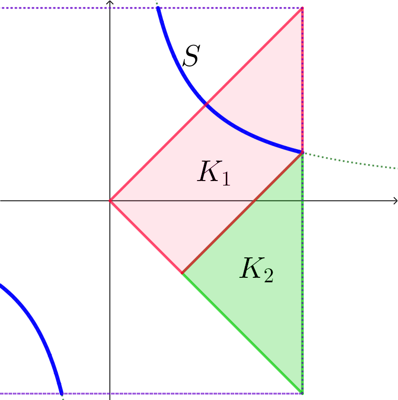
Case 1: .
In this case, we will traverse from to the in the direction . See Figure 14. First, consider the equation
in the variable and note the equality
Using the quadratic formula to solve for , we get
Note that the discriminant is nonnegative since
Set and note the identity . Therefore,
Observe now the equality
Hence it remains to bound . First we note that , since
In addition, since , we have . Since and are positive, we must therefore have . Thus, it remains to verify the bound . To that end, notice that
Therefore, . Since the function is increasing, we deduce .
Case 2: .
In this case, we will simply set . Define
Notice that proving the desired bound amounts to showing Observe the following estimates
where the the first inequality follows from the bounds and , second inequality follows from the bound , the equality follows from algebraic manipulations, and the third inequality follows from the estimate . Observe
Thus, by dividing through by , we need only show that
| (A.1) |
To prove this bound, note that since , we have the . Therefore, in the particular case when the estimate A.1 follows immediately. Define the linear function . Hence, assume Notice . Thus it suffices to show that the solution of the equation satisfies . To see this, we compute:
where the first inequality follows since and the second inequality follows since and , as desired. ∎
Now we prove the general case. First suppose that . Since and , we have
which proves the desired bound.
On the other hand, suppose that . Define the two vectors:
With this notation, we find that by Claim 1, there exists an satisfying , such that the following holds:
We now turn our attention to lower bounding the first term. Observe since , we have
Moreover, note the estimates, and , which imply that and . Thus, we obtain the lower bound
Finally, we obtain the bound
By recalling that , the proof is complete.
Appendix B Initialization
B.1 Proof of Proposition 5.1
As stated in Section 5, we first verify that and are nearby matrices with minimal eigenvectors equal to and . Then we apply the Davis-Kahan theorem [19] to prove that the minimal eigenvectors of and must also be close to the optimal directions.
Throughout the rest of the proof, we define the sets of “selected” inliers and outliers:
We record the relative size of these parameters as well, since they appear in the bounds that follow:
Theorem B.1.
Proof.
Without loss of generality, we only prove the result for ; the result for follows by a symmetric argument.
Define the projection operators and let Then decompose into the sums of four matrices , as follows:
| (B.1) |
We will now study the properties of these four matrices under both noise models.
First, note that in either case we may write , where
In addition, we will present a series of Lemmas showing the following high probability deviation bounds:
Finally, our bounds on the term as well as the definition of depend on the noise model under consideration. Thus, we separate this bound into two cases:
Noise model N1.
Under this noise model, we have
Thus, we set
Noise model N2.
Under this noise model, we have
Thus, we set
Therefore, under either noise model, the result will follow immediately from the following four Lemmas. We defer the proofs for the moment.
Lemma B.2.
There exist constants such that for any the following holds:
Lemma B.3.
For , we have
Lemma B.4.
There exist numerical constants such that for any we have
Lemma B.5.
The proof of the the theorem is complete. ∎
We now apply the Davis-Kahan theorem [19] as stated in Lemma C.1. Throughout we assume that we are in the event described in B.1.
Proof of Proposition 5.1.
We will use the notation from Theorem B.1. We only prove the result under N1, since the proof under N2 is completely analogous. Define matrices and . Matrix has spectral gap and top eigenvector , while matrix has spectral gap and top eigenvector . Therefore, since and , Lemma C.1 implies that
| and |
We will use these two inequalities to bound . To do so, we need to analyze and . We split the argument into two cases.
Suppose first . Then
as desired.
∎
The next sections present the proof of Lemmas B.2-B.5. We next set up the notation. For any sequence of vectors in , we will use the symbol to denote the vector in consisting of the last coordinates of .
We will use the following two observations throughout. First, by rotation invariance we will assume, without loss of generality, that and . Second, and crucially, this assumption implies that depends on only through the first component. In particular, we have that and are independent. Similarly, and are independent as well.
B.1.1 Proof of Lemma B.2
Our goal is to lower bound the quantity
To prove a lower bound, we need to control the random variables on the set .
Before proving the key claim, we first introduce some notation. First, define
which is strictly less than one since . Let and define to be the -quantile of the random variable . In particular, the following relationship holds
Additionally, define the conditional expected value
Rather than analyzing directly, we introduce the following set , which is simpler to analyze:
Then we prove the following claim.
Claim 2.
There exist numerical constants such that for all the following inequalities hold true:
- 1.
.
- 2.
- 3.
- 4.
Before we prove the claim, we show it leads to the conclusion of the lemma. Assuming we are in the event
it follows that
where the first three inequalities follow by the definition of the event . The fourth inequality follows by the definition of and Lemma C.13, which implies when and that the difference is minimized over at the endpoint . To get the claimed probabilities, we note that by Lemma C.13, we have for any setting of .
Now we prove the claim.
Proof of the Claim.
We separate the proof into four parts.
Part 1. By definition, we have
Part 2. By the definitions of and , the result will follow once we show that
To that end, first note that
where the first equality follows since , the first inequality follows since the minimum is taken over a smaller set, and the second inequality follows since the sum is taken over a smaller set of indices. Therefore, we find that
and our remaining task is to bound this probability.
To bound this probability, we apply Lemma C.9 to the i.i.d. sample , which is sampled from the distribution of of where and are independent. Therefore, using the identities (for )
and choosing , we find that
where we have used the identity in the first equality. This completes the bound and implies that with high probability, as desired.
Part 3. Since is an i.i.d. sample from the distribution of where are independent, we have for each , that
Therefore, . Finally, we apply Hoeffding’s inequality (Lemma C.3) to the i.i.d. Bernoulli random variables () to deduce that
as desired.
Part 4. First write
where first inequality follows from Part 2 and the bound . Thus, we focus on bounding the first term.
To that end, notice that
Observe that for any index and , we have , where are independent. In addition, we have , where we have used the fact that is an increasing function of . Therefore, applying Lemma C.10, we have the following bound:
where is a numerical constant. In particular, by Theorem C.7 and the identity , we have the following bound
for numerical constants and , as desired.
∎
The proof is complete. ∎
B.1.2 Proof of Lemma B.3
Our goal is to bound the operator norm of the following matrix:
Simplifying, we find that
Evidently, , so our focus will be to bound this quantity. We will bound this quantity through the following claim, which is based on Gaussian concentration for Lipschitz functions.
Claim 3.
Consider the (random) function , given by
Then is Lipschitz continuous and
Moreover, the following bound holds:
Proof of Claim.
For any and , we have
which proves that is -Lipschitz. Therefore, since for all the variables and are independent, standard results on Gaussian concentration for Lipschitz functions (applied conditionally), Theorem C.8, imply that
Thus, the first part of the claim is a consequence of the following bound:
We now turn our attention to the high probability bound on .
To that end, notice that the (random) function given by
is -Lipschitz continuous. Moreover, we have that Therefore, by Gaussian concentration we have
as desired. ∎
B.1.3 Proof of Lemma B.4
Observe the equality
Therefore, we seek to bound the following operator norm:
Using the tower rule for expectations and appealing to Corollary C.12, we therefore deduce
as desired.
∎
B.1.4 Proof of Lemma B.5
Noise model N1
Under this noise model, we write
The proof follows by repeating the conditioning argument as in the proof of B.4.
Noise model N2
B.2 Proof of Proposition 5.2
We will assume that . We will show that with high probability, , and moreover in this event if , we have . The other setting can treated similarly.
We will use the guarantees of Proposition 4.6. In particular, there exist numerical constants so that as long as , then with probability at least we have
and
Throughout the remainder of the proof, suppose we are in this event. Define the two univariate functions
By construction, if minimizes then minimizes Thus, to prove the claim we need only show that any minimizer of satisfies .
To that end, first note that and are close:
| (B.2) |
Therefore, setting , we obtain
where the second inequality follows from Theorem 4.6, the third inequality follows from Equation (B.2), and the fourth follows from the reverse triangle inequality. Thus, any minimizer of must satisfy
as desired. Finally suppose . Then we deduce . The proof is complete.
Appendix C Auxiliary Lemmas
C.1 Technical Results
This subsection presents technical lemmas we employed in our proofs. The first result we need is a special case of the celebrated Davis-Kahan Theorem (see [19]). For any two unit vectors , define .
Lemma C.1.
Consider symmetric matrices , where . Define to be the eigengap , and denote the first eigenvectors of by , respectively. Then
Additionally, we need the following fact about -nets over low-rank matrices, which we employ frequently to prove uniform concentration inequalities.
Lemma C.2 (Lemma 3.1 in [14]).
Let . There exists an -net (with respect to ) of obeying
C.2 Concentration Inequalities
In this subsection, we first provide a few well-known concentration inequalities about sub-gaussian and sub-exponential random variables.
Theorem C.3 (Hoeffding’s Inequality - Theorem 2.2.2 in [51]).
Let be independent symmetric Bernoulli random variables. Then for any , we have
Theorem C.4 (Bernstein’s Inequality - Theorem 2.8.4 in [51]).
Let be independent mean-zero random variables, such that for for all . Then for any , we have
here is the variance of the sum.
Theorem C.5 (Sub-gaussian Concentration - Theorem 2.6.3 in [51]).
Let be independent, mean zero, sub-gaussian random variables and Then, for every we have
where
Theorem C.6 (Sub-exponential Concentration - Theorem 2.8.2 in [51]).
Let be an independent, mean zero, sub-exponential random variables and let be a fixed vector. Then, for any we have that
where and is a numerical constant.
Theorem C.7 (Corollary 2.8.3 in [51]).
Let be independent, mean zero, sub-exponential random variables. Then, for every , we have
where is a numerical constant and .
Theorem C.8 (Theorem 5.6 in [9]).
Let be a vector of independent standard normal random variables. Let denote an -Lipschitz function. Then, for every , we have
The following concentration inequalities deal with quantiles of distributions:
Lemma C.9.
Let be an i.i.d. sample with distribution , choose to be the population quantile of the distribution , that is , and let be any probability with Then,
where denotes the -th quantile of the sample .
Proof.
It is easy to see that the following holds, if, and only if, . Notice that are i.i.d. Bernoulli random variables and thus Then, the result follows by applying Bernstein’s inequality (Theorem C.6) to . ∎
Lemma C.10.
Let be i.i.d. sub-gaussian random variables. For any such that , consider the random variable defined as conditioned on the event namely for all
Then, is a sub-exponential random variable, in other words for all we have that
where is the minimum scalar such that .
Proof.
Let us consider two cases. Suppose first . Then we have that and therefore the stated inequality is trivial.
Suppose now . Then we have that
With this we can bound the probability
as claimed. ∎
The following Theorem from [50] is especially useful in bounding the operator norm of random matrices:
Theorem C.11 (Operator norm of random matrices).
Consider an matrix whose rows are independent, sub-gaussian, isotropic random vectors in . Then, for every , one has
where depends only on .
Proof.
Let us record the following elementary consequence.
Corollary C.12.
Let be independent, sub-gaussian, isotropic random vectors in and let be an arbitrary set. Then, for every , one has
where depends only on .
Proof.
Consider the matrix whose rows are the vectors for . Then we deduce
Appealing to Theorem C.11, we therefore deduce for any the estimate
holds with probability . Now for any , choose such that, , namely Noting
completes the proof. ∎
Recall that we defined the functions and given as the -quantile of where are i.i.d. standard normal. Furthermore we defined
Lemma C.13.
The function given by
is nondecreasing. In particular, there exist numerical constants such that for any we have
where the tightest constants are given by and
Proof.
The bulk of this result is contained in the following claim.
Claim 4.
Let be arbitrary numbers, then
We defer the proof of the claim and show how it implies the lemma. Observe that the functions and are nondecreasing, thus it suffices to show that the function is nondecreasing. Let
where the inequality follows from the claim and the equalities follow from the identity for nonnegative random variables Hence is a nondecreasing function.
The above implies that for any we have . Note that is positive since it is defined by a positive integrand on a set of non-negligible measure. The bounds on and follow by a numerical computation. In particular we obtain that with the probability Then computing numerically (with precision set to 32 digits) we obtain Similarly we find that if we set we get Then evaluating we find
Proof of the claim.
The statement of the claim is equivalent to having that for any the function given by
is nonincreasing. Our goal is to show that In order to prove this result we proceed as follows. Define
and
Observe . Thus it suffices to show Invoking Leibniz rule we get
Repeating the same procedure we get Some algebra reveals we want to show
It is enough to show that the function is monotonically increasing. Define
Thus we have
Again, , hence we need to show After some algebra, this amounts to proving
The inequality is true if in particular the same holds for the integrands, i.e.
Since the previous inequality holds if
is increasing. By taking derivatives and reordering terms we see that this is equivalent to
Since is decreasing, we have
proving the claim. ∎
Thus the proof is complete. ∎