Optimal Network Control in Partially-Controllable NetworksThis work was supported by NSF Grant CNS-1524317 and by DARPA I2O and Raytheon BBN Technologies under Contract No. HROO l l-l 5-C-0097.
Abstract
The effectiveness of many optimal network control algorithms (e.g., BackPressure) relies on the premise that all of the nodes are fully controllable. However, these algorithms may yield poor performance in a partially-controllable network where a subset of nodes are uncontrollable and use some unknown policy. Such a partially-controllable model is of increasing importance in real-world networked systems such as overlay-underlay networks. In this paper, we design optimal network control algorithms that can stabilize a partially-controllable network. We first study the scenario where uncontrollable nodes use a queue-agnostic policy, and propose a low-complexity throughput-optimal algorithm, called Tracking-MaxWeight (TMW), which enhances the original MaxWeight algorithm with an explicit learning of the policy used by uncontrollable nodes. Next, we investigate the scenario where uncontrollable nodes use a queue-dependent policy and the problem is formulated as an MDP with unknown queueing dynamics. We propose a new reinforcement learning algorithm, called Truncated Upper Confidence Reinforcement Learning (TUCRL), and prove that TUCRL achieves tunable three-way tradeoffs between throughput, delay and convergence rate.
I Introduction
Optimal network control has been an active area of research for more than thirty years, and many efficient routing algorithms have been developed over the past few decades, such as the well-known throughput-optimal BackPressure routing algorithm [26]. The effectiveness of these algorithms usually relies on the premise that all of the nodes in a network are fully controllable. Unfortunately, an increasing number of real-world networked systems are only partially controllable, where a subset of nodes are not managed by the network operator and use some unknown network control policy, such as overlay-underlay networks.
An overlay-underlay network consists of overlay nodes and underlay nodes [3, 16, 19]. The overlay nodes can implement state-of-the-art algorithms while the underlay nodes are uncontrollable and use some unknown protocols (e.g., legacy protocols). Figure 1 shows an overlay-underlay network where the communications among overlay nodes rely on the uncontrollable underlay nodes. Overlay networks have been used to improve the capabilities of computer networks for a long time (e.g., content delivery [21]).

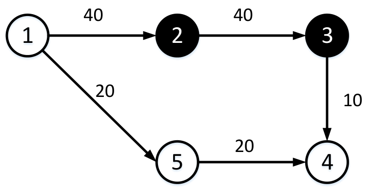
Due to the unknown behavior of uncontrollable nodes, the existing routing algorithms may yield poor performance in a partially-controllable network. For example, Figure 2 shows an example where the well-known Backpressure routing algorithm [26] fails to deliver the maximum throughput when some nodes are uncontrollable. In particular, uncontrollable node 3 adopts a policy that does not preserve the flow conservation law such that its backlog builds up, but uncontrollable node 2 hides this backlog information from node 1. As a result, if node 1 uses Backpressure routing, it always transmits packets to node 2, although these packets will never be delivered. A smarter algorithm should be able to learn the behavior of the uncontrollable nodes such that node 1 only sends packets along route .
As a result, it is important to develop new network control algorithms that achieve consistently good performance in a partially-controllable environment. In this paper, we study efficient network control algorithms that can stabilize a partially-controllable network whenever possible. In particular, we consider two scenarios.
First, we investigate the scenario where uncontrollable nodes use a queue-agnostic policy, which captures a wide range of practical network protocols, such as shortest path routing (e.g., OSPF, RIP), multi-path routing (e.g., ECMP) and randomized routing algorithms. In this scenario, we propose a low-complexity throughput-optimal algorithm, called Tracking-MaxWeight (TMW), which enhances the original MaxWeight algorithm [26] with an explicit learning of the policy used by uncontrollable nodes.
Second, we study the scenario where uncontrollable nodes use a queue-dependent policy, i.e., the action taken by uncontrollable nodes relies on the observed queue length vector (e.g., Backpressure routing). In this scenario, we show that the queueing dynamics become unknown and no longer follow the classic Lindley recursion [6], which makes the problem fundamentally different from the traditional network optimization framework: we not only need to know how to perform optimal network control but also need to learn the queueing dynamics in an efficient way. We formulate the problem as a Markov Decision Process (MDP) with unknown dynamics, and propose a new reinforcement learning algorithm, called Truncated Upper Confidence Reinforcement Learning (TUCRL), that is shown to achieve network stability under mild conditions.
I-A Related Work
Most of the existing works on network optimization in a partially-controllable environment are in the context of overlay-underlay networks. An important feature of overlay-underlay networks is that underlay nodes are not controllable and may adopt arbitrary (unknown) policies. The objective is to find efficient control policies for the controllable overlay nodes in order to optimize certain performance metrics (e.g., throughput). In [3], the authors showed that the well-known BackPressure algorithm [26], which was shown to be throughput-optimal in a wide range of scenarios, may lead to a loss in throughput when used in an overlay-underlay setting, and proposed a heuristic routing algorithm for overlay nodes called Overlay Backpressure Policy (OBP). An optimal backpressure-type routing algorithm for a special case, where the underlay paths do not overlap with each other, was given in [16]. Recently, [19] showed that the overlay routing algorithms proposed in [3][16] are not throughput-optimal in general, and developed the Optimal Overlay Routing Policy (OORP) for overlay nodes. However, all of the existing overlay routing algorithms [3, 16, 19] impose very stringent assumptions about the behavior of underlay nodes. In particular, the underlay nodes are required to use fixed-path routing (e.g., shortest-path routing) and maintain stability whenever possible, which fails to account for many important underlay policies (e.g., underlay nodes may use multi-path routing).
In terms of technical tools, our work leverages techniques from reinforcement learning, since a partially-controllable network with queue-dependent uncontrollable policy can be formulated as an MDP with unknown dynamics. Over the past few decades, many reinforcement learning algorithms have been developed, such as Q-learning [22], actor critic [4] and policy gradient [28]. Recently, the successful applications of deep neural networks in reinforcement learning algorithms have produced many deep reinforcement learning algorithms such as DQN [8], DDPG [5] and TRPO [20]. However, most of these methods are heuristic-based and do not have any performance guarantees. Among the existing reinforcement learning algorithms there are a few that do provide good performance bounds, such as model-based reinforcement learning algorithms UCRL [1, 2] and PSRL [15, 13]. Unfortunately, these algorithms require that the size of the state space be relatively small, which cannot be directly applied in our context since the state space (i.e., queue length space) contains countably-infinite states. In this work, we combine the UCRL algorithm with a queue truncation technique and propose the Truncated Upper Confidence Reinforcement Learning (TUCRL) algorithm that has good performance guarantees even with countably-infinite queue length space.
I-B Our Contributions
In this paper, we investigate optimal network control for a partially-controllable network. Whereas existing works (e.g., [3, 16, 19]) imposed very stringent assumptions about the behavior of uncontrollable nodes for analytical tractability, this is the first work that establishes stability results under the generalized partially-controllable network model. In particular, we develop two network control algorithms.
First, we develop a low-complexity Tracking-MaxWeight (TMW) algorithm that is guaranteed to achieve network stability if uncontrollable nodes adopt queue-agnostic policies. The Tracking-MaxWeight algorithm enhances the original MaxWeight algorithm [26] with an explict learning of the policy used by uncontrollable nodes.
Next, we propose a new reinforcement learning algorithm (i.e., the TUCRL algorithm) in the more challenging scenario where uncontrollable nodes may use queue-dependent policies. It combines the state-of-art model-based UCRL algorithm [1, 2] with a queue truncation technique to overcome the problem with countably-infinite queue length space. We prove that TUCRL achieves network stability by dropping a negligible fraction of packets. We also show that the TUCRL algorithm maintains a three-way tradeoff between delay, throughput and convergence rate.
II System Model
Consider a networked system with nodes (the set of all nodes is denoted by ). There are flows in the network and each node maintains a queue for buffering undelivered packets for each flow . As a result, there are queues in the network, and we denote by the queue length vector at the beginning of time slot , where its element represents the queue length for flow at node .
Let be the network event that occurs in slot , which includes information about the current network parameters, such as a vector of channel conditions for each link and a vector of exogenous arrivals to each queue. We assume that the sequence of network events follow a stationary stochastic process. In particular, the vector of exogenous packet arrivals is denoted by , where is the number of exogenous arrivals to queue in slot . Denote by the expected exogenous packet arrival rate to queue in steady state.
At the beginning of each time slot , after observing the current network event and the current queue length vector , each node needs to make a routing decision indicating the offered transmission rate for flow over link . The corresponding network routing vector is denoted by .
There are two types of nodes in the network: controllable nodes (the set of controllable nodes is denoted by ) and uncontrollable nodes (the set of uncontrollable nodes is denoted by ). The network operator can only control the routing behavior for controllable nodes while the routing actions taken by uncontrollable nodes cannot be regulated and are only observable at the end of each time slot. In this case, the network routing vector can be decomposed into two parts: . Here, represents the routing decisions made by controllable nodes (referred to as the controllable action) and corresponds to the routing decisions made by uncontrollable nodes (referred to as the uncontrollable action). The routing vectors and are constrained within some action spaces and , respectively, that may depend on the current network event , respectively. The action space for all nodes is denoted by . The action space can be used to specify routing constraints (e.g., the total transmission rate over each link should not exceed its capacity) or describe scheduling constraints (e.g., each node can only transmit to one of its neighbors in each time slot).
Note that when there is not enough backlog to transmit, the actual number of transmitted packets may be less than the offered transmission rate. In particular, we denote by (or simply if the context is clear) the actual number of transmitted packets in flow over link in slot under the current queue length . Clearly, we have . We further assume that the routing decision can always be chosen to respect the backlog constraints (but the actual actions may not necessarily be queue-respecting). This can be done simply by never attempting to transmit more data than we have. Under such notations, the queuing dynamics are given by
where . We also make the following boundedness assumption: the amount of exogenous arrivals and the offered transmission rate in each time slot are bounded by some constant , i.e.,
A network control policy is a mapping from the observed network event and queue length vector to a feasible routing action. In particular, denote by a controllable policy and an uncontrollable policy. In this paper, we assume that the uncontrollable policy remains fixed over time but is unknown to the network operator. Our objective is to find a controllable policy such that network stability can be achieved, as is defined as follows.
Definition 1.
A network is rate stable if
Rate stability means that the average arrival rate to each queue equals the average departure rate from that queue.
III Queue-Agnostic Uncontrollable Policy
In this section, we consider the scenario where the uncontrollable policy is queue-agnostic, which simply observes the current network event and makes a routing decision as a stationary function only of , i.e., . In the stochastic network optimization literature, such a policy is also referred to as an -only policy [11]. Despite their simple form, -only policies can capture a wide range of network control protocols in practice, such as shortest-path routing protocols (e.g., OSPF, RIP) , multi-path routing protocols (e.g., ECMP) and randomized routing protocols.
Unfortunately, even under simple -only uncontrollable policies, existing routing algorithms may fail to stabilize the network. For example, as is illustrated in Figure 2, the well-known Backpressure routing algorithm achieves low throughput when uncontrollable node uses queue-agnostic policies. In this example, the failure is due to the fact that some uncontrollable node uses a non-stabilizing policy that does not preserve flow conservation but the Backpressure algorithm is not aware of this non-stabilizing behavior.
In this section, we propose a low-complexity algorithm that learns the behavior of uncontrollable nodes and achieves network stability under any -only uncontrollable policy.
III-A Tracking-MaxWeight Algorithm
Now we introduce an algorithm that achieves network stability whenever uncontrollable nodes use an -only policy. The algorithm is called Tracking-MaxWeight (TMW), which enhances the original MaxWeight algorithm [26] with an explicit learning of the policy used by uncontrollable nodes. Throughout this section, we let be the sequence of routing actions that are actually executed by uncontrollable nodes.
The details of the TMW algorithm are presented in Algorithm 1. In each slot , the TMW algorithm generates the routing actions for controllable nodes and also produces an “imagined” routing action for uncontrollable nodes, by solving the optimization problem (2). With these calculated actions, the TMW algorithm then updates two virtual queues. The first virtual queue tries to emulate the physical queue but assumes that the imagined uncontrollable action is applied (while the physical queue is updated using the true uncontrollable action ). The second virtual queue tracks the cumulative difference between the imagined uncontrollable actions and the actual uncontrollable actions . In particular, we use to measure the difference between the imagined routing action and the true routing action taken by uncontrollable node , which is given by
| (1) |
where is the actual number of transmitted packets under the true routing action given the current queue backlog . Note that for each controllable node , we simply set .
The optimization problem (2) aims at maximizing a weighted sum of flow variables, which is similar to the optimization problem solved in the original MaxWeight algorithm [26] except for the setting of weights. In the original MaxWeight algorithm, the weight is corresponding to the physical queue backlog differential, while in the Tracking-MaxWeight algorithm the weight accounts for both the backlog differential for virtual queue and the backlog of virtual queue . The derivation of (2) is based on the minimization of quadratic Lyapunov drift terms for the two virtual queues:
where the first term corresponds to the Lyapunov drift of virtual queue and the second term is the Lyapunov drift of virtual queue . Note that the minimization is done over controllable actions and “imagined” uncontrollable actions . Cleaning up irrelevant constants, i.e., and , and rearranging terms yield the optimization problem (2).
| (2) |
Next we show that Tracking-MaxWeight achieves stability whenever uncontrollable nodes use an -only policy and the network is within the stability region, i.e., there exists a sequence of feasible routing vectors for controllable nodes such that
| (3) |
where
is the long-term average actual flow transmission rate under and is the corresponding optimal queue length trajectory. In other words, (3) requires that flow conservation should be preserved for every queue under the optimal controllable policy, otherwise no algorithm can stabilize the network. It is important to note that in (3) the flow conservation law is with respect to the actual transmissions since an uncontrollable node may not preserve flow conservation in terms of its offered transmissions (e.g., in Figure 2, the offered incoming rate to node 3 is 40 while the offered outgoing rate from node 3 is 0). The only way to stabilize these nodes is by limiting the amount of backlog such that the actual endogenous arrivals to these nodes are smaller. The performance of Tracking-MaxWeight is given in the following theorem.
Theorem 1.
When uncontrollable nodes use an -only policy and the network is within the stability region, Tracking-MaxWeight achieves rate stability.
Proof.
The proof first shows that the two virtual queues and can be stabilized by the TMW algorithm by using the Lyapunov drift analysis. Then we prove that whenever the two virtual queues are stable, the physical queue is also stable. See Appendix A for details. ∎
IV Queue-Dependent Uncontrollable Policy
The previous section investigated the scenario where uncontrollable nodes use a queue-agnostic policy (i.e., -only policy). In this section, we study a more general case where the uncontrollable policy may be queue-dependent, which can be used to describe many state-of-the-art optimal network control protocols. For example, the well-known Backpressure algorithm makes routing decisions based on the currently observed queue length vector. In this scenario, the uncontrollable policy is a fixed mapping from the observed network event and the observed queue length vector to a routing vector for uncontrollable nodes, i.e., .
Note that the queueing dynamics are
Since for each , its routing variable is an arbitrary (unknown) function of , the above queueing dynamics could depend on in an arbitrary (unknown) way that is not in the simple piecewise-linear form as in the classic Lindley recursion. As a result, we rewrite the queueing dynamics as
| (4) |
where is some unknown function that depends on our controllable routing action , the current queue length vector and the observed network event .
Due to the unknown queueing dynamics, many analytical tools for optimal network control break down. For example, the previous Tracking-MaxWeight algorithm utilizes the Lyapunov drift analysis which is not applicable if the queueing dynamics do not follow the Lindley recursion. As a result, optimal network control becomes very challenging and fundamentally different from the traditional stochastic network optimization framework. In the following, we first formulate the problem a Markov Decision Process (MDP) with unknown dynamics and then propose a new reinforcement learning algorithm that can achieve network stability under mild conditions.
Before moving on to the technical details, we first introduce some notations and assumptions that will be used throughout this section. For convenience, we define action and simply write “controllable routing action ” as “action ”, since the uncontrollable routing action has been implicitly treated as a part of the environment (see queueing dynamics (4)). For the same reason, “controllable policy ” and “policy ” are also used interchangeably. The action space for is denoted by which is assumed to be fixed and finite. We also make the following assumption regarding the optimal system performance.
Assumption 1.
There exists a policy such that with probability 1 for any , where is the queue length vector in slot under policy .
In other words, it is required that the total queue length should remain bounded under an optimal policy otherwise there is no hope for stabilizing the network. In essence, Assumption 1 requires that the network be stabilizable by some controllable policy .
IV-A MDP Formulation
We formulate the problem of achieving network stability as an MDP . Here is the routing action space for controllable nodes, and is the state space that corresponds to the queue length vector space . The cost function under action and state is given by , which corresponds to the sum of queue lengths in slot . In addition, is the state transition matrix, where is the probability that the next state is when action is taken under the current state . Note that the transition matrix is generated according to the queueing dynamics (4), and that the influence of network event and uncontrollable routing action has been implicitly incorporated into the probabilistic transition matrix . Note also that the queueing dynamics are unknown, so this is an MDP with unknown dynamics, which is also referred to as a Reinforcement Learning (RL) problem [23].
Let be the time-average expected total queue length when policy is applied in MDP and the initial queue length vector is , i.e.,
where the expectation is with respect to the randomness of the queue length trajectory when policy is applied in MDP . Also let be the minimum time-average expected queue length under an optimal policy . Our objective is to find an optimal policy that solves the MDP and achieves the minimum average queue length.
IV-B Challenges to Solving the MDP
The MDP has an unknown transition structure, which gives rise to an “exploration-exploitation” tradeoff. On one hand, we need to exploit the existing knowledge to make the best (myopic) decision; on the other hand, it is necessary to explore new states in order to learn which states may lead to lower costs in the future. Moreover, there might be some “trapping” sub-optimal states that take a long time (or is even impossible) for any policy to escape. Any algorithm that has zero knowledge about system dynamics at the beginning is likely to get trapped in these states during the exploration phase. Therefore, we need to impose restrictions on the transition structure in the MDP model. In particular, we restrict our consideration to weakly communicating MDPs with finite communication time, defined as follows.
Assumption 2.
For any two queue length vectors and (except for those which are transient under every policy), there exists a policy that can move from to within time slots (in expectation), where is a constant.
In other words, it is assumed that there is no “trapping” state in the system otherwise no reinforcement learning algorithm can be guranteed to avoid the traps and optimally solve the MDP. Note that in a weakly communicating MDP, the optimal average cost does not depend on the initial state (cf. [18], Section 8.3.3). Thus we drop the dependence on the initial state , and write the optimal average cost (queue length) as .
Another challenge is that the MDP has a countably-infinite state space (i.e., queue length vector space). Existing reinforcement learning methods that can handle such an infinite state space are mostly heuristic-based (e.g., [8][5][20]), and do not have any performance guarantees. On the other hand, there are a few reinforcement learning algorithms that do have good performance guarantees, but these algorithms require that the size of the state space be relatively small. Even if we consider a finite time horizon , the size of the queue length vector space could be up to (assuming bounded arrivals in each slot), which could lead to weak performance bounds. For example, in the UCRL algorithm [1, 2], the regret bound is , where is the size of the state space. If UCRL is applied in our context, the resulting regret bound would be which is a trivial super-linear regret bound.
IV-C TUCRL Algorithm
In this section, we develop an algorithm that achieves network stability under Assumptions 1 and 2. We call our algorithm Truncated Upper Confidence Reinforcement Learning (TUCRL), as it combines the model-based UCRL algorithm [1, 2] with a queue truncation technique that resolves the infinite state space problem.
Specifically, consider a truncated system where new exogenous packet arrivals are dropped when the total queue length reaches for some threshold . In such a truncated system, the state space is the truncated queue length vector space which contains all queue length vectors where the length of each queue does not exceed . In order for packet dropping to be feasible, we assume that there is an admission control action that can shed new exogenous packets as needed.
Our TUCRL algorithm applies the model-based UCRL algorithm [1, 2] in the truncated system, which maintains an estimation for the unknown queueing dynamics and then computes the optimal policy under the estimated dynamics. It applies the “optimistic principle” for exploration, where under-explored state-action pairs are assumed to be able to result in lower costs, which implicitly encourages the exploration of novel state-action pairs.
The detailed description of TUCRL is presented in Algorithm 2, which is similar to the standard UCRL algorithm except that queue truncation is applied when appropriate. Specifically, the TUCRL algorithm proceeds in episodes, and the length of each episode is dynamically determined. In episode , the TUCRL algorithm first constructs an empirical estimation for the transition matrix based on historical observations (step 1). In particular, the estimated transition probability from state to under action is
| (5) |
where is the cumulative number of visits to state-action pair up until the beginning of episode and is the number of times that transition happens up to the beginning of episode . Note that if , the estimated transition probability is set to be zero.
Then the TUCRL algorithm constructs an upper confidence set for all plausible MDP models based on the empirical estimation (step 2). The upper confidence set is constructed in a way such that it contains the true MDP model with high probability. Specifically, the upper confidence set contains all the MDPs with truncated queue length space and transition matrix where
| (6) |
Here, is the queue truncation threshold, is the starting time of episode and is a constant.
Next, the TUCRL algorithm selects an “optimistic MDP” that yields the minimum average queue length among all the plausible MDPs in the confidence set , and computes a nearly-optimal policy under MDP (step 3). The joint selection of the optimistic MDP and the calculation of the nearly-optimal policy are referred to an optimistic planning [9]. There are many efficient methods for performing optimistic planning, such as Extended Value Iteration [2] and OP-MDP [24]. For completeness, we provide a description of Extended Value Iteration in Appendix B.
Finally, the computed policy is executed until the stopping condition of episode is triggered. An episode ends when the number of visits to some state-action pair doubles, i.e., when we encounter a state-action pair such that its visiting frequency in episode () equals its cumulative visiting frequency up to the beginning of episode (). We will show that this stopping condition guarantees that the total number of episodes up to time is (see Appendix D). Note that during the execution of policy , new packet arrivals may be dropped if the total queue length exceeds . Here, the dropped packets could be any new arrivals to any queue. We will prove that the fraction of dropped packets is negligible if the threshold is properly selected.
IV-D Performance of TUCRL Algorithm
The following theorem characterizes the performance of the TUCRL algorithm regarding its queue length, packet dropping rate and convergence rate.
Theorem 2.
(Queue Length) The time-average expected queue length converges to a bounded value:
(Packet Dropping Rate) The long-term expected fraction of dropped packets is
where is the fraction of dropped packets within slots.
(Convergence Rate) The time-average expected queue length after slots is within a -neighborhood of the steady-state expected queue length, where is some polynomial in and is the big-O notation that ignores any logarithmic term.
Proof.
We first find an upper bound on the total queue length under TUCRL in the truncated system. Based on the queue length upper bound, we further analyze the fraction of time when queue truncation is triggered by using concentration inequalities. See Appendix C for details. ∎
There are several important observations regarding Theorem 2. First, the TUCRL algorithm achieves bounded queue length by dropping a negligible fraction of packets under a suitably large value of . Second, there is a three-way tradeoff between total queue length (delay), packet dropping rate (throughput) and convergence rate. For example, by increasing the value of , the packet dropping rate becomes smaller (i.e., throughput becomes higher) but the total queue length (delay) increases and the convergence becomes slower. Similar three-way tradeoffs between utility, delay and convergence rate are discussed in [7].
Complexity of TUCRL. The time complexity of TUCRL is dominated by the complexity of the optimistic planning module (step 3) which is implementation-dependent. For example, if a naive Extended Value Iteration (see Appendix B) is used, the time complexity of each value iteration step is exponential in the number of queues and thus cannot scale to large-scale problems. One way to scale the optimisic planning module is by using approximate dynamic programming that employs various approximation techniques in the planning procedure, such as using linear functions or neural networks to approximate the value function (see [17] for a comprehensive introduction). Recent deep reinforcement learning techniques may also be leveraged to efficiently perform value iterations in large-scale problems, such as Randomized Least-Squares Value Iteration (RLSVI) [14], Value Iteration Networks (VIN) [25] and Value Prediction Networks (VPN) [12]. Such approximations will not lead to significant changes in the performance of TUCRL since we only require an approximate solution in step 3.
V Simulation Results
V-A Scenario 1: Queue-Agnostic Uncontrollable Policy
We first study the partially-controllable network shown in Figure 3. There are two flows: and . Each node in the network needs to make a routing and scheduling decision in every time slot. The constraint is that each node can transmit to only one of its neighbors in each time slot and the transmission rate over each link cannot exceed its capacity. Node 2 and node 3 are uncontrollable nodes that use randomized queue-agnostic policies. Specifically, uncontrollable node 2 uses a randomized routing algorithm that transmits any packets it received to either node 3 or node 5 with an equal probability in each time slot. Uncontrollable node 3 uses a randomized scheduling policy that serves flow or flow with an equal probability in each time slot. The arrival rate of flow is 5. In this case, it can be shown that the maximum supportable arrival rate for flow is 25 given the routing constraints and the behavior of uncontrollable nodes.

We have shown in Section III that the Tracking-MaxWeight (TMW) algorithm achieves the optimal throughput in this scenario. In Figure 4(a), we compare Tracking-MaxWeight with the well-known MaxWeight algorithm (i.e., BackPressure routing), in terms of the supportable rate for flow . Specifically, Figure 4(a) shows the total queue length achieved by MaxWeight and Tracking-MaxWeight under different system loads (if the load is , then the arrival rate of flow is while the arrival rate of flow is fixed to 5). It is observed that MaxWeight can only support around 40% arrivals (the queue length under MaxWeight blows up at load ). By comparison, our Tracking-MaxWeight achieves the optimal throughput.
We further examine the behavior of the Tracking-MaxWeight algorithm in Figure 4(b) and Figure 4(c). Specifically, Figure 4(b) shows the queue length trajectory for the physical queue and the two virtual queues . As our theory predicts, both the physical queue and the two virtual queues are stable under the TMW algorithm. Figure 4(c) shows the learning curve of the TMW algorithm for the uncontrollable policy used by node . In particular, node uses randomized scheduling that serves flow and flow with an equal probability 0.5. It is observed in Figure 4(c) that the TMW algorithm quickly learns the service probability for flow at node 3 (i.e., the “imagined uncontrollable action” in TMW approaches the true uncontrollable action).
V-B Scenario 2: Queue-Dependent Uncontrollable Policy
Next we study a more challenging scenario where the action taken by uncontrollable nodes is queue-dependent. In particular, consider the network topology shown in Figure 5 where node 2 and node 3 are uncontrollable. There is only one flow and the constraint is that each node can transmit to only one of its neighbours in each time slot. The policy used by the two uncontrollable nodes is as follows. Let and be the transmission rate that node 2 and node 3 allocates to the flow in slot , respectively. Then
As a result, the maximum throughput of 1 can be supported only if is small () and is large (). Although this is an artificial example, it sheds light on the challenges when uncontrollable nodes use queue-dependent policies: any throughput-optimal algorithm should be able to efficiently learn which queue length region can support the maximum throughput and keep the queue length within this region.

We first compare the throughput performance of TUCRL with MaxWeight and Tracking-MaxWeight. Note that the TUCRL algorithm occasionally drops packets. In order to make a fair comparison, the throughput performance is measured with respect to the number of packets that have been delivered. It is observed in Figure 8 that TUCRL achieves the optimal throughput while MaxWeight or Tracking-MaxWeight only deliver a throughput of 0.5 in this scenario. It should be noted that the TUCRL algorithm takes longer time to learn and converge than MaxWeight or Tracking-MaxWeight.
Next we investigate the performance of the TUCRL algorithm under different values of the truncation threshold . As we proved in Theorem 2, the value of determines a three-way tradeoff between queue length, packet dropping rate and convergence rate. As is illustrated in Figure 8 and Figure 8, a larger value of leads to a larger queue length and the convergence becomes slower, but the fraction of dropped packets becomes smaller. Note that when and , the fraction of dropped packets becomes very small as time goes by. In contrast, when , the fraction of dropped packets remains non-negligible ( 60%) since the TUCRL algorithm cannot explore the “throughput-optimal region” where with a queue truncation threshold .
VI Conclusions
In this paper, we study optimal network control algorithms that stabilize a partially-controllable network where a subset of nodes are uncontrollable. We first study the scenario where the uncontrollable nodes use a queue-agnostic policy and propose a simple throughput-optimal Tracking-MaxWeight algorithm that enhances the original MaxWeight algorithm with an explicit learning of uncontrollable behavior. Then we investigate the scenario where the uncontrollable policy may be queue-dependent. This problem is formulated as an MDP and we develop a reinforcement learning algorithm called TUCRL that achieves a three-way tradeoff between throughput, delay and convergence rate.
References
- [1] Peter Auer and Ronald Ortner. Logarithmic online regret bounds for undiscounted reinforcement learning. In Advances in Neural Information Processing Systems, pages 49–56, 2007.
- [2] Thomas Jaksch, Ronald Ortner, and Peter Auer. Near-optimal regret bounds for reinforcement learning. Journal of Machine Learning Research, 11(Apr):1563–1600, 2010.
- [3] Nathaniel M Jones, Georgios S Paschos, Brooke Shrader, and Eytan Modiano. An overlay architecture for throughput optimal multipath routing. IEEE/ACM Transactions on Networking, 2017.
- [4] Vijay R Konda and John N Tsitsiklis. Actor-critic algorithms. In Advances in neural information processing systems, pages 1008–1014, 2000.
- [5] Timothy P Lillicrap, Jonathan J Hunt, Alexander Pritzel, Nicolas Heess, Tom Erez, Yuval Tassa, David Silver, and Daan Wierstra. Continuous control with deep reinforcement learning. arXiv preprint arXiv:1509.02971, 2015.
- [6] David V Lindley. The theory of queues with a single server. In Mathematical Proceedings of the Cambridge Philosophical Society, volume 48, pages 277–289. Cambridge University Press, 1952.
- [7] Jia Liu, Atilla Eryilmaz, Ness B Shroff, and Elizabeth S Bentley. Heavy-ball: A new approach to tame delay and convergence in wireless network optimization. In INFOCOM 2016-The 35th Annual IEEE International Conference on Computer Communications, IEEE, pages 1–9. IEEE, 2016.
- [8] Volodymyr Mnih, Koray Kavukcuoglu, David Silver, Alex Graves, Ioannis Antonoglou, Daan Wierstra, and Martin Riedmiller. Playing atari with deep reinforcement learning. arXiv preprint arXiv:1312.5602, 2013.
- [9] Rémi Munos et al. From bandits to monte-carlo tree search: The optimistic principle applied to optimization and planning. Foundations and Trends® in Machine Learning, 7(1):1–129, 2014.
- [10] Michael J Neely. Stability and capacity regions or discrete time queueing networks. arXiv preprint arXiv:1003.3396, 2010.
- [11] Michael J Neely. Stochastic network optimization with application to communication and queueing systems. Synthesis Lectures on Communication Networks, 3(1):1–211, 2010.
- [12] Junhyuk Oh, Satinder Singh, and Honglak Lee. Value prediction network. In Advances in Neural Information Processing Systems, pages 6120–6130, 2017.
- [13] Ian Osband, Daniel Russo, and Benjamin Van Roy. (more) efficient reinforcement learning via posterior sampling. In Advances in Neural Information Processing Systems, pages 3003–3011, 2013.
- [14] Ian Osband, Daniel Russo, Zheng Wen, and Benjamin Van Roy. Deep exploration via randomized value functions. arXiv preprint arXiv:1703.07608, 2017.
- [15] Yi Ouyang, Mukul Gagrani, Ashutosh Nayyar, and Rahul Jain. Learning unknown markov decision processes: A thompson sampling approach. In Advances in Neural Information Processing Systems, pages 1333–1342, 2017.
- [16] Georgios S Paschos and Eytan Modiano. Throughput optimal routing in overlay networks. In Communication, Control, and Computing (Allerton), 2014 52nd Annual Allerton Conference on, pages 401–408. IEEE, 2014.
- [17] Warren B Powell. Approximate Dynamic Programming: Solving the curses of dimensionality, volume 703. John Wiley & Sons, 2007.
- [18] Martin L Puterman. Markov decision processes: discrete stochastic dynamic programming. John Wiley & Sons, 2014.
- [19] Anurag Rai, Rahul Singh, and Eytan Modiano. A distributed algorithm for throughput optimal routing in overlay networks. arXiv preprint arXiv:1612.05537, 2016.
- [20] John Schulman, Sergey Levine, Pieter Abbeel, Michael Jordan, and Philipp Moritz. Trust region policy optimization. In International Conference on Machine Learning, pages 1889–1897, 2015.
- [21] Ramesh K Sitaraman, Mangesh Kasbekar, Woody Lichtenstein, and Manish Jain. Overlay networks: An akamai perspective. Advanced Content Delivery, Streaming, and Cloud Services, 51(4):305–328, 2014.
- [22] Richard S Sutton and Andrew G Barto. Reinforcement learning: An introduction, volume 1. MIT press Cambridge, 1998.
- [23] Richard S Sutton and Andrew G Barto. Reinforcement learning: An introduction, volume 1. MIT press Cambridge, 1998.
- [24] Balázs Szörényi, Gunnar Kedenburg, and Remi Munos. Optimistic planning in markov decision processes using a generative model. In Advances in Neural Information Processing Systems, pages 1035–1043, 2014.
- [25] Aviv Tamar, Yi Wu, Garrett Thomas, Sergey Levine, and Pieter Abbeel. Value iteration networks. In Advances in Neural Information Processing Systems, pages 2154–2162, 2016.
- [26] Leandros Tassiulas and Anthony Ephremides. Stability properties of constrained queueing systems and scheduling policies for maximum throughput in multihop radio networks. IEEE transactions on automatic control, 37(12):1936–1948, 1992.
- [27] Tsachy Weissman, Erik Ordentlich, Gadiel Seroussi, Sergio Verdu, and Marcelo J Weinberger. Inequalities for the l1 deviation of the empirical distribution. Hewlett-Packard Labs, Tech. Rep, 2003.
- [28] Ronald J Williams. Simple statistical gradient-following algorithms for connectionist reinforcement learning. In Reinforcement Learning, pages 5–32. Springer, 1992.
Appendix A Proof to Theorem 1
We first introduce a lemma that characterizes the load of the two virtual queues and .
Lemma 1.
There exists an -only controllable policy and an -only uncontrollable policy such that
where is the expected flow transmission rate under the -only policy or .
Proof.
Next we prove that the two virtual queues can be stabilized by the TMW algorithm.
Lemma 2.
Under the TMW algorithm, we have
Proof.
Define the Lyapunov function as
By the evolution of virtual queue , we have
where the inequality is due to the boundedness assumptions that and for any . Similarly, for virtual queue we have
where we rewrite as to explicitly emphasize on the dependence of on the imagined routing action , the true routing action and the current queue length .
As a result, the conditional expected Lyapunov drift can be bounded by
where the second inequality is due to the operation of TMW and is given in Lemma 1 which shows that
In addition, for any , when there are enough queue backlogs () we have
where is the queue length vector under the optimal controllable policy and the last equality is due to Lemma 1. As a result, when there are enough backlogs (i.e., for any ) we have
Let be the last time when there exists a queue such that , i.e., for any and any . Without loss of generality, we assume . Summing over and using law of iterated expectation, we have
It follows that
which implies that
Assuming that and , we have
Similarly, we have
This completes the proof. ∎
Finally, we show that as long as the two virtual queues and are stable, then the physical queue is also stable.
Lemma 3.
For any and , we have .
Proof.
We prove this lemma by induction on . The base case trivially holds true since we initialize and . Now suppose that holds true for some . Then for any we have
where the first inequality is due to the induction and simple algebra. Similar induction applies to every controllable node . This completes the induction proof. ∎
Appendix B Extended Value Iteration
In this appendix, we introduce Extended Value Iteration (EVI) [2] as one of the approaches for optimistic planning (see step 3 in Algorithm 2). Extended Value Iteration is similar to the canonical Value Iteration but applies to MDPs with “extended action space” where the additional action is the selection of the optimistic MDP (more precisely, the selection of the optimistic transition matrix) that yields the minimum average cost among a set of plausible MDPs. In particular, let be the value function for state obtained after iteration . Then Extended Value Iteration proceeds as follows. For any
| (7) |
where is given in (6). The inner minimization problem can be easily solved using the following greedy algorithm which tries to push as much probability mass to the state with the largest value.
Greedy Algorithm: find optimistic transition probability for a particular state-action pair
Input: Estimated transition probability and distance as given in (6)
1. Sort states in in descending order according to their value. We assume that the sorted state space is denoted by where
2. Set
3. Set
4. While do
(a) Reset .
(b) Set .
The distance in the input is the range used in our confidence set construction (6), i.e.,
The iteration stops when the following convergence criterion is triggered:
| (8) |
which requires that the span of the average cost across all states be less than or equal to .
Appendix C Proof to Theorem 2
We first introduce some notations.
- •
Let be an MDP model for the original untruncated system (where no packet dropping happens) with transition matrix . Denote by the true MDP model for the original untruncated system with the true transition matrix . Note that in an untruncated system, the state space is the countably-infinite queue length space .
- •
Let be a truncated MDP model with transition matrix for a truncated system with threshold . Note that the state space in a truncated MDP model is the truncated queue length space . Denote by the truncated true MDP model that is obtained by applying packet dropping to the original untruncated true MDP model .
- •
Let be the optimal time-average expected queue length in the untruncated true MDP . Similarly, denote by the optimal time-average expected queue length in the truncated true MDP .
The following theorem provides an upper bound on the total queue length in a truncated system with threshold .
Theorem 3.
With probability at least , the TUCRL algorithm achieves
| (9) |
where
Proof.
See Appendix E. ∎
Next, we provide an upper bound on the fraction of dropped packets based on Theorem 3.
Theorem 4.
When is sufficiently large, with probability at least , the fraction of dropped packets is
Proof.
See Appendix J. ∎
Note that the above results depend on the optimal average queue length in the truncated system. The following lemma shows the relationship between and (the optimal average queue length in the original untruncated system).
Lemma 4.
.
Proof.
See Appendix K. ∎
Combining Lemma 4, Theorem 3 and Theorem 4, we have that with probability at least the TUCRL algorithm achieves
and
On the other hand, the worst-case average queue length is at most and the worst-case packet dropping rate is 1, which happens with probability at most . As a result, the expected average queue length under TUCRL is
and the expected fraction of dropped packets is
For any given , taking and noting that (see Assumption 1) yield the desirable performance bounds in Theorem 2.
Appendix D Number of Episodes in TUCRL
The following lemma provides an upper bound on the number of episodes in TUCRL.
Lemma 5.
The total number of episodes in TUCRL up to time is bounded by
Proof.
Let be the set of episodes where the number of visits to a state-action pair is doubled up to the beginning of time , i.e.,
where is the index of the episode that contains time slot . Also let be the set of state-action pairs that have non-zero visits up to the beginning of episode . Then we claim that for any . Indeed, if , for any we have
which leads to a contradiction. As a result, we have
where the second inequality is due to the concavity of function. ∎
Appendix E Proof to Theorem 3
Define the regret (w.r.t. queue length) in episode as
where is the optimal average queue length for the truncated true MDP . Let be the number of episodes up to time (including the one that contains ). Without loss of generality, we assume that (i.e., is the end of episode ). Also denote by the set of episodes whose ending time is less than , and we similarly define . The regret up to time can be decomposed by
| (10) |
where the inequality is due to the fact the total amount of exogenous arrivals (and thus the total queue length) within the first slots is at most by our boundedness assumption. It turns our that the first term in (10) is of a lower order, and we focus on finding an upper bound on the second term. The following lemma shows that the constructed confidence set contains the truncated true MDP model with high probability.
Lemma 6.
For any , the probability that the truncated true MDP belongs to the confidence set for every episode is
Proof.
See Appendix F. ∎
In the following, we only consider the case where since this holds with high probability by Lemma 6. Let be the optimistic MDP selected in episode and define as the average queue length under MDP and the nearly-optimal policy . Note that by the accuracy requirement in Step 10 of the TUCRL algorithm. Moreover, due to the fact that the truncated true MDP and is the optimistic MDP that yields the minimum average queue length among all MDPs in , we have and thus
| (11) |
Then we can decompose as follows:
Summing over all episodes , we have
| (12) |
We first find an upper bound for the second term in the RHS of (12) by using Lemma 19 in [2]: for any sequence of numbers with , we have
As a result, defining and , we have
| (13) |
Then it remains to find an upper bound on the first term in the RHS of (12).
Lemma 7.
If for any , then with probability at least we have
Proof.
See Appendix G. ∎
Appendix F Proof to Lemma 6
The -deviation of the true distribution and the empirical distribution over distinct events from samples is bounded according to Weissman et al. [27] by
In our case, for each state-action pair , the number of possible next states is at most since the increase/decrease in the length of each queue is at most in every slot (including both exogenous and endogenous arrivals). Let be the transition probabilities for the truncated true MDP . Then the number of samples we obtained for distribution up to the beginning of episode (i.e., when ) is . As a result, for episode and any state-action pair such that , setting
guarantees that
| (14) |
Note that the above bound holds for every state-action pair such that . If there have not been any observations for some state-action pair , i.e., , the confidence intervals (6) trivially hold with probability 1. Thus, inequality (14) actually holds for every and .
Applying the union bound over all possible state-action pairs in the truncated MDP, we have for each episode
i.e.,
| (15) |
Let be the smallest episode index in . For any , we have . As a result, we have for any
where the first inequality is derived by applying union bound to (15), the second inequality is due to the definition of , the third inequality is due to Lemma 5 which states that the total number of episodes up to time is at most .
Appendix G Proof to Lemma 7
Note that can be re-arranged according to the visiting frequency for each state-action pair during episode :
As a result, we have
| (16) |
We first provide an observation regarding the value functions we derived in Extended Value Iteration (EVI) (7).
Observation 1.
If the truncated true MDP belongs to the confidence set , then for any iteration in EVI, the range of the derived value function is bounded by , i.e.,
| (17) |
Proof.
Note that in the th iteration of EVI, the derived value function is the sum of expected queue lengths within time steps under an optimal (possibly non-stationary) -step policy starting in state in the MDP with extended action set (the extra action is to select an MDP within ). If there are two states such that , then an improved value for state could be achieved by adopting the following policy. First, follow a policy which always selects the truncated true MDP (this is a feasible action in the extended action set by our assumption) and moves from to most quickly in , which takes at most steps on average by Assumption 2. After reaching state , we follow the optimal -step policy for for the remaining time steps. Note that the sum of accumulative queue lengths before reaching state is at most since in each time step the total queue length is at most in the truncated system. As a result, the constructed policy yields , contradicting our assumption that . ∎
It is a direct consequence of Theorem 8.5.6. of [18], that when the convergence criterion (8) holds at iteration , then
| (18) |
In the following, letter will be reserved to reference the iteration where the convergence criterion (8) is triggered. Expanding according to (7), we have
and hence by (18) we have
which implies that for any
where the second equality holds because .
Define (we use the subscript to reference the episode). It is clear from Observation 1 that . Then we can rewrite the above inequality as
| (19) |
As a result, we have
| (20) |
To simplify notations, we define a row vector , a column vector and a matrix . Then (20) can be rewritten as
| (21) |
The second term in the RHS of (21) can be further decomposed as follows:
| (22) |
where is the transition matrix if we apply policy in the truncated true MDP model . Summing over all episodes , we have
| (23) |
Simarly, by Lemma 19 in [2], the first term in the RHS of (23) can be bounded by , which is a lower-order term. Next we find upper bounds for the last two terms in the RHS of (23), given in the following two lemmas.
Lemma 8.
with probability at least .
Proof.
See Appendix H. ∎
Lemma 9.
.
Proof.
See Appendix I. ∎
Appendix H Proof to Lemma 8
We find an upper bound for . We first define a suitable martingale and make use of the Azuma-Hoeffding inequality.
Lemma 10 (Azuma-Hoeffding inequality).
Let be a martingale difference sequence with for all . Then for any and ,
Define a -dimensional vector where the coordinate corresponding to state being 1 and all other coordinates being 0. Let be the sequence of states and actions up to slot , and let be the episode containing slot . Consider the sequence
where is the action taken by the TUCRL algorithm in slot . Note that conditioned on the historical sequence , the randomness of is in the next state . Also, is a sequence of martingale differences since for all . In addition, we have .
Then we have
where the last inequality is due to . Let be the set of slots contained in episodes . By the Azuma-Hoeffding inequality, we have
Summing over , we have with probability at least
where we use the fact that and (see Lemma 5).
Appendix I Proof to Lemma 9
We find an upper bound for . Since both the truncated true MDP and the selected optimistic MDP are in the confidence set , the term can be bounded using the confidence set construction (6). We have
| (24) |
where is the transition matrix for the truncated true MDP and we use the fact that .
Let such that . Moreover, recall that , and that by the stopping condition of episode . As a result, we have
Here we used for the second inequality that
where and (see Lemma 19 in [2]), and we used Jensen’s inequality for the last inequality. Finally, by the definition of and we have
which completes the proof.
Appendix J Proof to Theorem 4
Let be the set of slots when . Note that the amount of exogenous arrivals to each queue is at most in each time slot, and thus packet dropping occurs in a slot only if . As a result, in order to bound the amount of dropped packets, we find an upper bound for .
Note that
By Theorem 3, with probability at least , the TUCRL algorithm achieves
which implies that
| (25) |
Since at most packets are dropped for each slot , the amount of dropped packets within slots is at most
Note that the amount of total exogenous arrivals in each slot is i.i.d. with expectation , and . By Hoefdding’s inequality, we have
When , the above probability is less than . As a result, with probability at least , the fraction of dropped packets is at most
Appendix K Proof to Lemma 4
By Assumption 1, we have that for any
for some constant . Then it follows that for any
By Bounded Convergence Theorem, we have
As a result, we have
By Markov inequality, we have
As a result, with probability at least , the optimal policy never visits any queue length vector outside and the optimal average queue length is not affected in the truncated MDP, i.e., , which implies that .