Center of Gravity-based Approach for Modeling Dynamics of Multisection Continuum Arms∗
Abstract
Multisection continuum arms offer complementary characteristics to those of traditional rigid-bodied robots. Inspired by biological appendages, such as elephant trunks and octopus arms, these robots trade rigidity for compliance, accuracy for safety, and therefore exhibit strong potential for applications in human-occupied spaces. Prior work has demonstrated their superiority in operation in congested spaces and manipulation of irregularly-shaped objects. However, they are yet to be widely applied outside laboratory spaces. One key reason is that, due to compliance, they are difficult to control. Sophisticated and numerically efficient dynamic models are a necessity to implement dynamic control. In this paper, we propose a novel, numerically stable, center of gravity-based dynamic model for variable-length multisection continuum arms. The model can accommodate continuum robots having any number of sections with varying physical dimensions. The dynamic algorithm is of complexity, runs at 9.5 kHz, simulates 6-8 times faster than real-time for a three-section continuum robot, and therefore is ideally suited for real-time control implementations. The model accuracy is validated numerically against an integral-dynamic model proposed by the authors and experimentally for a three-section, pneumatically actuated variable-length multisection continuum arm. This is the first sub real-time dynamic model based on a smooth continuous deformation model for variable-length multisection continuum arms.
Index Terms:
continuum arms, dynamics, center of gravity, real-timeI Introduction
School of Computing, DePaul University, Chicago, IL 60604. email: igodage@depaul.edu. Dept. of Mechanical Engineering, Vanderbilt University, Nashville, TN 37212. Dept. of Electrical and Computer Engineering, Clemson University, SC 29634.
This work is supported in part by the National Science Foundation grant IIS-1718755. Submitted to IEEE Transactions on Robotics.
Rigid-bodied robots have been the backbone of the robotic industrial revolution which has not only significantly improved throughput but also relieved humans of most of the mundane, repetitive, dangerous, and dirty tasks of assembly lines. Rigid-linked industrial robots have high payload capacity and precision superior to human capabilities. However, the lack of compliance of rigid robots renders them dangerous and therefore industrial robot task-spaces are often restricted of human presence. In addition, due to the structural rigidity, they are poorly adaptable to environmental interaction and yield poor performance in unstructured environments [1]. There is currently great interest in robots that work cooperatively with humans [2], which implies a need for inherently human-safe robotic manipulators. Continuum robots have been proposed as a potential solution to serve niche applications where adaptability, compliance, and human safety are critical [3]. In this paper, we refer to continuum robots as those robotic structures that lack rigid frames and generate motion through smooth, continuous structural deformation, such as the robots reported in [4, 5, 6, 7, 8, 9].


Continuum arms are inspired by biological appendages such as elephant trunks and octopus arms. Made entirely out of muscle fibers, continuum arms structures are highly deformable to achieve complex geometrical shapes. Despite being made entirely out of muscles, they demonstrate compelling benchmarks in terms of forces and precision of operation [12, 13, 14, 15, 16]. Often constructed from elastic material, continuum arms aim to imitate such behavior by generating complex smooth geometric shapes through structural deformation. The smaller continuum robots target operation in smaller spaces such as inside human bodies during minimally invasive surgeries [17], and are actuated by elastic tubes or tendons. The larger variants, constructed to handle macro or human body scale objects are often powered by pneumatic muscle actuators (PMA). PMA’s, also known as McKibben actuators have number of desirable features, such as ease of design, fabrication, and high power-to-weight ratio, and therefore are sought after in continuum arm designs. In this paper we focus on PMA powered variable-length multisection continuum arms. There are several key features common to this type of manipulator. Unlike tendon-actuated continuum arms, they are fabricated by serially stacking continuum sections where each continuum section consists of multiple PMAs (typically three, though four actuators are also possible [6]) and are capable of generating omindirectional bending deformation independent of other sections. Since there are no backbones, continuum sections undergo axial length changes, extend or contract, depending on the PMA operation mode. Figures 1a and 1b show a couple of variable-length multisection continuum arm prototypes. Due to their unique mechanical characteristics, deriving mathematical models for these robots has been a challenge.
I-A Prior Work on Dynamic Modeling of Continuum Arms
Early continuum-style (which are not truly continuum without continuously bending deformation) robots have been discretized rigid structures [18, 19] that mimicked smooth bending. The computational constraints that prevailed at the time motivated numerically efficient parametric or modal approaches [20]. However, such low dimensional methods did not fully capture the complete task-space and suffered from numerical instabilities [21]. Other early continuum-style robots and discrete-link dynamic models include [14, 22, 5].
Cosserat rod theory has been proposed to model quasi-statics of tendon actuated inextensible flexible backbone and concentric continuum robots [23, 24, 6]. The work in [6] employed a similar approach to model the dynamics of a multibending soft manipulator but, owing to the complexity associated with highly deformable bodies, reported inefficient simulation times. The work reported in [25] utilized elliptic integrals to develop kinematics and statics of miniature single continuum section. Dynamics based on Kane’s method was reported in [26] to model the dynamics of a tendon-actuated continuum manipulator. The work in [27] proposed and validated a planar and static Cosserat rod model for PMA actuated variable-length multisection continuum sections, but the approach has not been extended for modeling spatial dynamics.
Another avenue to derive equations of motion (EoM) is to utilize energy-based methods such as the Lagrangian formulation. During operation, the relative displacement between points of a continuum body varies and thus limits the use of numerically efficient algorithms [28]. Theoretical models for inextensible, unidimensional, rope-like mechanisms were proposed in [29], but continuum arms have multiple degrees of freedom (DoF).
The kinematic model reported in [30] laid the foundation for curve parametric models for variable-length continuum arms. Nonetheless, the use of circular arc parameters resulted in complex nonlinear terms and numerical instabilities for straight-arm poses to limit the model’s extensibility for modeling dynamics. For an in-depth treatment of the limitations of curve parametric models, see [10]. An energy-based derivation of planar dynamic models for OctArm variable-length continuum manipulator [11] were reported in [31, 32]. However, continuum arms are capable of spatial operation, and the models were not experimentally validated. In addition, the resulting EoM were nonlinear, complex, and of integral nature, and therefore numerically inefficient and unstable.
Prior work by the first author proposed a modal method to overcome the numerical instabilities and inefficiencies present in curve parametric models. Therein, the terms of the homogeneous transformation matrix (HTM) of continuum sections were approximated by multivariate polynomials [33, 10] where the degree of polynomials could be chosen to meet desired error metrics. The model laid the foundation for formulating EoM of variable-length continuum sections [34, 35, 36]. The extended recursive formulation was later validated for a variable-length multisection continuum manipulator [37]. Therein, the integral terms are presolved to improve the numerical performance.
Numerically efficient (via rigid body dynamic algorithms) lumped models have also been applied for continuum robots. However, such models require a large number of discrete joints to approximate the deformation [38, 22, 14]. Some work has attempted to trade numerical efficiency for modeling accuracy by using relatively few rigid segments [39, 40].
The key motivation of this paper is to introduce a lumped model without betraying the continuous nature of the resulting expressions. Our prior work introduced a center of gravity (CoG) based modeling approach for a single continuum section [41, 42]. Therein, the EoM were derived for a point mass at the CoG of the continuum section. Thus, instead of an integral formulation, the process resulted in a compact model and superior numerical efficiency. In the derivation process, due to the physical dimensions of the robot, we did not consider the angular kinetic energy as the energy contribution was less than 3%. But this will not be the case for all continuum arms. In addition, the model was limited to a single continuum section where continuum arms with multiple sections are required for performing useful tasks such as whole arm manipulation [43]and spatial trajectory tracking [33].
I-B Contribution
In this work, we extend and generalize our CoG-based spatial dynamic model derived for a single continuum section [42], evaluate against the integral dynamics proposed in [37] to verify the numerical accuracy and computational efficiency, and validate the model against spatial dynamic responses of the prototype arm shown in Fig. 1a. Beyond our prior work reported in [37, 42, 41], the proposed dynamic model; (1) accommodates variable-length multisection continuum arms with arbitrary number of sections and a wide range of length and radii combinations, (2) considers both linear and angular kinetic energies of the continuum arm at the CoG for better system energy accuracy, (3) achieves energy matching via a series of energy shaping coefficients that are constant for any variable-length multisection continuum arms, (4) employs the results from [37] to systematically derive the EoM terms recursively, (5) demonstrates complexity for the first time for a dynamic model based on continuous (non-discretized) deformation representation, and for a three-section continuum arm, (6) runs at 9.5 kHz (step execution rate), and (7) achieves sub real-time dynamic simulation in Matlab Simulink environment. Therefore the proposed model unifies the ideas of lumped parametric approaches of discrete rigid-bodied robotics and continuous (integral) approaches of continuum robotics and is expected to lay a strong numerical and algorithmic foundation for implementing dynamic control schemes.
II Kinematics of Centers of Gravity
II-A System Model and Assumptions
Tables I and II list the nomenclatures of mathematical symbols and operators employed in this paper. Figure 2a shows the schematic of a multisection continuum arm with sections. The sections are numbered starting from the base continuum section (index 1) attached to the task-space coordinate system, . Any continuum section (Fig. 2b) is assumed to be actuated by three extending PMAs which are mounted on plates situated at either end at distance from the neutral axis and rad apart. Let the unactuated length of PMAs be , the maximum length change , and the joint-space vector of the continuum section, where . The joint where the continuum section is attached introduces linear displacement along and angular displacement about the +Z axis of . As the PMAs are constrained to maintain clearance normal to the neutral axis, differential length changes cause the section to bend or extend (when length changes are equal) [11]. The subsequent derivations rely on the assumptions that the continuum sections bend in circular arc shapes, have constant mass , and uniform linear density11 1 These are reasonable assumptions under typical operating conditions without large external forces as shown in [10] and [37]..
| Symbol | Definition |
|---|---|
| Continuum section index♯. | |
| Refers to the center of gravity-related terms | |
| , , | Radius, original length, and actuator length change |
| ,, | Complete, , and up to section joint space vector∗ |
| ,, | Task, base, and moving coordinate frames |
| ,, | HTM‡, position, and rotation matrices relative to |
| ,, | HTM, position, and rotation matrices relative to |
| Scalar to define along the continuum section | |
| Mass of continuum section | |
| , | Total and section kinetic energy |
| , | Angular and linear kinetic energies of continuum section |
| , | Total and section potential energy |
| , | Disc linear and angular inertia matrices |
| , | Complete inertia and Coriolis/Centrifugal matrices |
| , | Generalized linear and angular inertia matrices |
| , | Linear, angular Coriolis/Centrifugal force matrices |
| , | Complete, section conservative force vectors |
| , | Linear velocity Jacobian and Hessian w.r.t to |
| , | Angular velocity Jacobian and Hessian w.r.t to |
| Elastic stiffness coefficient matrix | |
| Complete input force vector in the joint space | |
| Rank 3 identity matrix |
Subscript represents the continuum section parameters whereas superscript stands for terms associated with up to the continuum section.
Lowercase, boldface italics (i.e., ) denote vectors and regular lowercase italics (i.e., or ) denote vector/matrix elements or constants. Matrices are denoted by boldface uppercase letters (i.e., , )
Homogeneous transformation matrix (HTM).
All quantities are represented in metric units.
| Operator | Definition |
|---|---|
| Partial derivative with respect to elements of along the dimension of . Eg. if and , then and respectively. | |
| Forms the velocity vector from skew-symmetric angular velocity matrix | |
| Integration from 0 to 1 with respect to | |
| Trace operator (involving only the first two diagonal elements) on a matrix or sub-matrix |


II-B Recursive Velocities, Jacobians, and Hessians
The kinematics of continuum arms has been well studied over the years [17, 30, 44, 45]. The proposed work uses the modal kinematics [10] for subsequent derivation of the EoM. This section provides a review of the modal kinematics for multisection continuum arms. A detailed exposition of kinematics is found in [10].
The deformation of a continuum section can be defined by the curve parameters radius of the circular arc, angle subtended by the circular arc, and 22 2 As shown in [10], the curve parameters are also functions of unactuated length of PMAs, , and radius of continuum section, , but are not included in the notation (constants for a given continuum arm) for brevity. (see Fig. 2b). Employing the curve parameters, the HTM of along the neutral axis of the continuum section at with respect to , , is computed as
where , and are HTM that denotes translation along the +X axis, rotation about the +Z and +Y axes respectively. is the resultant rotation matrix and is the position vector. The scalar denotes any point along the neutral axis where is the base where and is the tip of the continuum section. We then apply order multivariate Taylor series expansion on the terms of (II-B) to obtain numerically efficient and stable modal form of the HTM (see [10]).
Employing the continuum section HTM given in (II-B) and principles of kinematics of serial robot chains, the HTM of any section with respect to the task-space coordinate system , , is given by
where and define the position and orientation of along the neutral axis at of the continuum section.
The HTM in (II-B) can be expanded to obtain the recursive form of the kinematics as
| (5) | ||||
where and is the section tip rotation matrix and position vector of the preceding continuum section. Notice the absence of as as per the definition of (see [10]). Also, from now on, the dependency variables are not included in the equations for reasons of brevity.
Exploiting the integral Lagrangian formulation [37], we consider a thin disc at (which lies on the XY plane of . Utilizing (5), the angular and linear body velocities with respect to , and respectively, can be defined as
| (6) | ||||
where we define and for ease of subsequent development of the EoM, The derivations are outlined in appendices A-A2 and A-A1.
As shown in [37], Jacobians and Hessians play a critical role in recursive development of the EoM. Applying the standard techniques, the angular and linear velocity Jacobians, and respectively are derived. Here also, we use the property to define , in the development of the EoM and it is given by
where and and . Appendix A-A3 details the derivation.
Taking the partial derivative of (II-B) with respect to , the angular body velocity Hessian, is given by
where . Refer to Appendix A-A5 for the derivation.
Similarly, the linear velocity Jacobian, , and Hessian, are given by
II-C Extension for Kinematics of Centers of Gravity
Similar to Section II-B, without losing generality, we derive the kinematics for the CoG of any section . We define a coordinate system at the CoG, , whose HTM, , with respect to is defined as
where is the resultant rotation matrix and is the position vector [41]. Note that the CoG is a function of and therefore varies as the continuum section deforms.
To derive the kinematics of the CoG coordinate frame, , with respect to , we can combine with the general HTM given in (II-B). From the definition, (Fig. 2b) and therefore, CoG of the section relative to , , can be defined as
where is orientation and are position matrices of the CoG coordinate frame.
Analogous to (5), the recursive form of and are given by
| (19) | ||||
where and are formulated from (5).
Similar to (6), the angular and linear body velocities of the CoG (relative to ), and can be derived as
| (20) | ||||
where and , defined in (6), are linear and angular velocities at the tip of the continuum section. Here too, we employ the relationship . to compute .
Akin to (II-B), (II-B), (II-B), and (II-B) the angular body velocity Jacobian of CoG, , Hessian , linear body velocity Jacobian , , Hessian , are respectively given by (II-C), (II-C), (II-C), and (II-C) as
II-D Case Study: Point vs. Non-point Mass at the CoG
Consider the CoG velocities depicted in (20) when with , , , and . Physically this refers to a non-actuating continuum section (essentially a cylinder of length and radius whose CoG is located at the mid point, i.e., , of the neutral axis where the tip of the section rotates in place without translation. This scenario is theoretically possible and demonstrated in [10] where kinematic decoupling is present in multisection continuum arms. From (20), the CoG velocities become and . The kinetic energies of the section then become and . If a point-mass is considered at the CoG, it will result in . As a result, it becomes evident that a point-mass model is not suitable for modeling multisection continuum arms. Thus, in this paper, we will consider a hypothetical thin disc of mass and radius on the XY plane of with its geometric center coinciding the origin of , i.e., at the CoG (Fig. 2b). The respective kinetic energies then become and to match that of the actual continuum section energy. Employing the disc model at the CoG, following section derives the energy shaping coefficients [41] to match energies to that of the integral model reported in [37].
III Derive Energy Balance of Center of Gravity-based System
III-A Continuum Section Kinetic Energy: Integral and CoG-based Models
Without losing generality, we next derive the kinetic energies, angular and linear, for any continuum section. Then we compare the terms to formulate the energy scaling conditions. Analogous to [37], to find the kinetic energy of the continuum section using an integral approach, we will consider an infinitesimally thin disc of radius along the length of the continuum section. By applying the body velocities given by equations (6), the energy computed for a disc is then integrated with respect to to compute the section energy. The angular kinetic energy, , is given by
| (29) |
where is the moment of inertia about the X axis of .
Using the angular velocity given in (20), finding the angular kinetic energy of the disc at the CoG, , results in
| (30) | ||||
Similarly, using the linear body velocity in (6), the linear kinetic energy of the continuous model, , can be computed as
| (31) | ||||
where . Additionally, the CoG model’s linear kinetic energy, , is derived as
| (32) |
III-B Minimize Energy Difference Between the Integral and CoG-based Models
In this section, utilizing the energies derived in Section III-A, we systematically derive scalars to match the kinetic energy of the CoG models to that of the integral model. Unlike the single section case [41] however, the kinetic energy is dependent on the velocities of the section as well as the previous sections. Consider the angular energy difference between the models, derived for the continuum section, given by
| (33) |
where are the energy shaping coefficients that we apply to the CoG energy terms to match the energies.
Note that, in this case, unlike the single section case [42], we have three terms that do not get canceled when taking the difference. Likewise, the linear kinetic energy difference is computed as
| (34) |
Notice that some terms are canceled due to the absence of products of integrable terms, and thus resulting in three remaining terms. We introduce the energy shaping coefficients, , for each of those terms. The coefficients, introduced in (33) and (34), will be solved in the latter part of this section through a multivariate optimization routine.
III-B1 Generate Random Sample Set
Including the physical robot parameters such as , , and , the energy differences given by (33) and (34), become functions of where and are the normalized length and radius of the continuum section. Similarly, we generate random combinations of , , , and . The upper bound of limits maximum bending angle of continuum sections to . Also, note that depends on , and for a general section, it is not possible to sample the joint-space variables since is arbitrary. To overcome this challenge, we generate random where each component is chosen from the range . Note that these parametric bounds for and , though arbitrary and unrealistically large for physical continuum arms, were chosen to ensure the rigor and generality of the proposed model and within the error bounds of the order modal shape functions used in this paper. However, one may increase this bound (which would also require adjusting the order of modal shape functions of the HTM elements to meet the desired position and orientation error metrics at the tip at the maximum bending). More details related on choosing expansion order and errors can be found in [10].
III-B2 Computing the Energy Shaping Coefficients
For the random combinations of joint-space variables and physical parameters generated in the previous step, corresponding kinetic energy differences of the integral and CoG-based models, depicted in (33) and (34) are computed. As suggested by the definitions, for the ease of comparison of corresponding terms, we computed the three residual terms of each of kinetic energy differences separately. For instance, in the case of , terms , , and are computed separately. Similarly, for , , , and are computed separately. Then the sum of these terms, scaled by , will yield the energy difference, . The same approach is followed for the linear kinetic energy difference given by (34) and scaled by . The corresponding terms for the integral system and the CoG-based system are then plotted against each other in Fig. 3.
It can be seen that, despite the variation of the physical shape ( and ), there are proportional relationships between the matching terms of the two analytical models. This indicates us that the fundamental variable-length continuum section behavior across the two systems are proportional and independent of the physical shape. The proportional constants can be computed in two ways. One approach is to consider matching terms individually and compute the least square linear fit. The other approach is to consider the entire system’s kinetic energy and find the optimal coefficients that would minimize the cumulative energy difference. In this work, we have opted for the latter approach, since it provided a slight, though negligible, improvement in energy matching. We formulated our optimization problem in Matlab 2017a and used global optimization on the inbuilt fmincon multivariate constrained optimization subroutine using the objective function for all the parametric combinations. Noting the direct proportionality, we bounded the scalar range to for numerical efficiency. The resultant energy shaping coefficient values are shown in Fig. 3.
Notice that the proportional coefficient of Fig. 3f is slightly more aggressive than what the data suggests. The reason is the difference of the ratio of contributions from individual terms. For instance, the contribution of the term is orders of magnitude greater than that of the term . The system-wide energy consideration would then place more emphasize on larger contributors to yield optimal energy scalars, and this explains the sub-optimal results of the term-wise computation of proportional coefficients. However, based on our computations, given the strong correlation of the energy terms between the two modeling approaches, either method produces sufficient accuracy for practical purposes.


III-B3 Numerical Validation of Energy Shaping Coefficients
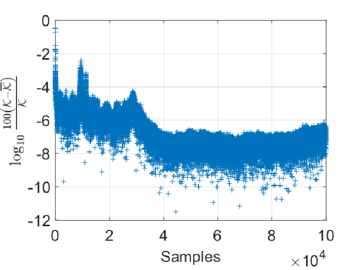
In this section, we statistically validate the coefficients generated in the previous section for a ten-section continuum robot model. For an section continuum arm, variables are required to compute the kinetic energy ( joint-space displacements and velocities). Assuming the , , and (physical parameters corresponding to the prototype arm shown in Fig. 1a), here we generate samples of uniformly distributed values within and for and respectively for the continuum arm numerical model. The difference of the complete system kinetic energies is computed by taking the cumulative of section-wise energy differences given by (33) and (34). The energy difference percentages, normalized to , for each sample, are then computed and plotted in Fig. 4a. Note that, , is not the absolute maximum kinetic energy for the given robot, but rather it is a statistical upper bound, and therefore the energy error percentages computed here are conservative, and the actual error is likely to be significantly lower in practice. The error percentage distribution is shown in Fig. 4b. The figure shows that the energy difference is essentially negligible with mean error percentage. The results show that the computed energy scalars are accurate and applicable for arbitrary length continuum arms without undesirable error propagation, eliminating the need for complex integral terms.

III-C Potential Energy of Continuum Sections
As reported in [37], a continuum arm is subjected to gravitational and elastic potential energies. Elastic potential energy, given by ,only depends on and is therefore independent of the modeling approach herein. The gravitational potential energy for the integral and CoG-based model can be defined as and respectively. Note that, does not contain products of integrable terms. Therefore, can be simplified to and from the definition (II-C), then becomes . Thus, the gravitational potential energy is identical in both models.
IV Recursive Formulation of Equations of Motion
This section utilizes the energy relationships derived in Section III-B2 to formulate the recursive form of the EoM. Let the Lagrangian of the system using the CoG-based model be . Then the EoM in standard form is given by
| (35) |
where , , , and are generalized inertia matrix, centrifugal and Coriolis force matrix, conservative force matrix, and joint-space input force vector.
From the theorems derived in [37], we can decompose these matrices into section-wise contributions as , , and respectively. In this section, we derive the section-wise contributions in recursive form to compute the EoM in (35).
IV-A Generalized Inertia Matrix
Analogous to the integral modeling approach [37], we can define the section kinetic energy to be the sum of the scaled (using the energy scalars to math the integral model) angular and linear kinetic energies, . Thus, by applying the partial derivatives with respect to the joint-space velocities on , we obtain the generalized inertia matrix contributions as, . Using the angular velocity Jacobian, and the scalar coefficients derived in Section III-B2, we can derive as
where , , and respectively.
Equivalently, by applying the recursive form of the Jacobian in (II-C) and the energy scalars derived in Section III-B2, we can derive as
where , , and .
IV-B Coriolis and Centrifugal Force Matrix
Using partial derivatives of , the Christoffel symbols of the kind are used to derive the elements as
| (40) |
Noting that , by applying partial derivatives with respect to , we get . Hence, considering the variable with respect to which the partial derivation is carried out, we can obtain as
| (41) |
where is the submatrix of and the terms are listed in Tab. III.
Similarly, the is given by
| (42) |
where is the submatrix of and the terms are listed in Tab. III.
IV-C Conservative Force Matrix
The gravitational and elastic potential energy contributes to the total potential energy of a continuum section, . Therefore, the contribution to can be written as [37]. The gravitational potential energy of the section can be written as . As there are no products of integrable terms, is identical for both integral and CoG-based dynamic models and can be directly derived as
where the derivation is included in Appendix A-B.
The elastic potential energy, , is independent of mass or the relative position in the task-space. Hence, similar to , identical in both integral and CoG-based systems and could be readily formulated as
| (44) |
IV-D Numerical Simulation Model
The EoM numerical model was implemented in Matlab 2017a. The HTM was implemented in Maple 16 [46] symbolically and manipulated to derive the CoG-based terms and the partial derivatives thereof. Similarly, the kinematic terms used for computing the forward kinematics and related terms (Jacobians given by (II-B), (II-B) and Hessians given by (II-B), (II-B)) were computed by making of terms related to the section. These results were then implemented as Matlab functions.
The recursive algorithm shown in Algorithm 1 was implemented in Matlab Simulink environment is used to numerically solve the EoM using the integrated ODE15s solver. Figure 5a compares the CoG-based model against the integral dynamics model reported in [37] where the former is of whereas the latter is . For a single section system (three DoF), both models show similar computation cost, but the numerical efficiency of the proposed model is evident for multisection continuum arms. The performance gain achieved by the proposed model relative to the integral dynamics model is plotted in Fig. 5b. It can be seen that the CoG-model is ideally suited for simulating dynamics of multisection continuum arms. The dynamic parameters and coefficients, such as and , are difficult to measure or accurately estimate solely through physical and material properties. Therefore such parameters were identified through an iterative system characterization process. The reader is referred to [37] for a detailed discussion of the process including the information regarding the experimental setup and continuum arm shape measurement techniques.
FOR i FROM 1 TO n DO compute , , , , and partial derivatives compute compute FOR h FROM 1 TO n DO compute update ,, , and FOR i FROM 1 TO n DO compute = SOLVE


V Comparison to Experimental Results and Integral Dynamics
The prototype continuum arm utilized in the following experiments is shown in Fig. 1a. This section uses the same experimental data reported in [37] and compares the proposed CoG-based dynamics against the integral dynamics and the experimental results therein.
The first experiment involves section-wise actuation of all the sections on the plane. The joint-space variables (physically the PMA’s of continuum sections), , , and , are supplied with , , and step pressure inputs at , , and respectively. The EoM given in (35), derived using the proposed CoG-based approach, is the provided the same pressure input to simulate the forward dynamics. The simulation took to complete, which is 6.69 times faster than real-time. The resultant joint-space trajectories are then applied to the kinematic model given by (35) to compute the associated tip task-space trajectories. The section tip coordinate task-space trajectories, measured using a two-camera setup [37] (illustrated in various shaped discrete markers) are then compared to the simulated task-space trajectories (drawn in solid lines) in Fig. 6. In addition, the task-space trajectories computed by the integral dynamics [37] are also included to compare the performance of the two approaches (shown in dotted lines). The errors between the experimental data versus CoG-based model and integral dynamics are also shown in each of the subplots for ease of comparison. It can be seen that the difference in errors and simulated results between the two numerical models are negligible. The aggregated error, plotted in the bottom subplot shows the maximum error among the three tip positions and the mean of the position errors of all sections. It can be seen that the proposed model matches the integral dynamics proposed in [37]. Similar plots are generated for two further experiments detailed below.

The second experiment involves the actuation of the distal and mid section in two, non-parallel bending planes while the base section remains unactuated. Step pressure inputs of and were applied to at and at . The resulting experimental and simulated task-space trajectories (using both integral dynamics and CoG-based dynamics) are shown in Fig. 7. The base section, though unactuated deforms passively to balance the dynamic forces induced by the other moving sections, which is correctly modeled by both integral and CoG-based dynamic models. The numerical computation was 7.8 times faster than real-time and completed within . Both models show comparable errors during the transient phase of the step response, but both models correctly simulate the steady-state dynamics afterwards. The error in this experiment also varies during the step input transient stages, but section settles down quickly.

The third experiment extends the second and includes the actuation of the base section. The prototype and the dynamic model are provided pressure step inputs of , , and are respectively to actuators at , at and at and maintained during the experiment, and cause the continuum arm sections to deform in non-parallel planes. Figure 8 compares the integral and CoG-based dynamics against the experimental results reported in [37]. The simulation only took to complete this long experiment, which is 7.3 times faster than real-time. It can be seen that the CoG-based dynamics agrees with both the integral dynamics and experimental results. These experimental and empirical data demonstrate that the proposed, numerically efficient CoG-based dynamic model for variable-length multisection continuum arms successfully simulates both the transient and steady-state dynamic behaviors well.

VI Conclusions
Multisection continuum arms have strong potential for use in human-friendly spaces. Despite continued research, they have yet to make their mark outside the laboratory settings. A key reason for this is the lack of numerically efficient dynamic models that can be used in sub real-time. Accuracy, numerical stability, and efficiency are critical for dynamic models to be used in dynamic control. Limited research has been conducted on physically accurate dynamic modeling of multisection continuum arms experimental validation thereof. In this paper, a novel, CoG-based dynamic model was proposed. The work extended our prior work on CoG-based modeling of a single continuum section to derive a general model that can be used not only on arbitrarily long continuum arms but also such robots of varying physical sizes. The results show that the model accommodates arbitrarily long variable-length multisection continuum arms and various length-radii combinations, considers both linear and angular kinetic energies at the CoGs of sections for more accuracy in energy computation, matches energy through a series of constant (for any variable-length multisection continuum arm) energy shaping coefficients, derives the EoM terms recursively, attains complexity for continuous (non-discretized) dynamic model for variable-length arms, and is 6-8 times numerically efficient than real-time for a three-section continuum arm model (suitable for implementing dynamic control schemes) and runs at 9.5 kHz. The model was experimentally validated on a three-section continuum arm and showed that results agree well with both the robot output as well as the integral dynamic models.
Appendix A Mathematical Derivations
A-A Recursive Kinematic Relationships for any Continuum Section
A-A1 Angular Body Velocity
| (45) |
A-A2 Linear body Velocity
| (46) |
A-A3 Angular Body Velocity Jacobian
A-A4 Linear Body Velocity Jacobian
A-A5 Angular Body Velocity Hessian
A-A6 Linear Body Velocity Hessian
A-B Conservative Force Vector,
References
- [1] D. Camarillo, C. Milne, C. Carlson, M. Zinn, and J. Salisbury, “Mechanics modeling of tendon-driven continuum manipulators,” Robotics, IEEE Transactions on, vol. 24, no. 6, pp. 1262–1273, 2008.
- [2] J. Wilson, D. Li, Z. Chen, and R. George, “Flexible robot manipulators and grippers: relatives of elephant trunks and squid tentacles,” Robots and Biological Systems: Towards a New Bionics?, pp. 475–494, 1993.
- [3] R. Qi, A. Khajepour, W. W. Melek, T. L. Lam, and Y. Xu, “Design, kinematics, and control of a multijoint soft inflatable arm for human-safe interaction,” IEEE Transactions on Robotics, vol. 33, no. 3, pp. 594–609, 2017.
- [4] M. Ivanescu, N. Popescu, and D. Popescu, “A variable length tentacle manipulator control system,” in Proceedings of the 2005 IEEE International Conference on Robotics and Automation, 2005. ICRA 2005, 2005, pp. 3274–3279.
- [5] T. Mahl, A. Hildebrandt, and O. Sawodny, “A variable curvature continuum kinematics for kinematic control of the bionic handling assistant,” pp. 1–15, 2014.
- [6] F. Renda, M. Giorelli, M. Calisti, and M. Cianchetti, “Dynamic model of a multibending soft robot arm driven by cables,” pp. 1–14, 2014.
- [7] N. Cheng, M. Lobovsky, S. Keating, A. Setapen, K. Gero, A. Hosoi, and K. Iagnemma, “Design and analysis of a robust, low-cost, highly articulated manipulator enabled by jamming of granular media,” in Robotics and Automation (ICRA), 2012 IEEE International Conference on, 2012, pp. 4328–4333.
- [8] M. Cianchetti, T. Ranzani, G. Gerboni, I. De Falco, C. Laschi, and A. Menciassi, “Stiff-flop surgical manipulator: mechanical design and experimental characterization of the single module,” in Intelligent Robots and Systems (IROS), 2013 IEEE/RSJ International Conference on. IEEE, 2013, pp. 3576–3581.
- [9] Y.-J. Kim, S. Cheng, S. Kim, and K. Iagnemma, “Design of a tubular snake-like manipulator with stiffening capability by layer jamming,” in Intelligent Robots and Systems (IROS), 2012 IEEE/RSJ International Conference on. IEEE, 2012, pp. 4251–4256.
- [10] I. S. Godage, G. A. Medrano-Cerda, D. T. Branson, E. Guglielmino, and D. G. Caldwell, “Modal kinematics for multisection continuum arms,” Bioinspiration & biomimetics, vol. 10, no. 3, p. 035002, 2015.
- [11] M. D. Grissom, V. Chitrakaran, D. Dienno, M. Csencits, M. Pritts, B. Jones, W. McMahan, D. Dawson, C. Rahn, and I. D. Walker, “Design and experimental testing of the octarm soft robot manipulator,” in Defense and Security Symposium. Int. Society for Optics and Photonics, 2006, pp. 62 301F–62 301F.
- [12] R. Cieslak and A. Morecki, “Elephant trunk type elastic manipulator-a tool for bulk and liquid materials transportation,” Robotica, vol. 17, no. 01, pp. 11–16, 1999.
- [13] S. Neppalli, B. Jones, W. McMahan, V. Chitrakaran, I. Walker, M. Pritts, M. Csencsits, C. Rahn, and M. Grissom, “Octarm - a soft robotic manipulator,” in IEEE/RSJ International Conference on Intelligent Robots and Systems, 29 2007-nov. 2 2007, p. 2569.
- [14] T. Zheng, D. T. Branson, E. Guglielmino, R. Kang, G. A. M. Cerda, M. Cianchetti, M. Follador, I. S. Godage, and D. G. Caldwell, “Model validation of an octopus inspired continuum robotic arm for use in underwater environments,” Journal of Mechanisms and Robotics, vol. 5, no. 2, p. 021004, 2013.
- [15] C. Laschi, M. Cianchetti, B. Mazzolai, L. Margheri, M. Follador, and P. Dario, “Soft robot arm inspired by the octopus,” Advanced Robotics, vol. 26, no. 7, pp. 709–727, 2012.
- [16] M. Cianchetti, M. Follador, B. Mazzolai, P. Dario, and C. Laschi, “Design and development of a soft robotic octopus arm exploiting embodied intelligence,” in Robotics and Automation (ICRA), 2012 IEEE International Conference on. IEEE, 2012, pp. 5271–5276.
- [17] J. Burgner-Kahrs, D. C. Rucker, and H. Choset, “Continuum robots for medical applications: A survey,” IEEE Transactions on Robotics, vol. 31, no. 6, pp. 1261–1280, 2015.
- [18] G. S. Chirikjian and J. W. Burdick, “Kinematically optimal hyper-redundant manipulator configurations,” IEEE Transactions on Robotics and Automation, vol. 11, no. 6, pp. 794–806, 1995.
- [19] M. Hannan and I. Walker, “The ‘elephant trunk’ manipulator, design and implementation,” in Advanced Intelligent Mechatronics, 2001. Proceedings. 2001 IEEE/ASME International Conference on, vol. 1, 2001, pp. 14–19 vol.1.
- [20] G. S. Chirikjian and J. W. Burdick, “The kinematics of hyper-redundant robot locomotion,” IEEE transactions on robotics and automation, vol. 11, no. 6, pp. 781–793, 1995.
- [21] ——, “A modal approach to hyper-redundant manipulator kinematics,” IEEE Trans. on Robotics and Automation, vol. 10, no. 3, pp. 343–354, Jun 1994.
- [22] R. Kang, D. T. Branson, T. Zheng, E. Guglielmino, and D. G. Caldwell, “Design, modeling and control of a pneumatically actuated manipulator inspired by biological continuum structures,” Bioinspiration & biomimetics, vol. 8, no. 3, p. 036008, 2013.
- [23] B. A. Jones, R. L. Gray, and K. Turlapati, “Three dimensional statics for continuum robotics,” in IEEE/RSJ Int. Conf. on Intelligent Robots and Systems. IEEE, 2009, pp. 2659–2664.
- [24] D. C. Rucker and R. J. Webster, “Statics and dynamics of continuum robots with general tendon routing and external loading,” IEEE Tran. on Robotics, vol. 27, no. 6, pp. 1033–1044, 2011.
- [25] K. Xu and N. Simaan, “Analytic formulation for kinematics, statics, and shape restoration of multibackbone continuum robots via elliptic integrals,” Journal of Mechanisms and Robotics, vol. 2, no. 1, p. 011006, 2010.
- [26] W. S. Rone and P. Ben-Tzvi, “Continuum robot dynamics utilizing the principle of virtual power,” IEEE Tran. on Robotics, vol. 30, no. 1, pp. 275–287, Feb 2014.
- [27] D. Trivedi, A. Lotfi, and C. D. Rahn, “Geometrically exact models for soft robotic manipulators,” IEEE Tran. on Robotics, vol. 24, no. 4, pp. 773–780, 2008.
- [28] R. Featherstone, Rigid body dynamics algorithms. Springer Berlin:, 2008, vol. 49.
- [29] H. Mochiyama, “Hyper-flexible robotic manipulators,” in IEEE Int. Symp. on Micro-NanoMechatronics and Human Science. IEEE, 2006, pp. 41–46.
- [30] B. A. Jones and I. D. Walker, “Kinematics for multisection continuum robots,” IEEE Trans. on Robotics, vol. 22, no. 1, pp. 43–55, 2006.
- [31] E. Tatlicioglu, I. D. Walker, and D. M. Dawson, “Dynamic modelling for planar extensible continuum robot manipulators,” in IEEE Int. Conf. on Robotics and Automation, 2007, pp. 1357–1362.
- [32] ——, “New dynamic models for planar extensible continuum robot manipulators,” in IEEE/RSJ Int. Conf. on Intelligent Robots and Systems, 2007, pp. 1485–1490.
- [33] I. S. Godage, E. Guglielmino, D. T. Branson, G. A. Medrano-Cerda, and D. G. Caldwell, “Novel modal approach for kinematics of multisection continuum arms,” in IEEE/RSJ Int. Conf. on Intelligent Robots and Systems, 2011, pp. 1093–1098.
- [34] I. S. Godage, D. T. Branson, E. Guglielmino, G. A. Medrano-Cerda, and D. G. Caldwell, “Shape function-based kinematics and dynamics for variable length continuum robotic arms,” in IEEE Int. Conf. on Robotics and Automation, 2011, pp. 452–457.
- [35] ——, “Dynamics for biomimetic continuum arms: A modal approach,” in IEEE Int. Conf. on Robotics and Biomimetics, 2011, pp. 104–109.
- [36] I. S. Godage, D. T. Branson, E. Guglielmino, and D. G. Caldwell, “Pneumatic muscle actuated continuum arms: Modelling and experimental assessment,” in IEEE Int. Conf. on Robotics and Automation, 2012, pp. 4980–4985.
- [37] I. S. Godage, G. A. Medrano-Cerda, D. T. Branson, E. Guglielmino, and D. G. Caldwell, “Dynamics for variable length multisection continuum arms,” The International Journal of Robotics Research, vol. 35, no. 6, pp. 695–722, 2016.
- [38] R. Kang, D. T. Branson, E. Guglielmino, and D. G. Caldwell, “Dynamic modeling and control of an octopus inspired multiple continuum arm robot,” Computers & Mathematics with Applications, vol. 64, no. 5, pp. 1004–1016, 2012.
- [39] N. Giri and I. D. Walker, “Three module lumped element model of a continuum arm section,” in IEEE/RSJ Int. Conf. on Intelligent Robots and Systems, 2011, pp. 4060–4065.
- [40] W. Khalil, G. Gallot, and F. Boyer, “Dynamic modeling and simulation of a 3-d serial eel-like robot,” IEEE Trans. on Systems, Man, and Cybernetics, Part C: Applications and Reviews, vol. 37, no. 6, pp. 1259–1268, Nov 2007.
- [41] I. S. Godage, R. Wirz, I. D. Walker, and R. J. Webster, “Efficient spatial dynamics for continuum arms,” in ASME 2015 Dynamic Systems and Control Conference. American Society of Mechanical Engineers, 2015, pp. V003T53A005–V003T53A005.
- [42] I. S. Godage, R. Wirz, I. D. Walker, and R. J. Webster III, “Accurate and efficient dynamics for variable-length continuum arms: a center of gravity approach,” Soft Robotics, vol. 2, no. 3, pp. 96–106, 2015.
- [43] J. Li and J. Xiao, “Determining grasping configurations for a spatial continuum manipulator,” in Intelligent Robots and Systems (IROS), 2011 IEEE/RSJ International Conference on. IEEE, 2011, pp. 4207–4214.
- [44] R. Webster and B. Jones, “Design and kinematic modeling of constant curvature continuum robots: A review,” The International Journal of Robotics Research, vol. 29, no. 13, pp. 1661–1683, 2010.
- [45] I. S. Godage and I. D. Walker, “Dual quaternion based modal kinematics for multisection continuum arms,” in Robotics and Automation (ICRA), 2015 IEEE International Conference on. IEEE, 2015, pp. 1416–1422.
- [46] MAPLE, Maple User Manual, 2010.
![[Uncaptioned image]](1901.01479v1/igodage2.png) |
Isuru S. Godage (S’10–M’13) is an Assistant Professor with the School of Computing and the director of the Robotics and Medical Engineering (RoME) Laboratory at DePaul University. Previously, he held an Adjoint Assistant Professorship at Vanderbilt University, and Postdoctoral Research Scholarships at Vanderbilt University and Clemson University respectively. Dr. Godage holds a Ph.D. in Robotics, Cognition, and Interaction Technologies from the Italian Institute of Technology-University of Genoa (2013) and B.Sc. Eng. (Hons) in Electronic and Telecommunication Engineering from the University of Moratuwa, Sri Lanka (2007). His research has been funded by National Science Foundation. Dr. Godage’s research interests include design, modeling, and control of continuum and soft robots for manipulation and locomotion in applications related to search and rescue and healthcare applications. |
![[Uncaptioned image]](1901.01479v1/Webster_Robert002-crop.png) |
Robert J. Webster III (S’97–M’08–SM’14) received the B.S. degree in electrical engineering from Clemson University, Clemson, SC, USA, in 2002, and the M.S. and Ph.D. degrees in mechanical engineering from Johns Hopkins University, Baltimore, MD, USA, in 2004 and 2007, respectively. In 2008, he joined the Faculty of Vanderbilt University, Nashville, TN, USA, where he is currently a Professor of mechanical engineering, electrical engineering, otolaryngology, neurological surgery, and urologic surgery, and directs the Medical Engineering and Discovery Laboratory. He is a Member of the Steering Committee with the Vanderbilt Institute in Surgery and Engineering, which brings together physicians and engineers to solve challenging clinical problems. He is a Founder and serves as the President of Virtuoso Surgical, Inc, Nashville. His current research interests include surgical robotics, image-guided surgery, and continuum robotics. Dr. Webster was the recipient of the IEEE Robotics and Automation Society Early Career Award, the National Science Foundation CAREER Award, the Robotics Science and Systems Early Career Spotlight Award, the IEEE Volz Award, and the Vanderbilt Engineering Award for Excellence in Teaching. He is the Chair of the International Society for Optics and Photonics Image-Guided Procedures, Robotic Interventions, and Modeling Conference. |
![[Uncaptioned image]](1901.01479v1/iwalker.png) |
Ian D. Walker (S’84–M’85–SM’02–F’06) received the B.Sc. degree in Mathematics from the University of Hull, UK, in 1983, and the M.S. and Ph.D. degrees, both in Electrical Engineering, in 1985 and 1989, respectively, from the University of Texas at Austin. He has served as Vice President for Financial Activities for the IEEE Robotics and Automation Society, and as Chair of the AIAA Technical Committee on Space Automation and Robotics. He has also served on the Editorial Boards of the IEEE Transactions on Robotics, the IEEE Transactions on Robotics and Automation, the International Journal of Robotics and Automation, the IEEE Robotics and Automation Magazine, and the International Journal of Environmentally Conscious Design and Manufacturing. He currently serves on the Editorial Board of Soft Robotics. Dr. Walker’s research interests include biologically inspired and continuum robotics, as well as architectural robotics. |