An Irregular-shaped Ring-Pair Magnet Array with a Monotonic Field Gradient for 2D Head Imaging in Low-field Portable MRI
Abstract
We present a design and the optimization of an irregular-shaped ring-pair magnet array that generates a 1D monotonic field pattern for 2D head imaging in a low-field portable MRI system. The magnet rings are discretized into fan-shaped ring segments with varying outer diameters for the design and optimization. Besides, the inner radii of ring-pairs are tapered from outside in to provide the controlled field inhomogeneity. Genetic algorithm (GA) was used, and a current model for a fan-shaped ring segment was derived to have a fast forward calculation in the optimization. A monotonic field pattern is successfully obtained along the direction in a cylindrical field of view (FoV), with a relatively strong magnetic field (132.98 mT) and the homogeneity of 151840 ppm. The proposed array was further evaluated by applying its field as a spatial encoding magnetic field (SEM) for imaging numerically. Due to the field monotonicity, the reconstructed image by applying the fields of the proposed array shows clearer features (a higher structural similarity index) with a reduced error rate compared to that using a sparse dipolar Halbach array. The proposed magnet array is a promising alternative to supply SEM for imaging in a permanent-magnet-based low-field portable MRI system.
1 Introduction
With no power consumption and low cost, permanent magnet arrays are always attractive to be used as a source of the static main magnetic field ( field) for a portable MRI scanner [1, 2, 3]. However, when a traditional imaging approach is taken with Fourier transformation and linear gradient fields, homogeneous fields are required in an MRI scanner, resulting in a bulky magnet array [4], or if the magnet array is scaled down to a portable size, the imaging volume becomes too small to image a human organ [5]. Recently, nonlinear gradient fields are proposed to be used as spatial encoding magnetic fields (SEMs) for MRI image reconstructions to overcome physiological limitations of the conventional spatial linear gradient setup, e.g. to reduce peripheral nerve stimulation. Some examples are the parallel imaging technique using localized gradients (PatLoc) imaging [6, 7], and O-space imaging [8, 9]. In these approaches, as static field patterns without spatial linearity can be used to encode MRI signals for imaging, the requirements for the homogeneity of the static field can be relaxed. When a permanent magnet array is used to supply the field, it allows an array with a reduced size, reduced weight to have a bigger imaging volume which may accommodate a part of human body, such as a head. It offers opportunities of constructing a truly portable low-cost MRI scanner.
In [1], a sparse dipolar Halbach array [10, 11] (also named “NMR Mandhala" [12]) was used to supply a SEM (the main field plus the gradient field) with a quadrupolar field pattern in the transverse direction for head imaging with a portability. The SEM from a sparse Halbach array is curvilinear and nonbijective, so the sensitivity encoding (SENSE) using multiple receiver coils was applied to resolve the spatial ambiguity [13, 14]. Furthermore, the magnet array was rotated to obtain a variation of field relative to the sample, so as to provide additional spatial encoding information to localize the MR signal [1]. Although the ambiguity is mitigated by using multiple receive coils and by rotating the magnet, the central region of the quadrupolar SEMs is relatively homogeneous, which results in substantial blurring in that region of the imaging volume. Moreover, in the region with low or zero gradients, the image quality can greatly be degraded [6, 15, 1]. In [2], it was reported that a shorter sparse Halbach array was implemented for MR imaging. Similar problems of imaging due to the nonbijective encoding -fields were encountered. In such an MRI system where a permanent magnet array is used, monotonic SEMs with a relatively linear gradient are preferred to have an increased image quality. Based on the sparse Halbach cylinder proposed in [1], further optimization for a monotonic SEM was reported in [16] using a genetic algorithm (GA) and finite-element simulations, to favor the nonlinear image reconstruction.
There are other designs of magnets that are reported to generate linear SEMs in the literature. It is commonly seen in single-sided or unilateral NMR/MRI systems for one-dimensional profiling near the surface of a magnet. Examples in this category are a horseshoe magnet [17, 18], a magnet array consisting of many small magnet blocks with the optimized arrangement [19, 20], a single-bar magnet [21], a single magnet topped with a shaped iron pole cap [22], and a Halbach cylinder when the stray field outside the cylinder is used [23]. For the magnets reported for single-sided or unilateral NMR/MRI systems, although the SEMs are linear, the FoV is usually limited to the region close to the surface of the magnets, which is not large enough to accommodate and image a large sample (e.g., human head). A Halbach array allows a relatively large FoV when the inner field is used. Besides the optimization for a monotonic field reported in [16], in 2016, P. Blümler proposed to concentrically nested dipolar and quadrupolar Halbach cylinders, obtaining constant gradients for MRI imaging [24]. In [24], the proposed nested Halbach cylinders theoretically shows an average field strength of 0.45 T in a circular region with a diameter of 20 mm, and the gradients in FoV can be varied from 44.5 to 53.0 mT/m.
For a Halbach array, the magnetic field it supplies is in the transverse plane of the array cylinder, where the designs of traditional radiofrequency (RF) coils cannot be applied directly. Recently, a ring-pair magnet array was proposed based on an Aubert ring pair [25, 26], showing a longitudinal field with a relatively high field strength and homogeneity in a cylindrical FoV (a diameter of 20 cm and a length of 5 cm) [26]. The field pattern is concentric which intrinsically spatially encodes the NMR/MRI signal in the radial direction. For this design, the encoding along the direction is missing. To achieve a 2D spatial encoding, as suggested in [26], one method is to apply coil sensitivity encoding provided by rotating receiving coils to obtain additional information in the direction [13, 27]. Alternatively, a rotating encoding magnet block (or blocks) can be introduced to break the axial symmetry of the magnetic field to bring additional encoding information in the direction for 2D imaging.
In this paper, the Aubert ring-pair magnet array in [26] is further optimized to obtain a 1D monotonic field pattern to favor image reconstruction, on top of having a relatively high field strength and the acceptable field inhomogeneity along the longitudinal direction. To achieve this goal, the ring pair is discretized into ring segment pairs for optimization, resulting in irregular-shaped rings. The resultant proposed design is named irregular-shaped ring-pair magnet array. A GA was applied and a current model for a ring segment pair (a fan-shaped pair) was derived and used for a fast forward calculation of the magnetic field in the optimization. The design and optimization are detailed in Section 2. The optimization results are presented in Section 3, and the proposed magnet array is compared to a Halbach array when their fields are used for encoding for MR imaging numerically, to show that the proposed design favors image reconstruction. Discussions on the design and optimization are presented in Section 4, and a conclusion is made in Section 5.
2 Methods
The proposed design is shown in Fig. 1 (a) which consists of segmented Aubert ring pairs that have varying inner diameters from one pair to another, and different outer diameters from one segment to another. A basic Aubert ring pair is shown in Fig. 1 (b) [25]. As shown in Fig. 1 (b), it consists of two annular magnets of the same dimension with the central axes aligned and located a distance apart, forming a cylindrical space. In the ring pair, one magnet ring has the magnetization radially pointing inward (the left one) and the other radially pointing outward (the right one). It supplies dipolar magnetic field along the axial direction of the cylinder (from left to right).


In the proposed magnetic array as shown in Fig. 1 (a), the proposed magnet array has magnet ring pairs and is symmetric with respect to the central plane (plane, ). The rings in a pair are identical. All the rings have the same thickness . Therefore, on each side, the aggregate consists of magnet rings. The distance between the two inner edges of the two inner most rings is . All the magnet rings on the left () are radially polarized outwards, and those on the right () are radially polarized inwards, thus a longitudinal magnetic field (along the axis) is generated. For each ring, they are segmented into fan-shaped segments, as shown in Fig. 1 (a). Fig. 1 (c) and (d) shows the front view and side sectional view of the proposed array. Fig. 1 (e) shows a ring segment. For each segment, it is indexed using and where indexes the ring pair and indexes the ring segment. The inner and outer radius of each segment are denoted as and , respectively.
For the optimization, the inner radii of the segments from the same ring pair, e.g. the ring pair, are set to be the same. Therefore, we let . On the other hand, the outer radii vary from one segment to another along a ring, while they are set to be the same across rings for the segments of the same index. For this reason, is set to be . In the optimization, and (, and ) are the geometrical parameters to be optimized to generate a targeted SEM with a desired field pattern, field strength, and homogeneity. The distance between the two inner edges of the two inner most rings is fixed to be 240 mm. For head imaging in 2D, the FoV under optimization is set to be a cylindrical volume with a diameter of 200 mm and a length of 50 mm inside the magnet bore. It is 25 mm off the origin along the -direction. It is illustrated in red in Fig. 1 (c) and (d). For the optimization, GA was applied and a current model for the calculation of the magnetic field of magnet ring segments was derived and used for a fast forward calculation. The details are presented next.
2.1 Optimization using Genetic Algorithm
GA [28] was used for the optimization of the proposed magnet array. GA provides candidate solutions with a high diversity. Generally, it contains iterations with improvements where off-springs are produced, cross-overed, and mutated. The application of GA to the optimization of magnet system for MRI scanners has shown the effectiveness and efficiency of the tool [29, 30, 16, 26]. The key of applying GA is the definition of an effective fitness function which rewards the good off-springs and penalizes the bad ones. In this study, there are three optimization objectives: a high average field strength ( 100 mT), the controlled field inhomogeneity (10 mT), and a monotonic field pattern that is as linear as possible. All three objectives are combined in a single fitness function to accelerate the optimization rather than using a multi-objective GA. This fitness function is shown as follows,
| (1) |
where, is the index of the observation points in the FoV and is the total number of the points, is the total number of the observation lines parallel with the axis in FoV with a spatial step of 10 mm, is the index of the observation lines in FoV, is the point along the observation line. The total number of points along the line is denoted using . The first term in (1) is the field inhomogeneity, and the unit is part per million (ppm). The second term in (1) rewards the off-springs with a field strength higher than 100 mT, and penalizes those with a field strength lower than 100 mT. The third term in (1) takes care of the monotonicity of the field pattern in FoV by checking the field gradient along the direction. In our approach, function issorted was used for testing the monotonicity of the field along the observation line, and it takes less computation compared to calculating the number of voxels with undesired gradients [16]. To balance the three objectives, weighting coefficients and were applied to the second and third terms in (1), respectively. In this study, it was empirically set to be 5 and 2.5, respectively.
2.2 Forward Calculation: Current Model
As known in the literature, the current model is suitable to calculate the magnetic field of a yokeless magnet system without the segmentation of the magnets [31]. The calculation using a current model is more efficient compared to finite element method (FEM) [32], or Boundary Integral Method (BIM) [33]. For the proposed magnet array, a current model for a fan-shaped ring segment (shown in Fig. 1 (e)) was derived and implemented for a fast forward calculation for the optimization. The details of the derivation are shown next. In the derivation, a cylindrical coordinate system was used.
In a current model, a permanent magnet is modeled using equivalent current sources. The magnetic field generated by these equivalent current sources can be calculated by (2) below,
| (2) | ||||
where, is the permeability of free space, is the observation point, is current source point, is the equivalent surface current source, is the equivalent volume current source, and and are the surface and the volume of the magnet, respectively. For a fan-shaped magnet shown in Fig. 1 (e), the equivalent volume current density is determined by
| (3) |
where, is the magnitude of the remanent magnetization of a permanent magnet. As the remanent magnetization is a constant along different polarization, its curl is zero. Thus, based on (3), the equivalent volume current is zero. Therefore, in (2), there are only equivalent surface currents remained. (2) is rewritten as,
| (4) | ||||
For the equivalent surface currents, they are expressed as,
| (5) |
where, denotes the unit normal vector of the magnet surface. Substituting (5) into (4) gets an expression for . The component of dominates the magnetic field generated by the proposed magnet array, and generated by the fan-shaped magnet ring segment is expressed as,
| (6) | ||||
where
| (7) | ||||
The superposition principle holds in a yokeless magnet system, so the total resultant magnetic field generated by the whole proposed magnet array in Fig. 1 (a) can be calculated by
| (8) | ||||
To validate the derivation, a fan-shaped segment pair shown in Fig. 2 (a) was calculated using both (8) and COMSOL Multiphysics. Fig. 2 (b) shows both results along the radial direction. As shown in Fig. 2 (b), the result using the derived current model and that using COMSOL Multiphysics (FEM-based) show a good agreement with each other.


In the GA optimization, the number of ring pairs, , was set to be 9, the thickness of each ring, , was set to be 12 mm, the distance of the two innermost rings, , is set to be 240 mm. The remanence of all the magnets were set to be 1.4. Based on the report on an optimization of an Aubert ring pair aggregate in [26], a relatively high field strength with the low inhomogeneity can be obtained when the inner radii of the ring pairs are tapered outside in. To accelerate the optimization, in the current optimization, the inner radii of the ring pairs, (), were tapered outside in in the initial candidate solutions. Moreover, each magnet ring was segmented into 24 fan-shaped segments, resulting in 24 () in one individual for optimization. To further accelerate the optimization efficiency, the symmetry with respect to the central plane (plane) and to the axis was set, and this reduce the parameters to be optimized to be 12, which are () in one individual.
To have a monotonic field along the x-direction in the FoV, tapered outer radii along a semi-ring are helpful. Therefore, () were set to be tapered and the number of optimization parameters was further reduced. The governing equation as follows are imposed to ’s,
| (9) |
where, is the step reduction of the outer radius as the index of increases, is the order of the tapering function, and denotes the maximum radius among () under optimization. With the tapering function in (9), the number of parameters in one individual is reduced from 12 to only 3. In the GA optimization, , , , and the population size was set to be 50 which can provide enough diversity for the candidate solutions. With the current model (the calculation time is 1/10 of that using FEM) and the reduced number of optimization parameters, the forward calculation for one iteration was greatly accelerated.


3 Results
During the optimization process, the optimization was repeated multiple times since GA did not always converge to the same result. Fig. 3 (a) shows that both the mean and the best fitness value decreased as the number of iterations increased in one optimization loop. A good result with a fitness value of 61584 is presented here with a trade-off among the field strength, field inhomogeneity, and monotonicity of field pattern along the x-direction. The preset () were [276.0 267.6 256.8 243.6 228.0 212.4 199.2 188.4 180.0] (unit: mm), and the optimized values of , , and were 2.3, 1.05 and 320 mm, respectively. Based on (9), the optimized () were [320.0 317.7 315.2 312.7 310.1 307.5 304.9 302.3 299.6 296.9 294.2 291.5] (unit: mm). The optimized array was modelled in SolidWorks according to the optimized parameters, and it is shown in Fig. 3 (b) and (c).
The field patterns of the optimal structures were calculated using (6) for an evaluation. The optimized magnet array provides a field with an average field strength of 132.98 mT and the field homogeneity of 151840 ppm in the FoV. Fig. 4 (a-c) show the distribution in the plane at z = 0 and 25 mm, and distribution in the plane at y = 0 mm, respectively. Fig. 4 (d) and (e) show the along the direction at y = 0, 20, 40, 60 and 80 mm within the planes shown in Fig. 4 (a) and (b) in the FoV, respectively. As shown in Fig. 4 (a), (b) and (c), decreases monotonically from left to right, especially when -125 mm 25 mm. The monotonicity of the field can clearly be seen from the 1D plots along different lines in Fig. 4 (d) and (e). When -125 mm 50 mm and -20 mm 20 mm, the gradient is about 122.5 mT/m and 140 mT/m in the plane at z = 0 and 25 mm, respectively. Outside the region of -20 mm 20 mm, the region that shows linear fields is smaller and the gradient is smaller as well. For example, when y = 60 mm, the field shows a linearity from -105 mm to 0 mm, with a gradient of about 105.7 mT/m and 121 mT/m in the plane at z = 0 and 25 mm, respectively. As can be seen from Fig. 4 (a)-(e), through the optimization when the inner radii of the rings were tapered outside in and the outer radii of each ring segment were tapered along the x-direction and optimized, a field monotonicity along the x-axis was successfully obtained for imaging.
A realistic simulation was done in COMSOL Multiphysics to validate the optimal design. The simulated field in the central plane (z = 0 mm) and in the plane (y = 0 mm) were shown in Fig. 5 (a) and (c), respectively. Compared to the field shown in Fig. 4 (a) and (c), the current model and COMSOL Multiphysics showed the almost same field pattern in the FoV for the optimal design. The average field strength and field inhomogeneity from the COMSOL Multiphysics were 134.69 mT and 145680 ppm, and the differences compared to the current model are within 1.3 % and 4.1 %, respectively. They showed good agreement with each other, and the effectiveness of the optimization was validated. The and components of the magnetic field in FoV were also studied here, and the (unit:) in the FoV was calculated and shown in Fig. 5 (b). As can be seen, is below 0.05 in the FoV, and the components are dominant in the field generated.


The optimized magnet array is compared to a sparse Halbach array in terms of the fields they generate, and when the fields they generate are used as SEM’s for imaging. Fig. 6 (a) and (b) show a 3D model of a short sparse Halbach array reported in [34], and the simulated field distribution in the central plane (with a diameter of 200 mm), respectively. As can be seen in Fig. 6 (b), there are considerable regions where gradients are low or zero, especially in the central region. Comparing the field pattern of the proposed magnet array in Fig. 4 (a-c) and that of the Halbach array in Fig. 6 (b), it can be seen that most of the regions with low or zero gradients were successfully eliminated.


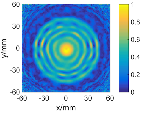
The fields from both the proposed array and the Halbach array (shown in Fig. 4 (a) and Fig. 6 (b) were evaluated by examining the quality of reconstructed images when they are applied as SEM to encode signals of a web-pattern phantom shown in Fig. 7 (a) numerically. The web pattern was used here to clearly show the resolution of the reconstructed image. For encoding, both SEMs were rotated at a step of . Eight surface coils with a diameter of 3 cm were located around the side wall of the cylindrical VoF with a diameter of 20 cm, and used for signal reception. At each angle, 512 readouts were collected for image reconstruction and the SNR of signal was set to be 70 dB. Fig 7 (b), and (c) shows the numerically reconstructed images using the central part () of of the magnetic field from the proposed array (Fig. 4 (a)), and that using the field of the Halbach array (Fig. 6 (b)), respectively. Kaczmarz iteration method was used for the reconstruction. Comparing the images in Fig 7 (b) and (c), clearer features can be seen in the image by using the fields from the proposed array which have an improved monotonicity. The normalized root mean square error (NRMSE) of the image using the proposed array was reduced by about from to compared to that using the reference Halbach array. As can be seen in Fig 7 (b), the blurring, especially at the center of the image is greatly reduced with the proposed array compared to the reference Halbach array. The structural similarity index (SSIM) of the image using the proposed array is 0.446, which is an improvement of about 40% from that using the Halbach array (the SSIM is 0.321). Clearer images can be reconstructed using the magnetic field of the proposed array, which is attributed to the removal of the central zero-gradient region, and that of the regions with low gradients in the field pattern of the proposed array from that of a Halbach array.



4 Discussion
It has been shown that the proposed irregular-shaped ring-pair magnet array provides a monotonic field along a single direction in the central plane of a cylindrical FoV that works for head imaging. Through optimization using GA, the field strength is maintained at above 130 mT with the inhomogeneity controlled at 151840 ppm within the FoV. Due to the linearity in gradient, it serves better as a SEM leading to a better image quality in an MRI system, comparing to a Halbach array [1, 2] and an Aubert-ring-pair aggregate [26]. For a Halbach array with a quadrupolar field pattern, there are regions where the gradients are low or zero, whereas for an Aubert-ring-pair aggregate [26], a gradient in the direction is missing although they can be compensated by adding additional structures or additional mechanical movements of the magnet when conducting encoding. Comparing to an optimized sparse Halbach array [16], the proposed magnet array has a similar length (45.6 cm vs. 45.7 cm in length), but a larger diameter by 21.9 (64 cm vs. 52.5 cm in diameter), and both were designed and optimized to obtain a monotonic SEM for imaging in a FoV with a diameter of 20 cm. The proposed array generates a field with an average field strength of 132.98 mT, which is 64 % higher compared to 81.1 mT of the sparse array. However, the field inhomogeneity of the sparse Halbach array is only about 10 of the proposed array. A large inhomogeneity requires a wider bandwidth of the RF system, which will be discussed in the next paragraph. Overall, the proposed irregular-shaped ring-pair magnet array can be a good candidate to supply the SEM in a low-field portable MRI system, besides a sparse Halbach array [16].
The field homogeneity from the optimized array is decreased from 24786 ppm to 151840 ppm compared to the Aubert-ring-pair aggregate in [26], which can be considered as the price paid for the field monotonicity to favor spatial encoding. The low homogeneity results in the fact that a wide bandwidth are needed for radio-frequency (RF) excitation and signal reception, which may require RF coils and the CONSOLE to have wide working frequency bands. Therefore, as a result, the RF hardware has to be re-engineered to obtain a corresponding broad working bandwidth. Ultra broadband techniques for RF system has been proposed for NMR/MRI systems [35, 36, 19]. A broad-band RF system can by achieved by using, for example, a transformer-based non-resonant transmitter and receiver which covers a broad frequency range [35, 36], or using a receiver with a binary switch array to switch the resonant frequencies spanning in a significantly wide bandwidth [19, 35, 37].
If the requirement for homogeneity can be relaxed further with the implementation of ultra broadband techniques, a more linear field can be obtained from the GA optimization. Fig. 8 shows the field from a design with the relaxed field homogeneity but a much more uniform monotonic gradient pattern compared to the design presented in Section 3. The preset () were the same as those presented in Section 3, and the optimized () were [300 297.6 295.2 292.8 290.4 288.0 285.6 283.2 280.8 278.4 276.0 273.6] (unit: mm). This further optimized design provides a field with an average field strength of 103.04 mT, the field inhomogeneity of 178960 ppm in FoV, and the gradient fields rang from mT to mT along the direction in the region -100 mm50 mm in the central plane (z = 0 mm) of the FoV. Compared to the results presented in Fig. 4, with a compromised field strength and field homogeneity, the monotonic region is wider along the direction and the gradients are close to each other at different values of y. The uniformity of gradients along the direction helps to improve the uniformity of resolution in the reconstructed images [16]. Fig. 7 (d) shows the numerically reconstructed image by using the magnetic field in Fig. 8. In Fig. 7 (d), clearer features are seen at the center of the image with the improved monotonicity compared to Fig. 7 (b). The SSIM of the image using the further improved array is 0.453, which is an increase by 1.5% and 41.1% compared to that using the optimized array and the Halbach one in Fig. 7 (b) and (c), respectively. However, it is worth pointing out that an improved monotonicity is obtained at a price of having a lower field strength and the lower field homogeneity, which may cause a low SNR and a consequent low spatial resolution, and a wide working frequency band for the RF system, respectively.


The FoV is 25 mm off the center of the magnet array to have more regions with monotonic gradients, avoiding the area where the gradient is low (as shown in Fig. 9). The magnet array will be rotated around the center of the FoV rather than the center of the magnet array to facilitate a non-Fourier transform image reconstruction. A rotation mechanism can be designed accordingly to achieve this off-center rotation.


The less number of segments are helpful to reduce the cost of the whole magnet array. Here, the influence of the number of segments on the field pattern was investigated. Each annular magnet under optimization was segmented to 4, 8, 12, 18, 24, and 36 fan-shaped elements, and calculated using (7) and (8), respectively. In all six cases, the were tapered from 300 mm to 273.6 mm (as the design shown in Fig. 8 (b) and (c)) according to the Eq. (9). The field calculated in the central plane (z = 0 mm) of FoV based on different segmentations are shown in Fig. 10 (a-f). The changes of the average field strength and field inhomogeneities (unit: ppm) with the increase of the number of segments were shown in Fig. 10 (g-h). As can be seen, the segmentation with different element numbers showed a similar field pattern and average field strength. However, the field inhomogeneity was influenced a lot by the number of segments as shown in Fig. 10 (h). Overall, will be a suitable range for the number of segments of an annular magnet in the proposed irregular-shaped ring-pair magnet array, which can provide both good field homogeneity and less segments to be calculated.
The fan-shaped magnets are widely used in the designs of motors and in those of accelerators. They are easy to fabricate. However, the optimized magnet array consists of 24 fan-shaped magnets of different dimensions, it would be costly for a physical implementation. The next step for this design is to explore the possibility of using magnet bars and cubes for a similar field pattern with a similar field strength and field homogeneity, probably through optimizing the locations of the magnets.
5 Conclusion
We present a design and the optimization of an irregular-shaped ring-pair magnet array that generates a 1D monotonic field pattern for 2D head imaging. GA was applied for the optimization, and a current model for a fan-shaped ring segment pair was derived for a fast forward calculation for the optimization.In the simulation, the optimized magnet array shows an average field of 132.98 mT and the field homogeneity of 151840 ppm in the a cylindrical FoV with a diameter of 200 mm and a length of 50 mm. Furthermore, the obtained magnetic field was applied as a SEM for signal encoding for imaging for a further evaluation of the proposed magnet array. Kaczmarz iteration method was used for the image reconstructions. The proposed magnet array successfully removes the blur at the central region of the image encoded by a Halbach array due to a highly monotomic gradient. It is a promising alternative to provide SEMs for imaging in a permanent-magnet-based low-field portable MRI system, besides a sparse Halbach array [16] and an Aubert-ring-pair aggregate[26].
References
- [1] Clarissa Zimmerman Cooley, Jason P Stockmann, Brandon D Armstrong, Mathieu Sarracanie, Michael H Lev, Matthew S Rosen, and Lawrence L Wald. Two-dimensional imaging in a lightweight portable mri scanner without gradient coils. Magnetic resonance in medicine, 73(2):872–883, 2015.
- [2] Zhi Hua Ren, Sergei Obruchkov, Dong Wei Lu, Robin Dykstra, and Shao Ying Huang. A low-field portable magnetic resonance imaging system for head imaging. In Progress in Electromagnetics Research Symposium-Fall (PIERS-FALL), 2017, pages 3042–3044. IEEE, 2017.
- [3] Shao Ying Huang, Zhi Hua Ren, Sergei Obruchkov, Jia Gong, Robin Dykstra, and Wenwei Yu. Portable Low-cost MRI System based on Permanent Magnets/Magnet Arrays. arXiv e-prints, page arXiv:1812.10474, December 2018.
- [4] https://www.healthcare.siemens.com/magnetic-resonance-imaging/0-35-to-1-5t-mri-scanner/magnetom-c/features.
- [5] S. M. Wright, D. G. Brown, J. R. Porter, D. C. Spence, E. Esparza, D. C. Cole, and F. R. Huson. The nmr mouse, a mobile universal surface explorer. Magnetic Resonance Materials in Physics, Biology and Medicine, 13:177–18, 2002.
- [6] Juergen Hennig, Anna Masako Welz, Gerrit Schultz, Jan Korvink, Zhenyu Liu, Oliver Speck, and Maxim Zaitsev. Parallel imaging in non-bijective, curvilinear magnetic field gradients: a concept study. Magnetic Resonance Materials in Physics, Biology and Medicine, 21(1-2):5, 2008.
- [7] Gerrit Schultz, Hans Weber, Daniel Gallichan, Walter RT Witschey, Anna M Welz, Chris A Cocosco, Jürgen Hennig, and Maxim Zaitsev. Radial imaging with multipolar magnetic encoding fields. IEEE transactions on medical imaging, 30(12):2134–2145, 2011.
- [8] Jason P Stockmann, Pelin Aksit Ciris, Gigi Galiana, Leo Tam, and R Todd Constable. O-space imaging: highly efficient parallel imaging using second-order nonlinear fields as encoding gradients with no phase encoding. Magnetic resonance in medicine, 64(2):447–456, 2010.
- [9] Jason P Stockmann, Gigi Galiana, Leo Tam, Christoph Juchem, Terence W Nixon, and R Todd Constable. In vivo o-space imaging with a dedicated 12 cm z2 insert coil on a human 3t scanner using phase map calibration. Magnetic resonance in medicine, 69(2):444–455, 2013.
- [10] Klaus Halbach. Strong rare earth cobalt quadrupoles. Nucl. Sci., NS-26:3882––3884, 1979.
- [11] Klaus Halbach. Design of permanent multipole magnets with oriented rare earth cobalt material. Nuclear instruments and methods, 169(1):1–10, 1980.
- [12] H. RAICH and P. BLUMLER. Design and construction of a dipolar halbach array with a homogeneous field from identical bar magnets: Nmr mandhalas. Concepts Magn. Reson, 23B:16–25, 2002.
- [13] Klaas P Pruessmann, Markus Weiger, Markus B Scheidegger, and Peter Boesiger. Sense: sensitivity encoding for fast mri. Magnetic resonance in medicine, 42(5):952–962, 1999.
- [14] Gerrit Schultz, Peter Ullmann, Heinrich Lehr, Anna M Welz, Jürgen Hennig, and Maxim Zaitsev. Reconstruction of mri data encoded with arbitrarily shaped, curvilinear, nonbijective magnetic fields. Magnetic resonance in medicine, 64(5):1390–1403, 2010.
- [15] Gerrit Schultz, Peter Ullmann, Heinrich Lehr, Anna M Welz, Jürgen Hennig, and Maxim Zaitsev. Reconstruction of mri data encoded with arbitrarily shaped, curvilinear, nonbijective magnetic fields. Magnetic resonance in medicine, 64(5):1390–1403, 2010.
- [16] Clarissa Zimmerman Cooley, Melissa W Haskell, Stephen F Cauley, Charlotte Sappo, Cristen D Lapierre, Christopher G Ha, Jason P Stockmann, and Lawrence L Wald. Design of sparse halbach magnet arrays for portable mri using a genetic algorithm. IEEE transactions on magnetics, 54(1):1–12, 2018.
- [17] G Eidmann, R Savelsberg, P Blümler, and B Blümich. The nmr mouse, a mobile universal surface explorer. Journal of Magnetic Resonance, 122:104–109, 1996.
- [18] Bernhard Blumich. NMR imaging of materials, volume 57. OUP Oxford, 2000.
- [19] Pablo J Prado. Single sided imaging sensor. Magnetic resonance imaging, 21(3-4):397–400, 2003.
- [20] J Perlo, F Casanova, and B Blümich. 3d imaging with a single-sided sensor: an open tomograph. Journal of Magnetic Resonance, 166(2):228–235, 2004.
- [21] B Blümich, V Anferov, S Anferova, M Klein, R Fechete, M Adams, and F Casanova. Simple nmr-mouse with a bar magnet. Concepts in Magnetic Resonance: An Educational Journal, 15(4):255–261, 2002.
- [22] Andrew E Marble, Igor V Mastikhin, Bruce G Colpitts, and Bruce J Balcom. A constant gradient unilateral magnet for near-surface mri profiling. Journal of Magnetic Resonance, 183(2):228–234, 2006.
- [23] Wei-Hao Chang, Jyh-Horng Chen, and Lian-Pin Hwang. Single-sided mobile nmr with a halbach magnet. Magnetic resonance imaging, 24(8):1095–1102, 2006.
- [24] Peter BlüMler. Proposal for a permanent magnet system with a constant gradient mechanically adjustable in direction and strength. Concepts in Magnetic Resonance Part B: Magnetic Resonance Engineering, 46(1):41–48, 2016.
- [25] Guy Aubert. Cylindrical permanent magnet with longitudinal induced field, May 7 1991. US Patent 5,014,032.
- [26] Zhi Hua Ren, Wen Chuan Mu, and Shao Ying Huang. Design and optimization of a ring-pair permanent magnet array for head imaging in a low-field portable mri system. IEEE Transactions on Magnetics, 2018.
- [27] A. Trakic, H. Wang, E. Weber, B.K. Li, M. Poole, F. Liu, and S. Crozier. Sense: sensitivity encoding for fast mri. Journal of Magnetic Resonance, 201(2):186––198, 2009.
- [28] Kalyanmoy Deb, Amrit Pratap, Sameer Agarwal, and TAMT Meyarivan. A fast and elitist multiobjective genetic algorithm: Nsga-ii. IEEE transactions on evolutionary computation, 6(2):182–197, 2002.
- [29] Nicholas R Shaw and Richard E Ansorge. Genetic algorithms for mri magnet design. IEEE Transactions on Applied Superconductivity, 12(1):733–736, 2002.
- [30] Yingying Yao, Youtong Fang, Chang Seop Koh, and Guangzheng Ni. A new design method for completely open architecture permanent magnet for mri. IEEE Transactions on Magnetics, 41(5):1504–1507, 2005.
- [31] Edward P Furlani. Permanent magnet and electromechanical devices: materials, analysis, and applications. Academic press, 2001.
- [32] Madabushi VK Chari and P Peter Peet Silvester. Finite elements in electrical and magnetic field problems. John Wiley & Sons Incorporated, 1980.
- [33] Pascal Elleaume, Oleg Chubar, and Joel Chavanne. Computing 3d magnetic fields from insertion devices. In PAC, volume 97, page 3509, 1997.
- [34] Zhi Hua Ren, Luc Maréchal, Wan Luo, Jiasheng Su, and Shao Ying Huang. Magnet array for a portable magnetic resonance imaging system. In RF and Wireless Technologies for Biomedical and Healthcare Applications (IMWS-BIO), 2015 IEEE MTT-S 2015 International Microwave Workshop Series on, pages 92–95. IEEE, 2015.
- [35] D Murphree, SB Cahn, D Rahmlow, and D DeMille. An easily constructed, tuning free, ultra-broadband probe for nmr. Journal of Magnetic Resonance, 188(1):160–167, 2007.
- [36] S Mandal, S Utsuzawa, DG Cory, M Hürlimann, M Poitzsch, and Y-Q Song. An ultra-broadband low-frequency magnetic resonance system. Journal of Magnetic Resonance, 242:113–125, 2014.
- [37] Timothy Hopper, Soumyajit Mandal, David Cory, Martin Hürlimann, and Yi-Qiao Song. Low-frequency nmr with a non-resonant circuit. Journal of Magnetic Resonance, 210(1):69–74, 2011.
Acknowledgements
Z. H. Ren would like to thank the support from the Singapore University of Technology and Design President Graduate Fellowship. This work was supported by Singapore-MIT Alliance for Research and Technology Innovation Grant (ING137068).