Feasibility of single-shot realizations of conditional three-qubit gates in exchange-coupled qubit arrays with local control
Abstract
We investigate the feasibility of single-shot Toffoli- and Fredkin-gate realizations in qubit arrays with Heisenberg-type exchange interactions between adjacent qubits. As follows from the Lie-algebraic criteria of controllability, such an array is rendered completely controllable – equivalent to allowing universal quantum computation – by a Zeeman-like control field with two orthogonal components acting on a single “actuator” qubit. Adopting this local-control setting, we start our analysis with piecewise-constant control fields and determine the global maxima of the relevant figure of merit (target-gate fidelity) by combining the multistart-based clustering algorithm and quasi-Newton type local optimization. We subsequently introduce important practical considerations, such as finite frequency bandwidth of realistic fields and their leakage away from the actuator. We find the shortest times required for high-fidelity Toffoli- and Fredkin-gate realizations and provide comparisons to their respective two-qubit counterparts – controlled-NOT and exponential-SWAP. In particular, the Toffoli-gate time compares much more favorably to that of controlled-NOT than in the standard decomposition-based approach. This study indicates that the use of the single-shot approach can alleviate the burden on control-generating hardware in future experimental realizations of multi-qubit gates.
pacs
03.67.Hk, 03.67.Lx, 75.10.PqI Introduction
Recent years have witnessed rapid progress in the realm of quantum computing (QC), along with the development of methods for coherent control of a broad class of relevant systems QCr. With single-qubit measurement- and control fidelities being already above the fault-tolerance threshold, the attention of workers in the field is now shifting to implementing scalable qubit-array architectures required for fault-tolerant QC rec. Current developments in this direction are an important stride towards the establishment of noisy intermediate-scale quantum technology (systems containing from 50 to a few hundred qubits) Pre in the next few years, a prerequisite for reaching the goal of large-scale universal QC (UQC). In particular, an array of nine spin qubits of Loss-DiVincenzo type Los; Klo – with Heisenberg-type exchange interaction between adjacent qubits – has already been deployed Zaj. Arrays with this type of two-qubit coupling have also been realized in other physical platforms Vel; Ras.
The usefulness of Heisenberg interaction within the circuit model of QC has long been amply appreciated, despite the early realization that this interaction by itself – unlike its lower-symmetry Ising and counterparts – does not allow for UQC DiV. Importantly, it was demonstrated that UQC can still be realized with Heisenberg interaction alone if encoded qubit states are introduced, so that the role of logical qubits is played by triples DiV or pairs Lev of physical qubits. This led to the concept of encoded universality Enc. More recently, another example for the versatility of this type of two-qubit coupling was unravelled through Lie-algebraic studies of spin- systems with time-independent interacting Hamiltonians, which are subject to external time-dependent control fields coupled to certain internal degrees of freedom Sch; Wang et al. 2016. Namely, it was shown that a qubit array with “always-on” Heisenberg interaction is rendered completely controllable provided that at least two noncommuting controls – for example, a Zeeman-type control Hamiltonian that corresponds to a magnetic field with nonzero components in two mutually orthogonal directions (e.g., and ) – act on a single qubit in the array Wang et al. 2016. In other words, an arbitrary quantum gate on any subset of qubits within the given array can then be enacted, which amounts to UQC. Such scenario, with external fields acting on a single qubit in an array, is the extreme version of the local-control approach Heu.
Regardless of the physical realization and its attendant type of two-qubit coupling, one of the central challenges on the way to a large-scale UQC is to reach sufficient accuracy in realizing quantum gates for fault-tolerant QC Pre. A complex quantum circuit – for instance, a multi-qubit gate – can always be decomposed into a sequence of primitive single- and two-qubit gates Nielsen and Chuang 2000. Yet, such an approach is often impractical due to prohibitively long operation times. Besides, the number of gates needed for a quantum algorithm grows rapidly with the system size, with errors being accumulated with each successive gate. One alternative to the established decomposition-based approach entails the use of external control fields to enable fast single-shot realizations of multi-qubit gates. Control-based protocols Gre; Con a have proven to be a viable route to optimized quantum-gate operations Ash in systems ranging from superconducting SCq; Stojanović et al. 2012; Zah to nuclear-spin-based qubit arrays Con c.
This paper investigates the feasibility of single-shot realizations of two conditional three-qubit gates in qubit arrays with Heisenberg interaction. To be more specific, it is focussed on quantum Toffoli and Fredkin gates facilitated by a Zeeman-type local control, this choice of gates being motivated by their importance in quantum information processing Tof. These two gates play key roles in reversible computing, each of them forming a universal gate set together with the (single-qubit) Hadamard gate Nielsen and Chuang 2000. The Toffoli gate is also an important ingredient in quantum error correction (QEC) Ree.
The implementation of the Toffoli gate was already attempted in a variety of QC platforms using the standard decomposition-based approach Mon; Lan; Ree. Yet, all those attempts resulted in sub-threshold fidelities, ranging from in circuit QED to in photonic systems Lan. As regards the Fredkin gate, the progress on the experimental side is even less satisfactory. This gate was demonstrated non-deterministically not so long ago in linear-optics experiments Fred, followed by the realization with a fidelity of around in the context of entangling continuous-variable bosonic modes in three-dimensional circuit QED quite recently Exch.
While a number of proposals for realizing Toffoli and Fredkin gates were put forward in recent years, these gates have never been demonstrated in qubit arrays with Heisenberg-type interaction. The principal rationale for realizing them in a single-shot fashion stems from the fact that, e.g., for spin qubits it has proven challenging to simultaneously achieve fast, high-fidelity single- and two-qubit gates Klo. This state of affairs is the main motivation for the present investigation. While this study is also motivated by the recent physical implementations of Heisenberg-coupled qubit arrays, here we aim for generality and thus opt for an implementation-independent investigation.
The most widely used approaches presently used in high-dimensional optimization problems entail gradient-based greedy algorithms for local optimization, which scale favorably with the problem size NRc. Here we determine the global maxima of the relevant figure of merit (gate fidelity) by combining a greedy quasi-Newton type local-optimization technique and the multistart-based clustering algorithm which facilitates searches for global maxima of objective functions Tor. In this manner, we find both the shortest times required for high-fidelity realizations of the chosen conditional three-qubit gates and the corresponding optimal control fields.
The remainder of this paper is organized as follows. To set the stage, Sec. II recapitulates the main Lie-algebraic results of quantum operator control, introduces the concept of local control and, finally, explains its consequences for qubit arrays with Heisenberg-type interactions. In Sec. III we specify the system under investigation, describe its possible physical realizations, and introduce our control objectives. Sec. IV is set aside for the description of our envisioned control scheme, as well as our procedures for finding optimal piecewise-constant control fields and their spectral filtering. The main findings of the paper are presented and discussed in Sec. V. After an outlook on open-system effects in Sec. VI, we conclude with a brief summary of the paper in Sec. VII.
II Local control in qubit arrays with Heisenberg interaction
II.1 Liealgebraic criteria of controllability
Consider a quantum system with a time-independent drift Hamiltonian , which is acted upon by external control fields () that couple to certain degrees of freedom of the system represented by Hermitian operators . Its total Hamiltonian reads
| (1) |
The dynamical equation for the time-evolution operator of the system, along with its initial condition, has the form characteristic of bilinear control systems (for convenience, hereafter we set ) D’Alessandro 2008:
| (2) |
The goal of a typical quantum-control problem is to find a time and controls such that a desired unitary operation is reached at , i.e., . In particular, the system is completely controllable if its dynamics governed by can give rise – through appropriately chosen fields – to an arbitrary unitary operation on its Hilbert space (), i.e., if the reachable set of the system (the set of unitary operations achievable by varying the controls) coincides with the Lie group or D’Alessandro 2008.
The controllability criteria for quantum systems are formulated using Lie-algebraic concepts Hua, with the dynamical Lie algebra (DLA) of the system playing the central role D’Alessandro 2008. For a system described by the Hamiltonian in Eq. (1), the DLA is generated by the operators , i.e., the skew-Hermitian counterparts of . Importantly, a necessary and sufficient condition for complete controllability is that is isomorphic to or D’Alessandro 2008, the Lie algebras of skew-Hermitian, or traceless skew-Hermitian, matrices Pfeifer 2003. This last result (the Lie-algebraic rank condition) is an existence theorem guaranteeing that any unitary operation on the Hilbert space of the system is reachable by an appropriate choice of control fields. An altogether separate question pertains to finding their actual time dependence that allows one to realize a desired unitary operation, taking into account various practical constraints such as the one on the total duration of the control.
II.2 Local control and its application to qubit arrays
The central control-related question in the context of interacting quantum systems is whether a given system can be partially – in the sense of allowing the realization of specific unitaries – or, perhaps, fully controlled by solely acting on its subsystem. This is the principal idea behind the local-control approach. Namely, even if controls act only on a small subsystem, their effect may be rendered global by the presence of interactions. Needless to say, the choice of the relevant subsystem depends on the type of interaction in the physical system under consideration.
To formalize these last considerations, assume that a composite system is described by a Hamiltonian , where is the coupling (drift) part (acting on the whole ), and are local operators (acting on only); are time-dependent control fields. Assuming, for simplicity, that ’s are generators of the local Lie algebra of skew-Hermitian operators acting on , the system is completely controllable if and only if , are the generators of its corresponding Lie algebra , i.e.,
| (3) |
where is the algebraic closure of the operator sets and Pfeifer 2003. Thus, an arbitrary unitary on can be enacted via a control on its subsystem if and only if all elements of can be obtained as linear combinations of , , and their repeated commutators.
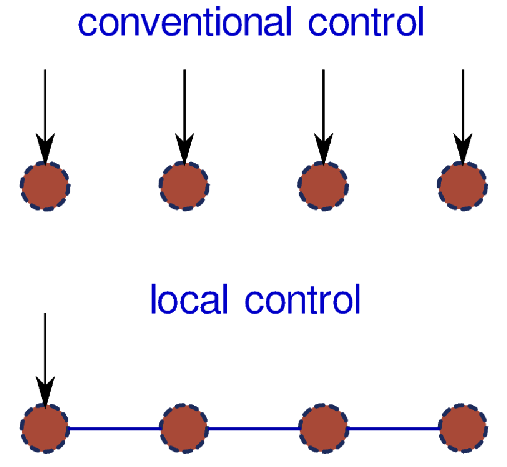
In addition to its conceptual importance, the local-control approach lends itself to applications in qubit arrays Loc, systems that provide a natural setting for UQC. In accordance with the above Lie-algebraic criteria (cf. Sec. II.1), complete controllability of a -qubit array on its -dimensional Hilbert space requires that its attendant DLA be isomorphic with or . Conventional control in an array entails control fields acting on each qubit to enable single-qubit operations (for illustration, see the upper portion of Fig. 1). Combined with a drift Hamiltonian, i.e., two-qubit interactions, this allows in principle the realization of arbitrary (multi-qubit) gates. By contrast, in the local-control approach such fields act only on a small subset of actuator qubits, which in the extreme case can be reduced to a single qubit (the lower part of Fig. 1). The choice of actuators should ideally be one that guarantees complete controllability, as the latter is equivalent to UQC D’Alessandro 2008.
Apart from its simpler implementation, local control is advantageous because reducing the number of controls alleviates the debilitating effects of noise and decoherence (see Sec. VI). While not being the most critical issue in relatively small qubit arrays that are currently being deployed, this will become important already in the near future with the anticipated realization of systems with a few hundred qubits Pre en route to large-scale UQC.
II.3 Controllability of spin- chains (qubit arrays) with Heisenberg-type interactions
The problem of identifying the minimal resources for controllability in interacting spin- systems, i.e., the smallest subsystem that – when acted upon by external control fields – renders the whole system completely controllable, was studied extensively Sch; Wang et al. 2016. Those studies mostly relied upon standard (two-body) interacting spin- models (Ising, , Heisenberg) as their drift Hamiltonians [ in Eq. (1)], with the role of controls [ in Eq. (1)] played by local operators representing individual spins. Because these ingredients coincide with those typically found in qubit arrays, the above control studies have far-reaching implications for the latter.
The most important controllability-related result for our present purposes, derived using a graph-infection criterion, is that the existence of two mutually noncommuting local controls acting on one end spin of a nearest-neighbor -Heisenberg spin- chain ensures complete controllability of the chain Wang et al. 2016. The underlying drift Hamiltonian reads
| (4) |
where is the exchange constant and the anisotropy parameter, while the control Hamiltonian
| (5) |
corresponds to a Zeeman-type control field with nonzero - and components.
The problem of controllability in spin- chains (qubit arrays) with Heisenberg-type interactions has recently been revisited based on a method that makes use of the Hilbert-space decomposition into a tensor product of minimal invariant subspaces Wang et al. 2016. In this manner, it was demonstrated that the last result holds even for the fully anisotropic coupling case, i.e., for the drift Hamiltonian
| (6) |
Moreover, it was shown that the two noncommuting controls need not be applied to one of the end qubits. Finally, the result holds even if the two controls are applied to different – rather than the same – qubits. Needless to say, the described general controllability result applies in the special case of the isotropic Hamiltonian
| (7) |
which is of most relevance for applications in qubit arrays. The last Hamiltonian is the case of Eq. (4), and case of Eq. (6). It will be our working drift Hamiltonian in the following.
For any of the Hamiltonians in Eqs. (4)-(7) and an arbitrary fixed qubit-array size , complete controllability can be demonstrated by showing that the DLA of the system, generated by the set of skew-Hermitian traceless operators (where , or ), has the dimension , with being the dimension of the Hilbert space of the system. This implies that is isomorphic with Pfeifer 2003.
As already mentioned in Sec. II.2, complete controllability amounts to UQC, i.e., it guarantees that an arbitrary gate can be enacted through an appropriate (gate-specific) choice of control fields. It should be stressed that in Heisenberg-coupled qubit arrays a smaller degree of control than that required for UQC can be sufficient for nontrivial computational tasks. Namely, a single local control (e.g., an -only Zeeman-type control on one qubit) is sufficient for controllability of a qubit array on all of its invariant subspaces Wang et al. 2016. The largest among them has the dimension that is exponential in the number of qubits, thus being a useful quantum-computing resource. This reduced degree of control also allows for the realization of nontrivial gates, such as the (the square root of a SWAP gate) – a natural entangling two-qubit gate for exchange-coupled qubits Heu.
For completeness, it is worth mentioning that – by contrast to those of Heisenberg-type – other drift Hamiltonians of interest in realistic qubit arrays do not lead to complete controllability under the same (local-control) circumstances. For a -type Hamiltonian [ case in Eq. (4)], this is intimately related to the fact that the interaction is not algebraically propagating Wang et al. 2016. In the case of Ising coupling controls on each qubit are even required for complete controllability, which amounts to the conventional-control scenario (recall Sec. II.2).
III System and target gates
III.1 Total Hamiltonian and basic assumptions
In what follows, we consider a qubit array with nearest-neighbor Heisenberg coupling, subject to a local control of the first qubit in the array. We express all frequencies and control-field amplitudes in units of the coupling strength (recall that ). Consequently, all the relevant times are expressed in units of .
We take as our point of departure the Hamiltonian , with the drift part given by the isotropic-Heisenberg Hamiltonian of Eq. (7) and the control part by the Zeeman-type Hamiltonian of Eq. (5)
| (8) | |||||
| (9) |
both, for convenience, rewritten in terms of Pauli matrices [ recall that for qubit ]. We will also consider the effects of a static global magnetic field in the direction, a situation captured by the drift Hamiltonian
| (10) | |||||
where quantifies the magnetic-field strength.
Realistic control fields – e.g., magnetic fields realized using micromagnets Pio – are never perfectly localized. Thus, our original assumption about the control being confined to a single qubit in an array is, strictly speaking, an idealization. A more realistic scenario entails a field that also affects neighboring qubits due to field leakage, a situation that requires a slight generalization of the Hamiltonian in Eq. (9). Assuming an exponential field decay away from the first qubit, the relevant control Hamiltonian adopts the form Wang et al. 2016
| (11) |
where the parameter measures the extent of control-field leakage.
It is worth pointing out that the field-leakage effect does not invalidate the rationale for using the local-control approach. Namely, in Ref. Wang et al. 2016 it was demonstrated that the subspace-controllability results are robust with respect to leakage, in that the invariant-subspace structure and controllability of the system remain unchanged. By extension these results imply that the conclusions about complete controllability remain valid in the presence of such leakage.
It is pertinent to stress that – as most gate-optimization treatments – the present work corresponds to the closed-system scenario, i.e., to the unitary dynamics of the system within the open-loop coherent control framework. In other words, the unavoidable debilitating effects of decoherence due to an interaction of qubits with the environment (open-system scenario) are not explicitly taken into account. The most general analysis of the gate-optimization problem would, however, require one to incorporate an interaction of qubits with a multi-mode bosonic bath, as briefly discussed in Sec. VI.
III.2 Physical realizations
Qubit arrays with nearest-neighbor isotropic Heisenberg exchange interactions can be realized using different physical platforms. While this type of interaction is a natural physical ingredient in the case of spin qubits Klo, it is worthwhile to elaborate on how it can even be realized with superconducting (SC) systems, in which the most commonly occurring coupling between qubits is of type Wen. [Note that in the condensed-matter physics terminology the latter is referred to as coupling.] SC systems, in fact, allow one to realize a more general class of Hamiltonians than the one in Eq. (7) – namely, those of the Heisenberg type [cf. Eq. (4)]. Here we describe two approaches to achieve that.
One approach is based on the observation that one-dimensional arrays of capacitively-coupled SC islands can effectively be described as spin- chains Faz. Generally speaking, the part of their effective Hamiltonian features nearest-neighbor two-body interactions, while its part also comprises contributions beyond nearest neighbors. Yet, through an appropriate choice of the junction capacitances, as well as the capacitances of SC islands to the back gate of the structure, the part can effectively be reduced to nearest-neighbor interactions. The Josephson energy of the junctions that couple different islands plays the role of the exchange coupling constant and can be varied using a magnetic field provided that those junctions have the form of a dc-SQUID. The anisotropy parameter corresponds here to the ratio , where is the charging energy. Thus, its different values can be realized by varying this ratio (in particular, is the isotropic-Heisenberg-interaction case). One SC island in the array should be a qubit playing the role of an actuator, while the control fields and are determined by the Josephson energy of this qubit (an additional constant field would correspond to the gate voltage).
Another approach for realizing spin- chains with SC qubits was quite recently laid out in Ref. Ras. This scheme makes use of a complex SC circuit based on an array of qubits mutually connected through coupler circuits. The latter either contain a Josephson junction (or a dc-SQUID) in parallel with an inductor, or – for every other such coupler – these two elements connected in parallel with an additional capacitor. While several other types of SC qubits (transmon, X-mon, fluxonium, etc.) could in principle be utilized in this envisioned system, it turns out that the most realistic parameters are obtained for capacitively-shunted flux qubits Wen.
In state-of-the-art solid-state QC setups in the microwave regime (based on SC- or spin qubits) Rei; vdi, precisely-shaped control pulses are obtained using arbitrary waveform generators (AWGs), currently available with sub-nanosecond time resolution. To be more precise, in the conventional approach for control-pulse synthesis AWGs only generate a baseband signal and a desired pulse is then obtained through an upconversion to microwave frequencies by mixing with a carrier. However, the continuously improving sampling rates of AWGs – currently approaching gigasamples per second – now allow direct digital synthesis of microwave pulses Rya, thus obviating the need for separate microwave generators. Thus, these high-bandwidth AWGs both allow more advanced pulse shaping and reduce the number of hardware components in QC setups.
III.3 Control objectives (target gates)
Our objective is to realize Toffoli and Fredkin gates in an array with qubits with the first qubit playing the role of actuator. The same qubit will also be the control qubit in the Fredkin-gate realizations, while in the context of the Toffoli gate it will also be one of the control qubits. At the same time, the third qubit will play the role of the target qubit for both gates.
A Toffoli (controlled-controlled-NOT) gate enacts a Pauli- (flip) operation on the third (target) qubit if the first two (control) qubits are both set (i.e., both are in the state), doing nothing otherwise Nielsen and Chuang 2000,. It represents a generalization of controlled-NOT (CNOT), an entangling two-qubit gate. Arguably the most important application of the Toffoli gate is in the measurement-free QEC Ree, where it effectively replaces the measurement- and correction steps of the standard QEC.
A Fredkin (controlled-SWAP) gate enacts a SWAP operation between the second and third qubits, if the first (ancilla) qubit is set, otherwise leaving their states unchanged Nielsen and Chuang 2000. In other words, it enacts an entangling operation between those two qubits by performing a superposition of the identity and SWAP gates. While this operation is conditioned on the state of the ancilla qubit, thus giving rise to tripartite entanglement, its closest two-qubit counterpart is exponential-SWAP (eSWAP) – an unconditional entangling operation given by .
Toffoli and Fredkin gates are self-inverse operations (), i.e., two consecutive applications of these gates amount to the identity operation (). This fact has profound consequences for the shape of the optimal control-pulse sequences (see Sec. V.1).
IV Methodology
IV.1 Control scheme and its justification
Our goal is to find the time dependence of control fields and for high-fidelity realizations of the desired three-qubit gates in a system with qubits. For the sake of simplicity, we will attempt to synthesize the corresponding optimal-field waveforms starting from piecewise-constant (hereafter abbreviated as PWC) control fields applied in alternation in the and directions with the respective amplitudes and (). In the following, we describe our envisioned control scheme, which represents one special realization of the control Hamiltonian in Eq. (9).
At a pulse is applied in the direction with the constant amplitude during the time interval . The corresponding Hamiltonian of the system during this interval is given by . Then a pulse with the amplitude is applied during the interval , whereby the system dynamics are governed by the Hamiltonian . This sequence of alternating and pulses is continued until pulses have been carried out by the time . The resulting time-evolution operator of the system is obtained by concatenating operators and for :
| (12) |
Our chosen local-control scheme is based on a successive switching between - and -control Hamiltonians ( and , respectively). It represents a slight generalization of a well-known switching scheme that was proven by Lloyd to be sufficient for UQC Lloyd 1995. Namely, if and are Hermitian matrices of dimension and the Lie algebra they generate through commutation, then for any the unitary matrix can be expressed in the form with finite . This last result, which was put on a rigorous mathematical footing in Ref. Wea, can be viewed as a consequence of an even more general result pertaining to uniform finite generation of connected compact Lie groups [such as or ] D’Alessandro 2008. That result asserts that for a connected Lie group corresponding to a Lie algebra , every element can be expressed through a finite number of factors of the type , where is one of the generators of and .
The crucial implication of the above mathematical results for the system at hand is that an arbitrary unitary operation acting on its Hilbert space – including our target conditional three-qubit gates – can be obtained with a finite sequence of operators and . For the sake of simplicity, our elected control schemes assumes that all time slices have equal length, i.e., that for each .
IV.2 Numerical optimization of target-gate fidelities
The problem at hand represents a unitary gate synthesis up to a global phase in a closed quantum system. Therefore, we will make use of the standard figure of merit for this subclass of problems in quantum operator control – the (normalized) phase invariant distance to the target unitary (here a three-qubit quantum gate) at the final time – i.e., the trace fidelity
| (13) |
Needless to say, in accordance with the comments made at the end of Sec. III.1, the last expression and all the results to be presented below correspond to the intrinsic fidelity (fidelity in the absence of decoherence).
For each target gate, we maximize its fidelity – equivalent to minimizing the gate error – over the control amplitudes , () for varying total number () and duration () of pulses (time slices). Finding the global maximum of constitutes a nontrivial numerical-optimization problem. We perform this complex task using the multistart-based clustering algorithm which entails the following steps Tor. One starts from a large sample of random points in the space of candidate solutions (set of control amplitudes). One then selects a smaller number of them that yield the largest fidelities and performs local searches for maxima around each of these points: the one with the highest value of the fidelity is then adopted as the sought-after global maximum. The validity of this approach is corroborated by the stability of the final result for the global maximum upon varying the initial number of random points.
Local searches for the maxima of the target-gate fidelity [Eq. (13)] are performed using a second-order concurrent-update method of the quasi-Newton type NRc. The latter requires one to start from an initial guess for the values of the relevant variables (here control-field amplitudes) and an initial Hessian approximation (here taken to be the identity). The control amplitudes are then iteratively updated according to the Newton update rule, while the approximate Hessian is constructed from the past gradient history according to the Broyden-Fletcher-Goldfarb-Shanno (BFGS) formula NRc. After each iteration the objective function [here ] increases, with termination when the desired accuracy is reached. This procedure guarantees convergence to a local maximum of the objective function.
IV.3 Spectral filtering of optimal PWC control fields
While being a conventional starting point in gate optimizations, PWC control fields – which have infinite spectral bandwidths – represent a mathematical idealization. In realistic implementations of quantum control, achievable fields have nonzero Fourier components only in a finite frequency range. Thus, in order to make contact with experiments it is necessary to perform spectral filtering of optimal PWC control fields. In particular, low-pass filters are inherent to all present-day AWGs.
Constraints on the frequency spectra of the control fields () are imposed through filter functions. The filtered fields are obtained by first operating with a filter function on the Fourier transforms of the optimal fields, and then switching back to the time domain via inverse transform
| (14) |
In particular, we will make use of an ideal low-pass filter which removes the Fourier components at frequencies outside the interval , i.e., . Using the general expression in Eq. (14), in this special case we obtain Heu
| (15) |
where and . The time-evolution operator corresponding to the filtered fields – from which the attendant gate fidelities are easily obtained using the expression in Eq. (13) – can be computed using an unconditionally stable numerical method based on a product-formula approximation Heu.
Therefore, experimentally-feasible (finite-bandwidth) control fields are here obtained through post-processing, i.e., low-pass filtering, of their optimized PWC counterparts. In connection with our use of this approach, the following two remarks are in order here.
While PWC control fields successively applied in the - and directions represent our point of departure in the present work (cf. Sec. IV.1), the filtered fields and generically both have nonzero values throughout the interval . Thus, our inherently simple control scheme does not bear a significant loss of generality compared to the more general control protocol in which the initial PWC control fields simultaneously have nonzero components in both relevant spatial directions.
For completeness, it is worthwhile to note that an alternative approach to obtaining finite-bandwidth control fields would entail imposing a spectral-bandwidth constraint from the outset, i.e., incorporating it a priori in the numerical search for optimal control fields. Such an approach has quite recently been demonstrated by Lucarelli Luc. That approach – computationally much more demanding than the one utilized here – relies on the use of Slepian sequences, finite-length sequences that represent the space of band-limited signals and serve as the basis functions for PWC control fields.
V Results and Discussion
In what follows, we present our findings, starting from the results obtained for the Toffoli- and Fredkin gate fidelities in the idealized situation where PWC control fields act on a single actuator qubit. We then discuss a more realistic setting that entails filtered control fields or their leakage away from the actuator. Finally, we also discuss the effect that the presence of a static global magnetic field has on the gate fidelities and gate times. To illustrate the efficiency of our approach, we also provide comparisons of the Toffoli- and Fredkin gate times with the gate times corresponding to their respective two-qubit counterparts – CNOT and eSWAP.
As our target intrinsic gate fidelity for PWC control fields we adopt (i.e., ), which was once widely accepted as the threshold for fault-tolerant QC Ste; Kni. It is worth mentioning, however, that QC schemes with significantly lower thresholds – with gate errors as high as – have been proposed more recently Hig. Bearing this is mind, we adopt and as our target gate errors – corresponding to the target intrinsic gate fidelities of and , respectively – in the more realistic setting described above.
V.1 Optimal PWC and filtered control fields
Our optimization of the gate fidelities shows two central features. Firstly, for a fixed total time the gate fidelities depend significantly on the total number of pulses; they increase upon increasing (or, equivalently, decreasing the duration of a single pulse). Secondly, each gate has its own characteristic shortest gate time required to reach a fidelity close to unity, below which such fidelities are unreachable regardless of .
In particular, we find that the shortest Toffoli-gate time required to reach an intrinsic fidelity within our approach is approximately . The corresponding optimal - and PWC control fields, corresponding to pulses, are depicted in Fig. 2. The shortest times required to realize the same gate with somewhat larger gate errors of and are approximately and , respectively.


It is instructive to compare the obtained Toffoli-gate times with those of CNOT, its two-qubit counterpart. For instance, the shortest times needed to realize CNOT on the second- and third qubit in the same system with the respective fidelities of and (i.e.,the gate errors of and ) we find to be approximately and . Therefore, the shortest Toffoli-gate time within our single-shot approach compares much more favorably to that of CNOT than is the case within the standard decomposition-based approach, where the optimal CNOT-gate cost of a Toffoli gate is 6 She. In previous studies of single-shot gate realization, favorable comparisons of Toffoli- and CNOT gate times were found only in some special cases Ash. Thus, the results obtained here can be attributed to the versatility of the exchange interaction and our adopted control scenario.
As regards the Fredkin gate, the shortest time required to realize it with an intrinsic fidelity is approximately , while the respective times needed to realize this gate with the errors of and are approximately and . The optimal pulse sequence corresponding to , with the total of pulses, is depicted in Fig. 3 and has the interesting property of being palindromic in nature.
It is worth pointing out that palindromic pulse sequences are a common occurrence for self-inverse gates (͑cf. Sec. III.3) and result from specific properties of underlying Hamiltonians under the time-reversal transformation (, ). Because the Toffoli gate is a self-inverse operation too, a palindromic optimal pulse sequence could have, in principle, also been expected for this gate. Yet, our numerical-optimization procedure apparently yields another pulse sequence that corresponds to a higher fidelity.
By analogy to the previously made comparison between the Toffoli and CNOT-gate times, it is judicious to compare the obtained Fredkin-gate times with those corresponding to the closely related two-qubit gate – eSWAP (recall Sec. III.3). Our numerical computation shows that the shortest times required to realize the eSWAP gates corresponding to , and with an intrinsic fidelity of are all aproximately equal to . For the eSWAP-gate times needed to reach an intrinsic fidelity of we obtain for and , while for we get . Finally, those that correspond to are approximately for , for , and for . Thus the obtained Fredkin-gate times are just slightly longer than those characteristic of eSWAP, which is another sign of the effectiveness of our approach.
The quantitative effect of spectral low-pass filtering of the obtained optimal PWC control fields on the Toffoli- and Fredkin-gate fidelities is illustrated in Figs. 4 and 5, respectively, where the gate error corresponding to the low-pass filtered control fields is shown. What can be inferred from these plots is that fidelities as high as can be preserved for the cut-off frequencies (Toffoli gate) and (Fredkin gate).


It is worthwhile to stress that for a typical range of magnitudes of exchange-coupling constants in spin- and SC-qubit systems ( MHz), the obtained cut-off frequencies are well within the range achievable with state-of-the-art AWGs Stojanović et al. 2012. Thus, low-pass filtering (recall Sec. IV.3) – which turns infinite-bandwidth optimal PWC control fields into realistic finite-bandwidth ones – does not present an obstacle to achieving high gate fidelities within our present approach.
V.2 Effects of control-field leakage
The effect of control-field leakage – as quantified by the parameter – on the fidelities of the Toffoli and Fredkin gates is illustrated in Figs. 6 and 7, respectively. These results make it possible to draw conclusions about the permissible extent of leakage that allows the preservation of high gate fidelities. For the Toffoli gate, our calculations show that in order to retain fidelities above () for the control-pulse sequences optimized for the leakage-free case one needs (), implying that the magnitude of stray fields on the nearest neighbor of the actuator qubit does not exceed () of the original field. Similarly, in the case of the Fredkin gate for preserving such fidelities one needs (). The corresponding magnitude of stray fields on the qubit adjacent to the actuator does not exceed () of the original field.


The obtained results for the critical extent of leakage that allows high-fidelity realization of the chosen gates should, however, not be taken as a sign that the proposed single-shot approach is highly sensitive to the leakage effects. Namely, the curves in Figs. 6 and 7 show the obtained results for the gate fidelities in the presence of leakage, but those results correspond to the control-pulse sequences optimized for the leakage-free case, where the relevant control Hamiltonian is the one given by Eq. (9). Therefore, they should merely be viewed as benchmark curves, to be used for extracting the actual (system- and gate-specific) value of the leakage parameter . This can be done by comparing the relevant benchmark curve with the fidelity obtained by experimentally running the relevant optimal pulse sequence.
The in-situ leakage-parameter retrieval of the kind described above should be viewed as the first step in any realistic application of the single-shot approach in the local-control setting. Its second step should entail finding another pulse sequence, this time optimized in the presence of leakage, i.e., assuming that the system dynamics are governed by the control Hamiltonian given by Eq. (11), with the previously extracted value of the leakage parameter. This optimization can be carried out using the same approach as in the absence of leakage (cf. Sec. IV.2). As our explicit numerical calculations demonstrate, very high fidelities are achievable even for those values of whose corresponding fidelities in the two benchmark curves significantly deviate from unity. Interestingly, the corresponding gate times are similar to, and in some cases even shorter, than their counterparts in the leakage-free case.
For instance, in the case of the Toffoli-gate realization with , where the corresponding fidelity in the benchmark curve (Fig. 6) is rather low, more precisely slightly below , our calculation shows that the fidelity of can be obtained within approximately . This is actually a shorter gate time than that required for the same fidelity in the leakage-free case (). Similarly, in the Fredkin-gate realization with , where the relevant fidelity in the curve of Fig. 7 is around , a fidelity as high as can be obtained with the gate time of approximately , significantly shorter than in the absence of leakage. These results clearly indicate that our proposed two-step procedure constitutes an efficient scheme for achieving high gate fidelities even in the presence of a substantial control-field leakage away from the actuator qubit. While it was already stated that the presence of leakage does not invalidate the theoretical (Lie-algebraic) basis for the local-control approach (recall the discussion in Sec. III.1), our numerical findings strongly suggest that it also does not diminish the potential practical effectiveness of this approach.
V.3 Effects of a global magnetic field
In addition to the results obtained in the case of the isotropic-Heisenberg drift Hamiltonian of Eq. (8), it is of interest to also analyze the effect that the presence of a residual global magnetic field has on the gate fidelities and the corresponding gate times. This situation is described by the extended drift Hamiltonian of Eq. (10), where the strength of a static Zeeman-type magnetic field in the direction is parameterized by . The numerical procedure utilized to optimize the gate fidelities over control-field amplitudes is exactly the same as in the field-free case (cf. Sec. IV.2).
| Toffoli-gate time | Fredkin-gate time | |||
|---|---|---|---|---|
| 0 | 21 | 25 | 24 | 28 |
| 0.1 | 21 | 29 | 24 | 33 |
| 0.2 | 21 | 27 | 25 | 34 |
| 0.3 | 18 | 25 | 20 | 29 |
| 0.4 | 22 | 25 | 26 | 29 |
| 0.5 | 21 | 26 | 24 | 25 |
| 0.6 | 19 | 27 | 19 | 30 |
| 0.7 | 19 | 28 | 20 | 29 |
| 0.8 | 22 | 28 | 24 | 36 |
| 0.9 | 21 | 22 | 23 | 36 |
| 1.0 | 19 | 30 | 19 | 31 |
| 1.1 | 20 | 25 | 20 | 30 |
| 1.5 | 18 | 27 | 23 | 29 |
The approximate Toffoli- and Fredkin-gate times corresponding to the target intrinsic fidelities of and , obtained for a wide range of values for , are summarized in Table 1. For both three-qubit gates under consideration and both stated target values of the corresponding fidelities, the obtained gate times show an apparent nonmonotonic behavior with increasing and do not deviate significantly from their counterparts found in the absence of the external field. Interestingly, for the target fidelity of , the shortest Toffoli- and Fredkin gate times are quite similar and obtained for the same values of (). This is no longer the case for the higher target fidelity of , where the shortest obtained times for the Toffoli and Fredkin gates correspond to different (non-zero) field strengths.
V.4 Comparison to other approaches for realizing conditional gates
It is instructive to compare the present approach to realizing the Toffoli and Fredkin gates in Heisenberg-coupled qubit arrays to some recent related works.
An efficient scheme has recently been proposed for realizing these conditional three-qubit gates in a SC circuit that comprises two qubits and one qutrit (a three-level generalization of a qubit) and effectively represents an Heisenberg chain Aar. That scheme is, in fact, more general and apart from those two gates can implement in principle any controlled-controlled unitary operation. The latter are exemplified by the double-controlled holonomic single-qubit gate, based on the idea of holonomic quantum computation Zan – a general framework for building universal sets of robust gates using non-Abelian geometric phases. While holonomic gates were originally envisioned to be adiabatic, the scheme in Ref. Aar implements them in a non-adiabatic fashion Sjo.
One obvious common denominator of the present work, based on the optimal-control theory, and the scheme proposed in Ref. Aar is their increased robustness to noise compared to the conventional control protocols. While here this robustness stems from the reduced number of actuator qubits (local control), in the latter scheme it originates from the geometric character of holonomic gates. In particular, nonadiabatic implementations Fen; Che of holonomic gates generally lead to shortened gate times and thereby alleviate the loss of coherence (due to exposure to open-system effects) that typically hampers their adiabatic counterparts. The same effect that can also be achieved using an approach that became known as the shortcut to adiabaticity Che; Iba; Zha.
Generally speaking, it is conceivable that the approaches based on optimal-control theory and shortcuts to adiabaticity can even be combined into a unified framework. This boils down to the fundamental open question as to whether it is possible to connect the Lewis-Riesenfeld invariants Che – used for shortcuts to adiabaticity – with the Pontryagin maximum principle Pon that forms the basis of optimal-control theory. If such a connection proves to be viable, this would allow one to combine the advantages of both approaches.
VI Outlook: open-system effects
As hinted in Sec. III.1 an all-encompassing approach to the gate-optimization problem at hand necessitates the inclusion of open-system effects, i.e., the unavoidable decoherence-induced noise. Here we provide a general assessment of this problem and briefly explain one possible approach for its quantitative treatment.
Regardless of the specific character of the qubit array and its environment (Markovian or non-Markovian), optimal-control-based gate synthesis with the inclusion of open-system effects is, generally speaking, computationally very expensive. This stems from the need to simulate quantum dynamics in a high-dimensional Hilbert space Gra; Flo. For instance, in Ref. Flo such a study was carried out for small qubit systems with Heisenberg-type exchange coupling, which interact with either Markovian or non-Markovian environments. This study concluded that control fields optimized in the absence of the environment (closed system) remain the optimal ones in the Markovian case provided that the decoherence is sufficiently uniform and weak to be viewed as a perturbation of the unitary evolution. On the other hand, such pre-optimized fields were found to perform poorly in the non-Markovian case, thus underscoring the importance of an accurate characterization of the system-environment coupling for high-fidelity gate realizations.
While a full-fledged gate optimization in the open-system scenario is a rather difficult problem, a somewhat simpler task is to quantify how a gate-specific pulse sequence optimized for a closed system performs in the presence of decoherence-induced noise. This naturally entails the notion of the average state fidelity, which for a generic -qubit system is defined as
| (16) |
Here () are the (normalized) computational basis states of the system, while is the density matrix at the end of a nonunitary evolution (i.e., at , where is the time required for a high-fidelity realization of the concrete gate) that starts with the system in the pure state . In other words, , where is the density matrix of the system which satisfies the initial condition . In the framework of the quantum operation formalism Nielsen and Chuang 2000, this density matrix can be written in the form of a sum over (time-dependent) Kraus matrices of the system Kra.
The Kraus matrices of a qubit array are given by the tensor products of those representing individual qubits. To construct these single-qubit matrices one ought to adopt a specific model for the decoherence-induced noise. In one of the widely used models Liu, a qubit is represented by the lowest two number states of a linear harmonic oscillator and the environment as a collection of multimode oscillators. A qubit is subject to two noise processes, namely the amplitude and phase damping, each characterized by its own damping rate – the respective inverses of the amplitude-relaxation- () and dephasing () times. The latter, usually similar in magnitude, are often assumed to be approximately the same and represented by the unique coherence time .
On quite general grounds, assuming that the decoherence-induced errors are mutually independent, the average state fidelity can be expected to be approximately given by , where is the intrinsic fidelity. In cases where the achievable gate times are much shorter than the coherence time (), the last expression simplifies to . Unsurprisingly, such linear dependence of on was predicted, for example, in a theoretical proposal for an avoided-crossing-based Toffoli and Fredkin gates in a system of three coupled SC transmon qubits Zah.
As far as the system at hand is concerned, the characteristic times that we obtained for high-fidelity realizations of Toffoli and Fredkin gates are at most around . For typical magnitudes of exchange-coupling constants in state-of-the-art SC- and spin-qubit systems (cf. Sec. V.1) this amounts to the approximate gate times ns. On the other hand, typical coherence times in both of these classes of solid-state QC platforms are nowadays of the order of several tens-of-microseconds. Therefore, the condition is fulfilled in physical systems of relevance for the present investigation. In accordance with the reasoning mentioned above, this last conclusion also implies that one can expect to extract the linear dependence of on in future studies that will take into account the open-system effects.
VII Summary and Conclusions
To summarize, we investigated the feasibility of single-shot realizations of the Toffoli and Fredkin gates in qubit arrays with Heisenberg-type coupling between adjacent qubits. In doing so, we fully exploited the local controllability of this system, i.e., the fact that it is rendered completely controllable via a Zeeman-like control of a single actuator qubit. This control setting does not only reduce the burden of finding the optimal control fields – by lowering their number – but is also desirable because it alleviates the debilitating effects of decoherence. The present study incorporated two important practical issues of relevance for gate realizations: a finite-frequency range of realistic control fields and their leakage away from the actuator. It was demonstrated that none of these two ingredients presents an obstacle to realizing the Toffoli- and Fredkin gates with high fidelities required for fault-tolerant quantum computing.
The synthesis of complex multi-qubit gates from single- and two-qubit building blocks proved to be quite cumbersome. For example, four-qubit Toffoli gate employed in a recent implementation of Grover’s search algorithm with trapped-ion qubits Fig required as many as two-qubit gates and single-qubit gates. This fuels the need for alternative gate-synthesis approaches that avoid the use of such decompositions Groenland and Schoutens 2018. The present work constitutes an attempt in this direction, specifically devoted to systems with Heisenberg-type exchange interaction between adjacent qubits. In particular, our findings regarding the efficient single-shot realization of the three-qubit Toffoli gate may facilitate future applications of this gate in measurement-free quantum error correction in this type of systems Tan; Soh Likewise, the proposed single-shot Fredkin gate may prove beneficial in the context of recently investigated universal quantum computation utilizing continuous-variable bosonic cavity modes in three-dimensional circuit-QED architecture, where the central physical mechanism behind entangling such modes is an engineered exchange interaction Exch.
In conclusion, fast and accurate realizations of quantum gates remain one of the crucial ingredients towards attaining the overarching goal of universal quantum computation Pre. The present work, which can be generalized to more complex (e.g., higher-dimensional) qubit networks Are, seems to indicate that the use of the single-shot approach could significantly alleviate the burden on control-generating hardware in future experimental realizations of multi-qubit gates. It will hopefully foster further experimental applications of this methodology.
Acknowledgements.
The author acknowledges useful discussions during previous collaborations on related topics with R. Heule, D. Burgarth, C. Bruder, and T. Tanamoto.References
- (1) See, e.g., C. Monroe and J. Kim, Science , 1164 (2013); M. H. Devoret and R. J. Schoelkopf, ibid. , 1169 (2013); D. D. Awschalom, L. C. Bassett, A. S. Dzurak, E. L. Hu, and J. R. Petta, ibid. , 1174 (2013).
- (2) R. Barends et al., Nature (London) 508, 500 (2014); T. F. Watson et al., ibid. 555, 633 (2018).
- (3) J. Preskill, Quantum 2, 79 (2018).
- (4) D. Loss and D. P. DiVincenzo, Phys. Rev. A 57, 120 (1998).
- (5) For a review, see C. Kloeffel and D. Loss, Annu. Rev. Condens. Matter Phys. 4, 51 (2013); R. Hanson, L. P. Kouwenhoven, J. R. Petta, S. Tarucha, and L. M. K. Vandersypen, Rev. Mod. Phys. 79, 1217 (2007).
- (6) D. M. Zajac, T. M. Hazard, X. Mi, E. Nielsen, and J. R. Petta, Phys. Rev. Applied , 054013 (2016).
- (7) M. Veldhorst et al., Nature (London) , 410 (2015).
- (8) S. E. Rassmussen, K. S. Christensen, and N. T. Zinner, arXiv:1808.09881.
- (9) D. P. DiVincenzo, D. Bacon, J. Kempe, G. Burkard, and K. B. Whaley, Nature (London) 408, 339 (2000).
- (10) J. Levy, Phys. Rev. Lett. 89, 147902 (2002).
- (11) D. Bacon, J. Kempe, D. A. Lidar, and K. B. Whaley, Phys. Rev. Lett. 85, 1758 (2000).
- (12) S. G. Schirmer, I. C. H. Pullen, and P. J. Pemberton-Ross, Phys. Rev. A , 062339 (2008).
- Wang et al. (2016) X. Wang, D. Burgarth, and S. G. Schirmer, Phys. Rev. A 94, 052319 (2016).
- (14) R. Heule, C. Bruder, D. Burgarth, and V. M. Stojanović, Phys. Rev. A , 052333 (2010); Eur. Phys. J. D , 41 (2011).
- Nielsen and Chuang (2000) M. A. Nielsen and I. L. Chuang, Quantum Computation and Quantum Information (Cambridge University Press, Cambridge, 2000).
- (16) T. J. Green, J. Sastrawan, H. Uys, and M. J. Biercuk, New J. Phys. 15, 095004 (2013).
- Con (a) For a comprehensive review, see S. J. Glaser et al., Eur. Phys. J. D , 279 (2015).
- (18) S. Ashhab, P. C. DeGroot, and F. Nori, Phys. Rev. A , 052327 (2012).
- (19) See, e.g., S. Montangero, T. Calarco, and R. Fazio, Phys. Rev. Lett. , 170501 (2007); P. Rebentrost and F. K. Wilhelm, Phys. Rev. B , 060507(R) (2009); M. Goerz, D. Reich, and C. Koch, New J. Phys. , 055012 (2014); A. W. Cross and J. M. Gambetta, Phys. Rev. A , 032325 (2015); E. Barnes, C. Arenz, A. Pitchford, and S. E. Economou, Phys. Rev. B , 024504 (2017).
- Stojanović et al. (2012) V. M. Stojanović, A. Fedorov, A. Wallraff, and C. Bruder, Phys. Rev. B 85, 054504 (2012).
- (21) E. Zahedinejad, J. Ghosh, and B. C. Sanders, Phys. Rev. Lett. , 200502 (2015); Phys. Rev. Applied , 054005 (2016).
- Con (c) C. D. Aiello and P. Cappellaro, Phys. Rev. A , 042340 (2015); J. Zhang, D. Burgarth, R. Laflamme, and D. Suter, ibid. , 012330 (2015).
- (23) For recent examples, see J. K. Moqadam, G. S. Welter, and P. A. A. Esquef, Quantum Inf. Process. , 4501 (2016); A. Daskin and S. Kais, ibid. , 33 (2017); F. Holik, G. Sergioli, H. Freytes, R. Giuntini, and A. Plastino, ibid. , 1573 (2017); A. Devra, P. Prabhu, H. Singh, Arvind, and K. Dorai, ibid. , 67 (2018).
- (24) T. Monz et al., Phys. Rev. Lett. , 040501 (2009).
- (25) B. P. Lanyon et al., Nat. Phys. , 134 (2009).
- (26) M. D. Reed, L. DiCarlo, S. E. Nigg, L. Sun, L. Frunzio, S. M. Girvin, and R. J. Schoelkopf, Nature (London) , 382 (2012).
- (27) R. B. Patel, J. Ho, F. Ferreyrol, T. C. Ralph, and G. J. Pryde, Sci. Adv. , e1501531 (2016); T. Ono, R. Okamoto, M. Tanida, H. F. Hofmann, and S. Takeuchi, Sci. Rep. , 45353 (2017).
- (28) Y. Y. Gao, B. J. Lester, K. Chou, L. Frunzio, M. H. Devoret, L. Jiang, S. M. Girvin, and R. J. Schoelkopf, arXiv:1806.07401.
- (29) W. H. Press, S. A. Teukolsky, W. T. Vetterling, and B. P. Flannery, Numerical Recipes in C: The Art of Scientific Computing (Cambridge University Press, Cambridge, 1999).
- (30) A. Törn and A. Žilinskas, Global Optimization, Lecture Notes in Computer Science, vol 350 (Springer, Berlin, 1989).
- (31) V. Jurdjević and H. J. Sussmann, J. Differ. Equations , 313 (1972); G. M. Huang, T. J. Tarn, and J. W. Clark, J. Math. Phys. , 2608 (1983); V. Ramakrishna and H. Rabitz, Phys. Rev. A , 1715 (1996).
- D’Alessandro (2008) D. D’Alessandro, Introduction to Quantum Control and Dynamics (Taylor & Francis, Boca Raton, 2008).
- Pfeifer (2003) W. Pfeifer, The Lie Algebras : An Introduction (Birkhäuser, Basel, 2003).
- (34) See, e.g., S. Lorenzo, T. J. G. Apollaro, A. Sindona, and F. Plastina, Phys. Rev. A , 042313 (2013).
- (35) M. Pioro-Ladriere, T. Obata, Y. Tokura, Y.-S. Shin, T. Kubo, K. Yoshida, T. Taniyama, and S. Tarucha, Nat. Phys. , 776 (2008).
- (36) For an up-to-date review, see G. Wendin, Rep. Prog. Phys. 80, 106001 (2017).
- (37) R. Fazio and H. van der Zant, Phys. Rep. , 235 (2001).
- (38) See, e.g., D. J. Reilly, npj Quantum Inf. 1, 15011 (2015).
- (39) J. P. G. van Dijk, E. Charbon, and F. Sebastiano, arXiv:1811.01693.
- (40) C. A. Ryan, B. R. Johnson, D. Riste, B. Donovan, and T. A. Ohki, Sci. Rev. Inst. 88, 104703 (2017).
- Lloyd (1995) S. Lloyd, Phys. Rev. Lett. 75, 346 (1995).
- (42) N. Weaver, J. Math. Phys. , 240 (2000).
- (43) D. Lucarelli, Phys. Rev. A , 062346 (2018).
- (44) A. M. Steane, Phys. Rev. A , 042322 (2003).
- (45) E. Knill, Nature (London) , 39 (2005).
- (46) R. Raussendorf and J. Harrington, Phys. Rev. Lett. , 190504 (2007); S. D. Barrett and T. M. Stace, ibid. , 200502 (2010); D. S. Wang, A. G. Austin, and L. C. L. Hollenberg, Phys. Rev. A , 020302(R) (2011).
- (47) V. V. Shende and I. L. Markov, Quantum Inf. Comput. , 0461 (2009).
- (48) T. Bæakkegaard, L. B. Kristensen, N. J. S. Loft, C. K. Andersen, D. Petrosyan, and N. T. Zinner, arXiv:1802.04299.
- (49) P. Zanardi and M. Rasetti, Phys. Lett. A 264, 94 (1999).
- (50) E. Sjöqvist, D. M. Tong, L. M. Andersson, B. Hessmo, M. Johansson, and K. Singh, New J. Phys. 14, 103035 (2012).
- (51) G. Feng, G. F. Xu, and G. L. Long, Phys. Rev. Lett. 110, 190501 (2013).
- (52) T. Chen, J. Zhang, and Z.-Y. Xue, Phys. Rev. A 98, 052314 (2018).
- (53) X. Chen, E. Torrontegui, and J. G. Muga, Phys. Rev. A 83, 062116 (2011).
- (54) S. Ibáñez, X. Chen, E. Torrontegui, J. G. Muga, and A. Ruschhaupt, Phys. Rev. Lett. 109, 100403 (2012).
- (55) J. Zhang, T. H. Kyaw, D. M. Tong, E. Sjöqvist, and L.-C. Kwek, Sci. Rep. 5, 18414 (2015).
- (56) L. S. Pontryagin, V. G. Bol’tanskii, R. S. Gamkrelidze, and E. F. Mischenko, The Mathematical Theory of Optimal Processes (Pergamon Press, New York, 1964).
- (57) M. Grace, C. Brif, H. Rabitz, I. A. Walmsley, R. L. Kosut, and D. Lidar, J. Phys. B: At. Mol. Opt. Phys. , S103 (2007).
- (58) F. F. Floether, P. de Fouquieres, and S. G. Schirmer, New J. Phys. , 073023 (2012).
- (59) K. Kraus, Ann. Phys. (N.Y.) , 311 (1971).
- (60) Y.-x. Liu, S. K. Özdemir, A. Miranowicz, and N. Imoto, Phys. Rev. A 70, 042308 (2004).
- (61) C. Figgatt, D. Maslov, K. A. Landsman, N. M. Linke, S. Debnath, and C. Monroe, Nat. Commun. , 1918 (2017).
- Groenland and Schoutens (2018) K. Groenland and K. Schoutens, Phys. Rev. A 97, 042321 (2018).
- (63) C. Arenz and H. Rabitz, Phys. Rev. Lett. , 220503 (2018).
- (64) See, e.g., T. Tanamoto, V. M. Stojanović, C. Bruder, and D. Becker, Phys. Rev. A , 052305 (2013); T. Tanamoto, ibid. , 062334 (2013).
- (65) I. Sohn, S. Tarucha, and B.-S. Choi, Phys. Rev. A , 012306 (2017).