Unified view of nonlinear wave structures associated with whistler-mode chorus
Abstract
A range of nonlinear wave structures, including Langmuir waves, unipolar electric fields and bipolar electric fields, are often observed in association with whistler-mode chorus waves in the near-Earth space. We demonstrate that the three seemingly different nonlinear wave structures originate from the same nonlinear electron trapping process by whistler-mode chorus waves. The ratio of the Landau resonant velocity to the electron thermal velocity controls the type of nonlinear wave structures that will be generated.
Whistler-mode chorus Tsurutani and Smith 1974; Coroniti et al. 1980; Hospodarsky et al. 2008 is a coherent electromagnetic emission found widely in the near-space region of the Earth and other magnetized planets. Chrous waves are the Earth’s own “cyclotron accelerator” that accelerates the radiation belt electrons Horne et al. 2005; Thorne et al. 2013. They can also scatter the energetic electrons out of their trapped orbit and light up the pulsating aurora in the upper atmosphere Nishimura et al. 2010. Nonlinear wave structures, for example, Langmuir waves Reinleitner et al. 1982; Reinleitner et al. 1984; Li et al. 2017; Li et al. 2018, unipolar electric fields Kellogg et al. 2010; Mozer et al. 2014; Gao et al. 2016; Vasko et al. 2018; Agapitov et al. 2018; Malaspina et al. 2018 and bipolar electric fields Wilder et al. 2016; Malaspina et al. 2018, are often observed in association with chorus waves. These nonlinear wave structures are considered to be important since they have the potential for significant particle scattering and acceleration Mozer et al. 2014; Artemyev et al. 2014; Mozer et al. 2015; Vasko et al. 2017. Despite several past attempts Reinleitner et al. 1983; Bujarbarua et al. 1985; Drake et al. 2015; Gao et al. 2017; Vasko et al. 2018; Agapitov et al. 2018 to explain the generation of such nonlinear wave structures and their relation to chorus, their linkage is not yet understood, and direct measurements of electron phase space structures responsible for these nonlinear wave structures have been difficult to obtain.
In this Letter we demonstrate the link between several different nonlinear wave structures and whistler-mode chorus, by observing the associated electron phase space structures using computer simulations. When the tail of the electron distribution is trapped by chorus, trapped electrons form a spatially modulated bump-on-tail distribution and excite Langmuir waves. When the thermal electrons are trapped by chorus, they form phase space holes and hence produce bipolar electric fields. Between these two regimes, trapped electrons generate nonlinear electron acoustic waves, which in turn disrupt the trapped electrons and accumulates them in a limited spatial region, leading to the unipolar electric fields. This study connects a variety of seemingly unrelated nonlinear field structures and provides a simple, integrated picture of the microscopic interactions between whistler waves and electrons.
The three basic types of nonlinear wave structures are illustrated using data from the Electric and Magnetic Field Instrument Suite and Integrated Science (EMFISIS) Kletzing et al. 2013 on board NASA’s Van Allen Probes. High-frequency Langmuir waves are seen to occur primarily near the negative phase of the whistler parallel electric field (i.e., parallel with respect to background magnetic field) and shown in Fig. 1(a). Langmuir waves are a class of electrostatic plasma waves, naturally found in the Earth’s near-space environment at frequencies near the electron plasma frequency Reinleitner et al. 1982; Li et al. 2017 (, corresponding to the electrostatic oscillation frequency of electrons in response to a small charge separation). In the other examples, the parallel electric field of the chorus is highly distorted and appears as either a unipolar electric field [Fig. 1(c)] or a bipolar electric field structure [Fig. 1(e)]. The unipolar electric field is also called a ‘double layer’ because it resembles a net potential drop from a layer of net positive charges to an adjacent layer of net negative charges, whereas the bipolar electric field is also referred to as an ‘electron hole’ since it resembles the field created by a collection of positive charges. As the propagation direction of whistler is reversed (See Supplemental Material 1 for the propagation direction), the excitation location of Langmuir waves changes to occur primarily near the positive phase of the whistler parallel electric field [Fig. 1b]. The polarity of unipolar electric fields and bipolar electric fields also change to the opposite sense [Fig. 1(d), Fig. 1(f)]. This reversal in the association of whistler wave phase and electric field polarity indicates that such nonlinear wave structures are closely associated and possibly driven by whistler-mode chorus waves. The nontrivial, observable features of the nonlinear wave structures here are distinct from those directly driven by electron beams (Omura et al. 1996, e.g.,).

To gain insight into the generation process of the nonlinear wave structures, we performed a series of 1D spatial, 3D velocity Particle-In-Cell (PIC) simulations Decyk 2007; Kaufman and Rostler 1971; Nielson and Lewis 1976; Busnardo-Neto et al. 1977 which are able to capture complex nonlinear interactions between the whistler waves and any electrons that are potentially trapped by the wave’s electromagnetic fields (See Supplemental Material 2 for details of simulation setup). We set up the whistler wave field by driving the plasma with an external pump field for a prescribed time interval. After the pump field is turned off, the electromagnetic field of whistler wave continues to propagate, and is self-consistently supported by the electron distribution. In all the simulations, whistler waves reach an amplitude of and propagate at an angle of with respect to . Here is the background magnetic field. The whistler electric field parallel to can be in Landau resonance with electrons, where the electron velocity matches the whistler phase velocity parallel to . Therefore the whistler parallel electric field can trap the resonant electrons in its potential well. We denote the Landau resonant velocity as . By varying the ratio of the Landau resonant velocity to the initial electron thermal velocity , we observe three typical types of nonlinear wave structures [Fig. 2(c), Fig. 4(c) and Fig. 5(c)] that agree remarkably well with the types of nonlinear structures that spacecraft observations show [Fig. 1(a), Fig. 1(c), Fig. 1(e)]. The three regimes of nonlinear wave generation are described below.
In our simulation, Langmuir waves are excited when whistler waves resonate with electrons at the tail of the distribution. An example with is shown in Fig. 2. The phase space of electrons is displayed as a function of the wave propagation direction and the electron parallel velocity . Electrons around the resonant velocity () get trapped in the resonant island by whistler waves. They are accelerated in the portion of , stream near the separatrix of the resonant island and form a spatially modulated bump-on-tail distribution [See Fig. 2(d) and Supplementary Video 1]. Therefore the localized bump-on-tail distribution excites beam-mode Langmuir waves O’Neil and Malmberg 1968 primarily near the negative phase of [Fig. 2(b)-(c)]. Eventually, the excited Langmuir waves tend to diffuse the bump-on-tail distribution and gradually flatten the distribution in the resonant island. The modest spatial bunching of the trapped electrons in the resonant island also leads to weak harmonics [Fig. 2(a)] of the fundamental wave number of the whistler waves. To test our hypothesis further, we confirmed that Langmuir waves are excited near the positive phase of by reversing the propagation direction of whistler waves (not shown), consistent with observations.

As the whistler waves begin to resonate with electrons closer to the bulk of the distribution, the unipolar electric field structure starts to become more prevalent. An example with is shown in Fig. 3 and Fig. 4. Electrons trapped by whistler waves form a spatially modulated beam [Fig. 4(b)] in the region of high phase space density instead of in the tail. The electron beam also generates electrostatic beam-mode waves [Fig. 3(b), Fig. 4(a)], oscillating at smaller wave frequencies compared to Langmuir waves. These beam-mode waves are identified as nonlinear electron acoustic mode waves Holloway and Dorning 1991; Valentini et al. 2006; Anderegg et al. 2009. They have their phase velocity located within the resonant island and therefore can survive undamped on the plateau of the distribution in this region. The beam-generated electron acoustic waves disrupt the separatrix of the original resonant island and transport the originally trapped electrons such that they accumulate in a limited range of phase outside the newly formed separatrix [See Fig. 4(d)-(e) and Supplemental Video 2]. The accumulation of electrons leads to a pronounced unipolar electric field in the spatial domain [Fig. 4(c)]. This unipolar electric field is directed from the phase of the adjacent resonant island to the phase of electron accumulation. The spatial scale of the unipolar structure is about a few tens of Debye lengths. The harmonics of whistler waves in the wave spectrum [Fig. 3(a)] are a manifestation of the unipolar structure, which have the same phase velocity as that of the fundamental whistler waves [Fig. 3(c)]. Contrary to the transient beam instability and beam-mode waves, the phase space structure associated with the unipolar electric field is long-lived. It is interesting to note that the bulk of the distribution at is structured to form a few small beams [Fig. 4(d)-(e)] after the major beam instability. These beams also generate beam-mode waves, propagating in small phase velocities in both forward and backward directions [Fig. 3(c)]. It is also worthwhile to note that the net potential drop across the simulation domain is zero due to the periodic boundary condition for fields. In the space environment, the unipolar electric fields are, however, not subject to the periodic boundary condition and hence can be viable for particle acceleration.


When the Landau resonant velocity is lowered further and becomes comparable to electron thermal velocity, the bipolar electric field is seen to be generated. An example with is shown in Fig. 5. Similar to the previous two cases, a beam is formed by the trapped electrons in the resonant island. However, instead of generating wave-like structures, the filament with lower phase space density in the resonant island breaks up and forms phase space holes [See Fig. 5(d) and Supplementary Video 3], which correspond to the bipolar electric field in the spatial domain [Fig. 5(c)]. The individual bipolar structure is approximately a few tens of Debye lengths. Rather than being regularly spaced as that of the unipolar structures, bipolar structures are more intermittent, consistent with spacecraft observations Wilder et al. 2016. The phase space holes are short-lived and gradually mix with other populations in the resonant island.

A large number of simulations 3 were performed in order to study the development and transition of the different nonlinear electric field structures, in the range . We found that beam-mode Langmuir waves were modulated by whistler waves at approximately 4. In this range, the whistler wave field was only slightly distorted, corresponding to weak harmonic structure in the whistler wave field. In the intermediate range , beam-mode electron acoustic waves were generated, and the whistler wave field became highly distorted into the observed unipolar structure, simultaneously resulting in strong harmonics of whistler. In the range , the bipolar electric field structure was generated. A direct comparison of between simulations and observations is difficult to perform at this stage. The cold, dense electron component of the plasma below eV cannot be detected due to the spacecraft potential, which introduces large error bars on the measured electron thermal velocity. Furthermore, on the basis of our simple model, incorporating the observed distribution function into the simulation is also necessary for a direct comparison between simulations and observations.
We expect an amplitude threshold for whistler waves, below which the inverse distribution formed by the trapped electrons does not have a sufficiently large instability growth rate to excite the nonlinear wave structures. Determining the wave amplitude threshold from particle-in-cell simulations is not practical at this stage, since the electric field noise (due to the limited number of particles per cell) disrupts the trapping dynamics before the effect of wave amplitude threshold comes into play.
In summary, we have demonstrated that the ratio in the simulation is the controlling parameter that determines the type of electrostatic nonlinear feature that will be generated, and that the three structures observed in space in conjunction with whistler mode waves (i.e., Langmuir waves, unipolar, and bipolar structures) are all manifestations of the same nonlinear trapping phenomenon. The ratio modulates the type of emission generated by controlling the fraction of trapped electrons, the gradient of the inverse velocity distribution by the trapped electrons, and the phase velocity of associated beam-mode waves. Although the electron distributions in space are more complicated than a single Maxwellian in the simulation, our results clearly demonstrate that the trapped electrons by whistler-mode waves at different velocities of the distribution function play distinct roles in the generation of nonlinear wave structures.
Acknowledgements.
This research was funded by NASA grant NNX16AG21G. We would like to acknowledge high-performance computing support from Cheyenne (doi:10.5065/D6RX99HX) provided by NCAR’s Computational and Information Systems Laboratory, sponsored by the National Science Foundation. X.A. thanks G. J. Morales for fun discussions. The supplemental videos have been archived on Zenodo https://doi.org/10.5281/zenodo.3959965.References
- Tsurutani and Smith (1974) B. T. Tsurutani and E. J. Smith, Journal of Geophysical Research 79, 118 (1974).
- Coroniti et al. (1980) F. Coroniti, F. Scarf, C. Kennel, W. Kurth, and D. Gurnett, Geophysical Research Letters 7, 45 (1980).
- Hospodarsky et al. (2008) G. Hospodarsky, T. Averkamp, W. Kurth, D. Gurnett, J. Menietti, O. Santolík, and M. Dougherty, Journal of Geophysical Research: Space Physics 113 (2008).
- Horne et al. (2005) R. B. Horne, R. M. Thorne, S. A. Glauert, J. M. Albert, N. P. Meredith, and R. R. Anderson, Journal of Geophysical Research: Space Physics 110 (2005).
- Thorne et al. (2013) R. Thorne, W. Li, B. Ni, Q. Ma, J. Bortnik, L. Chen, D. Baker, H. E. Spence, G. Reeves, M. Henderson, et al., Nature 504, 411 (2013).
- Nishimura et al. (2010) Y. Nishimura, J. Bortnik, W. Li, R. M. Thorne, L. R. Lyons, V. Angelopoulos, S. Mende, J. Bonnell, O. Le Contel, C. Cully, et al., Science 330, 81 (2010).
- Reinleitner et al. (1982) L. A. Reinleitner, D. A. Gurnett, and D. L. Gallagher, Nature 295, 46 (1982).
- Reinleitner et al. (1984) L. A. Reinleitner, W. Kurth, and D. A. Gurnett, Journal of Geophysical Research: Space Physics 89, 75 (1984).
- Li et al. (2017) J. Li, J. Bortnik, X. An, W. Li, R. M. Thorne, M. Zhou, W. S. Kurth, G. B. Hospodarsky, H. O. Funsten, and H. E. Spence, Geophysical Research Letters 44, 11,713 (2017).
- Li et al. (2018) J. Li, J. Bortnik, X. An, W. Li, C. T. Russell, M. Zhou, J. Berchem, C. Zhao, S. Wang, R. B. Torbert, et al., Geophysical Research Letters 45, 8793 (2018).
- Kellogg et al. (2010) P. Kellogg, C. Cattell, K. Goetz, S. Monson, and L. Wilson, Geophysical Research Letters 37 (2010).
- Mozer et al. (2014) F. Mozer, O. Agapitov, V. Krasnoselskikh, S. Lejosne, G. Reeves, and I. Roth, Physical review letters 113, 035001 (2014).
- Gao et al. (2016) X. Gao, Q. Lu, J. Bortnik, W. Li, L. Chen, and S. Wang, Geophysical Research Letters 43, 2343 (2016).
- Vasko et al. (2018) I. Y. Vasko, O. V. Agapitov, F. S. Mozer, J. W. Bonnell, A. V. Artemyev, V. V. Krasnoselskikh, and Y. Tong, Physical Review Letters 120, 195101 (2018).
- Agapitov et al. (2018) O. Agapitov, J. Drake, I. Vasko, F. Mozer, A. Artemyev, V. Krasnoselskikh, V. Angelopoulos, J. Wygant, and G. Reeves, Geophysical Research Letters 45, 2168 (2018).
- Malaspina et al. (2018) D. M. Malaspina, A. Ukhorskiy, X. Chu, and J. Wygant, Journal of Geophysical Research: Space Physics 123, 2566 (2018).
- Wilder et al. (2016) F. Wilder, R. Ergun, K. Goodrich, M. Goldman, D. Newman, D. Malaspina, A. Jaynes, S. Schwartz, K. Trattner, J. Burch, et al., Geophysical Research Letters 43, 5909 (2016).
- Artemyev et al. (2014) A. Artemyev, O. Agapitov, F. Mozer, and V. Krasnoselskikh, Geophysical Research Letters 41, 5734 (2014).
- Mozer et al. (2015) F. Mozer, O. Agapitov, A. Artemyev, J. Drake, V. Krasnoselskikh, S. Lejosne, and I. Vasko, Geophysical Research Letters 42, 3627 (2015).
- Vasko et al. (2017) I. Vasko, O. Agapitov, F. Mozer, A. Artemyev, V. Krasnoselskikh, and J. Bonnell, Journal of Geophysical Research: Space Physics 122, 3163 (2017).
- Reinleitner et al. (1983) L. A. Reinleitner, D. A. Gurnett, and T. E. Eastman, Journal of Geophysical Research: Space Physics 88, 3079 (1983).
- Bujarbarua et al. (1985) S. Bujarbarua, S. Sarma, M. Nambu, and H. Fujiyama, Physical Review A 31, 3783 (1985).
- Drake et al. (2015) J. Drake, O. Agapitov, and F. Mozer, Geophysical Research Letters 42, 2563 (2015).
- Gao et al. (2017) X. Gao, Y. Ke, Q. Lu, L. Chen, and S. Wang, Geophysical Research Letters 44, 618 (2017).
- Kletzing et al. (2013) C. Kletzing, W. Kurth, M. Acuna, R. MacDowall, R. Torbert, T. Averkamp, D. Bodet, S. Bounds, M. Chutter, J. Connerney, et al., Space Science Reviews 179, 127 (2013).
- (26) See Supplemental Material for the reversal of the Poynting flux direction.
- Omura et al. (1996) Y. Omura, H. Matsumoto, T. Miyake, and H. Kojima, Journal of Geophysical Research: Space Physics 101, 2685 (1996).
- Decyk (2007) V. K. Decyk, Computer Physics Communications 177, 95 (2007).
- Kaufman and Rostler (1971) A. N. Kaufman and P. S. Rostler, The Physics of Fluids 14, 446 (1971).
- Nielson and Lewis (1976) C. W. Nielson and H. R. Lewis, Methods in Computational Physics 16, 367 (1976).
- Busnardo-Neto et al. (1977) J. Busnardo-Neto, P. Pritchett, A. Lin, and J. Dawson, Journal of Computational Physics 23, 300 (1977).
- (32) See Supplemental Material for details of the simulation setup.
- O’Neil and Malmberg (1968) T. O’Neil and J. Malmberg, The Physics of Fluids 11, 1754 (1968).
- Holloway and Dorning (1991) J. P. Holloway and J. Dorning, Physical Review A 44, 3856 (1991).
- Valentini et al. (2006) F. Valentini, T. M. O’Neil, and D. H. Dubin, Physics of plasmas 13, 052303 (2006).
- Anderegg et al. (2009) F. Anderegg, C. F. Driscoll, D. H. Dubin, T. M. O’Neil, and F. Valentini, Physics of Plasmas 16, 055705 (2009).
- (37) In this parameter scan, the initial thermal velocity was varied from to while the Landau resonant velocity was fixed around . Here is the speed of light. A step size of for was used in the range to capture the transition between each regime. Outside this range, the step size for was varied from to .
- (38) The finite amplitude of the whistler wave can only slightly affect the transition boundaries between different regimes, since the whistler parallel electric field is heavily Landau-damped and hence becomes small in the transition region.
Supplementary Material to “A unified view of nonlinear wave structures associated with whistler-mode chorus”
I The propagation direction of whistler-mode chorus
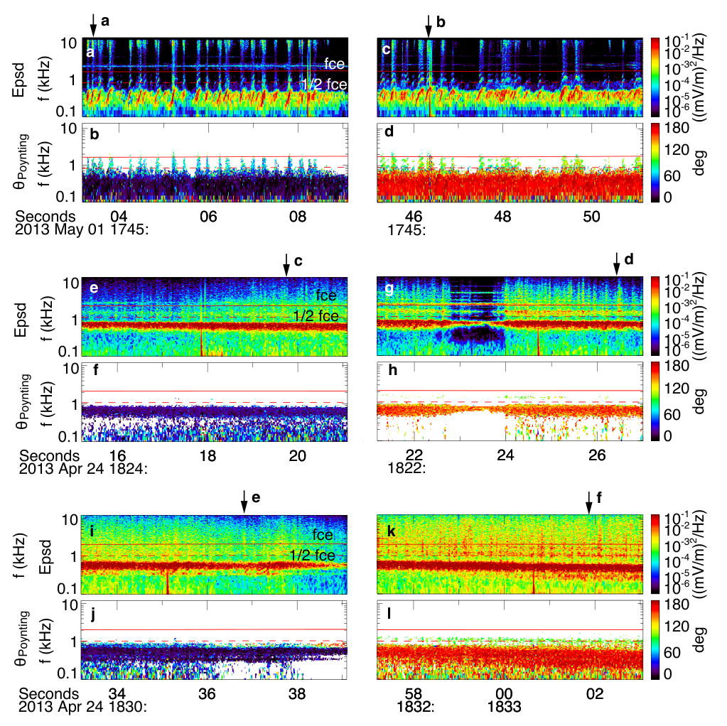
Fig. S1 presents the spectrograms of electric wave power and Poynting flux direction for whistler-related Langmuir waves [Fig. S1(a)-(d)], unipolar electric fields [Fig. S1(e)-(h)] and bipolar electric fields [Fig. S1(i)-(l)], corresponding to Van Allen Probes observation in Fig. 1. From the left panels to the right panels in Fig. S1, the direction of Poynting flux changes from parallel to anti-parallel with respect to the background magnetic field. Consequently, Langmuir waves occur at the opposite chorus wave phase while unipolar and bipolar electric fields change to the opposite polarity as shown in Fig. 1. The features of spectral density are also consistent with those shown in Fig. 2(a), Fig. 3(a) and Fig. 5(a).
II Simulation setup
We used a spectral Darwin particle-in-cell code in this study, which was developed as part of the University of California, Los Angeles Particle-In-Cell (UPIC) framework Decyk 2007. The Darwin approximation neglects the transverse displacement current and hence eliminates light waves in the system, but does not affect the physics of whistler and electrostatic waves Kaufman and Rostler 1971; Nielson and Lewis 1976; Busnardo-Neto et al. 1977. The simulation has one dimension () in configuration space and three dimensions () in velocity space. The boundary conditions for both particles and fields are periodic. The time step is . The cell length is , where is the initial electron Debye length. The background magnetic field is oriented at with respect to -direction in the - plane. The electron cyclotron frequency is equal to . This uniform background magnetic field is used since the excitation of the nonlinear wave structures is typically observed in the region around the magnetic equator Li et al. 2017; Malaspina et al. 2018. The ions are treated as an immobile neutralizing background since they do not take part in the dynamics. An isotropic Maxwellian distribution is initialized for electrons. To observe the nonlinear electron trapping by whistler waves, we need to reduce the background field fluctuations to a low level compared to the chorus wave field. For this purpose, each cell contains at least electrons. Such computational cost is currently not affordable in two and three dimensional simulations. The detailed parameters specific for each simulation are listed in Table 1.
To set up the whistler wave field, we need a particle distribution that supports the wave field. To achieve this goal, we use an external pump electric field during a prescribed time interval. Therefore each electron experiences an external acceleration from the pump electric field given by
| (S1) |
Here and are the particle velocity and the pump electric field, respectively. is the elementary charge, is the electron mass and is time. We add the pump electric field to the self-generated electric field as the total electric field, and add the background magnetic field to the self-generated magnetic field as the total magnetic field. The total electric and magnetic fields are used in the particle push. The wave number and frequency of the pump field is and . is connected to the mode number through , meaning the pump field has wave lengths in the system. Here is the number of cells in the system and is the cell length. The associated wave magnetic field is set up naturally by the particle response. The time profile of the pump electric field is
| (S2) |
The pump field starts with a linear up-ramp until , then keeps a constant amplitude until and finally ends with a linear down-ramp until . The simulation stops at . The relative amplitude of the pump field, i.e., and , is determined by the dispersion relation of whistler mode. The magnitude and duration of the pump field is chosen so that the normalized magnetic field of the whistler wave reaches when the pump field is turned off. Such a large amplitude wave is needed to overcome the incoherent field fluctuations in the simulation. The parameters relevant to the pump field are listed in Table 1.
Finally, it is worthy to note that the setup of the problem in the simulation is a temporal problem whereas it is a spatial problem in the space environment. In other words, the nonlinear trapping occurs across the simulation domain but for a limited time span in simulations, while in the space environment it occurs in a limited spatial range but for a longer time span when the whistler waves propagate from lower to higher latitudes. Nevertheless, the underlying physics of nonlinear trapping is the same in both scenarios.
| Simulation 1 | ||||||
|---|---|---|---|---|---|---|
| Simulation 2 | ||||||
| Simulation 3 | ||||||
| Simulation 1 | ||||||
| Simulation 2 | ||||||
| Simulation 3 |