Classification of Local Chemical Environments from X-ray Absorption Spectra using Supervised Machine Learning
Abstract
X-ray absorption spectroscopy is a premier, element-specific technique for materials characterization. Specifically, the x-ray absorption near edge structure (XANES) encodes important information about the local chemical environment of an absorbing atom, including coordination number, symmetry and oxidation state. Interpreting XANES spectra is a key step towards understanding the structural and electronic properties of materials, and as such, extracting structural and electronic descriptors from XANES spectra is akin to solving a challenging inverse problem. Existing methods rely on empirical fingerprints, which are often qualitative or semi-quantitative and not transferable. In this study, we present a machine learning-based approach, which is capable of classifying the local coordination environments of the absorbing atom from simulated K-edge XANES spectra. The machine learning classifiers can learn important spectral features in a broad energy range without human bias, and once trained, can make predictions on the fly. The robustness and fidelity of the machine learning method are demonstrated by an average % accuracy across the wide chemical space of oxides in eight transition metal families. We found that spectral features beyond the pre-edge region play an important role in the local structure classification problem, especially for the late transition metal elements.
Keywords:
x-ray absorption near-edge spectroscopy, machine learning, first-principles calculations, crystal structure, chemical bonding, crystal symmetryI Introduction
Knowledge of material structures at the atomic scale is essential to understanding physical phenomena and material properties that can lead to practical applications. Specifically, key information about the local chemical environment (LCE) surrounding an atom, including symmetry, coordination number, bond length and bond angle, forms the fundamental basis that determines the electronic properties of materials. In order to resolve the structure-property relationship, the characterization of atomic structures and their dynamic changes under different thermodynamic conditions has become a primary target of experimental studies. Such efforts have made tremendous impact on many research fields, including superconductivity Jorgensen et al. 1987, ultrafast dynamics Cavalleri et al. 2001, energy storage Kang and Ceder 2009, and photocatalysis Peng et al. 2015. Recent progress in materials discovery using smart automation Tabor et al. 2018; Gubernatis and Lookman 2018 and in situ and operando experiments Meirer and Weckhuysen 2018 further highlights emerging challenges and opportunities of materials characterization in real time.
Amongst many experimental techniques (e.g. imaging, diffraction, and spectroscopy), the x-ray absorption near edge structure (XANES) is a premier tool for probing LCEs, because it is element specific, sensitive to local structural and electronic properties, and applicable under harsh experimental conditions Ankudinov et al. 2002; Rehr et al. 2009; Frenkel et al. 2012, making it a robust structure refinement method Ankudinov et al. 1998; Ankudinov et al. 2002; Bazin and Rehr 2003; Ciatto et al. 2011; Ma et al. 2012; Kuzmin and Chaboy 2014. Given the atomic arrangement of a sample (), its XANES spectra () can be determined through quantum mechanical laws () via the mapping . Extracting the information of the LCE () as a subset of from spectral data can be formulated as an inverse problem: . The solution of this inverse problem is highly nontrivial, because the spectral information in experimental XANES is not only abstract, but also averaged over the whole sample. Consequently, much of the success in the past has been achieved by using fingerprints established from empirical observations.
In this study, we focus on transition metal K-edge XANES, which carries rich information about the electronic transitions from the core level of the absorbing atom to unoccupied states. Since the 1940’s, extensive research has been carried out to correlate spectral features of K-edge XANES spectra, especially in the pre-edge region, to LCEs Srivastava and Nigam 1973; Yamamoto 2008. For example, Hanson et al. Hanson and Beeman 1949 observed distinct chemical shifts in the absorption edge of Mn K-edge XANES in Mn, MnS, MnO2 and KMnO4. Wong et al. Wong et al. 1984 showed linear relationships between the oxidation state of V and both pre-edge and absorption edge positions in the K edge. Farges et al. Farges et al. 1996; Farges et al. 1997; Farges et al. 2001 and Jackson et al. Jackson et al. 2005 conducted comprehensive studies of the correlation between pre-edge features and the coordination number in Ti, Fe and Ni compounds; they found that the pre-edge peak intensity decreases with increasing coordination number. For fixed coordination number, early 3 transition metal elements (Ti, V, Cr and Mn) have stronger pre-edge peaks than late transition metal elements (Fe, Co, Ni and Cu) overall Yamamoto 2008. Furthermore, while both pre-edge peak locations and intensities in Ti Farges et al. 1996 and Ni species Farges et al. 2001 exhibit a significant dependence on the coordination number, the pre-edge peak positions in Fe compounds are independent of coordination number Jackson et al. 2005.
From a theoretical standpoint, the pre-edge peak intensity can be understood qualitatively from quantum mechanical selection rules. The dominant contribution in K-edge XANES comes from dipole transitions, as the quadrupole terms are generally orders of magnitude smaller. The density of states corresponding to the pre-edge regions of 3 transition metals are derived primarily from their empty 3 bands, and direct transitions are dipole-forbidden, which implies a vanishing peak intensity. However, pre-edge peak intensity is enhanced when atomic, unoccupied and states hybridize. According to group theory, atomic mixing is allowed under Td symmetry, but is forbidden under Oh symmetry Cotton and Ballhausen 1956; Cotton and Hanson 1956. As a result, 3 transition metals with tetrahedral geometries tend to exhibit stronger pre-edge peak intensities than those with octahedral geometries. To this end, empirical diagrams have been compiled to classify four-, five- and six-coordinated Ti, Ni and Fe based on pre-edge peak positions and intensities Farges et al. 1996; Farges et al. 1997; Farges et al. 2001; Jackson et al. 2005; we will refer to this method as the empirical fingerprint approach.
Despite the wide range of applications of the empirical fingerprint approach, including classifying LCEs in crystals, amorphous systems Farges et al. 1997; Mountjoy et al. 1999 and catalysts Bordiga et al. 2013, it has several limitations that may hinder its practical applications in the broader materials domain. First, coordination number is not the only factor that affects pre-edge peak features. Quantitative pre-edge features are determined by multiple factors, including coordination number, local distortion, oxidation state, and the nature of the ligands Jiang et al. 2007. For example, local distortions, e.g. displacements from the inversion center in octahedral geometries, under the crystal field can lower the local symmetry and enable atomic mixing, resulting in dramatic enhancement of pre-edge peak intensity Jiang et al. 2007. Such local distortion-induced pre-edge peak intensity enhancement has been reported in the V K-edges of six-coordinated MgV2O6 Yoshida et al. 1992 and NaV10O28 Tanaka et al. 1988, and in the Ti K-edge of six-coordinated Li4Ti5O12 Zhang et al. 2017. Therefore, isolating pure LCE effects and extracting robust correlations between the LCE and simple spectral descriptors, although valid for exemplary systems, may not be feasible for more structurally complex ones.
Secondly, the empirical fingerprint approach relies on human knowledge to engineer spectral descriptors, which may introduce bias. For example, existing spectral descriptors are primarily derived from the pre-edge region (e.g. peak positions and intensities). However, it is known that pre-edge features are much less visible in late transition metals than early transition metals Yamamoto 2008. Therefore, existing empirical fingerprint approach may not work effectively for late transition metals due to poor spectral contrast in the pre-edge region. One may need to systematically explore main- and post-edge spectral features in order to engineer and optimize new descriptors, which may not necessarily be simple ones, to tackle this problem.
Machine learning (ML) methods are a promising candidate to solve this inverse materials characterization problem. Instead of relying on empirical features derived from a small number of human observations, ML methods are data-driven approaches that make predictions based on large training sets, eliminating human bias from the feature selection process. There are myriad successful examples of the utilization of ML methods in condensed matter physics, materials science and chemistry, including methods to solve many-body problems Carleo and Troyer 2017, predict quantum phase transitions van Nieuwenburg et al. 2017, generate force field potentials Behler and Parrinello 2007, design new catalysts Kitchin 2018, and perform structure refinement Timoshenko et al. 2017; Timoshenko et al. 2018a. In the context of XANES, one expects ML algorithms to learn spectral descriptors in the full energy range of the spectrum and weight them appropriately for robust LCE predictions.
In this study, we tackled the LCE classification problem using supervised ML applied to a wide energy range of the XANES spectra ( eV above the onset) as input. In this way, the spectral feature space was systematically explored in order to establish the relationships between XANES spectra and LCE classes, specifically the local atomic geometries. As proof-of-principle, we applied ML algorithms to synthetic K-edge XANES spectra obtained from high throughput ab initio calculations. This study serves as a precursor to a potentially very powerful tool for real time structure refinement using experimental XANES, which will require in-depth understanding of the accuracy of the theory and further improvement of the ML algorithms.
II Methods
The workflow of the element-specific, spectrum-based LCE classification framework is summarized in Figure 1, which contains three core modules: data acquisition, LCE class labeling and training of machine learning models. We stress that the workflow we developed can be adapted to a wide range of elements characterized by different spectroscopic techniques, as long as the spectral information is element specific and sensitive to the LCE such that there exists distinguishable spectral contrast associated with different LCEs. Below, we describe each module in detail.
II.A Data Acquisition
For any given element, the first step is to extract atomic structures representing different LCEs from existing materials structure databases. The structural database must be large enough to build a reasonably-sized training set for machine learning models. To demonstrate the applicability of the LCE classification framework, we have considered eight 3 transition metal elements (Ti, V, Cr, Mn, Fe, Co, Ni, and Cu) and extracted all available oxide structures that have been structurally optimized using density functional theory (DFT) from the Materials Project Database Jain et al. 2013; Ong et al. 2013; Ong et al. 2015.
Once the structural database is established, the next step is to generate the corresponding spectral database. We focused on the K-edge XANES, as it is element specific and sensitive to the LCE (e.g., symmetry, charge state, and coordination number). In principle, one may populate the spectral database entirely with experimental spectra, but this strategy suffers from several drawbacks. First, experimental XANES spectra represent an average of signals (site-averaged signals) from each absorbing site (site-specific signals). In order to identify the correlations between spectra and local structures using ML, it is necessary to use site-specific spectra for training, as they possess much stronger spectral contrast than the site-averaged spectra. Second, when developing LCE classifiers using supervised ML methods, one needs to label XANES spectra with LCE descriptors, which means that only experimental spectra of known structures can be selected for the database. This requirement severely limits the pool of candidates for the database to mostly well-characterized crystal structures. As a result, qualified experimental spectra represent only a small fraction of the targeting LCEs in the local configuration space, which are heavily weighted in known crystals and under-represent the materials space of amorphous systems, surfaces, interfaces and nanoparticles. Consequently, a pure experimental spectral database suffers from data availability and data heterogeneity issues.
On the other hand, combined with available structural databases and well-established structure sampling methods, computational XANES have a clear advantage in exploring the LCE space and producing site-specific spectra. Furthermore, recent development in computational XANES modeling Rehr and Albers 2000; Taillefumier et al. 2002; Gougoussis et al. 2009; Prendergast and Galli 2006; Chen et al. 2010; Vinson et al. 2011; Vinson et al. 2014; Gulans et al. 2014; Vorwerk et al. 2017; Liang et al. 2017; Sun et al. 2018 has made it feasible to contrast experimental spectra quantitatively, enabling accurate local structure refinement of nanoparticles Timoshenko et al. 2017; Timoshenko et al. 2018b, interfaces Small et al. 2014, dopant sites Timoshenko et al. 2016; Singh et al. 2018 and structural phase transformation Zhang et al. 2017; Timoshenko et al. 2018a using computational techniques. An accurate and computationally efficient first-principles XANES method would be an ideal choice for sampling the vast LCE parameter space and mitigating data availability and heterogeneity issues. Indeed, computational XANES databases have recently emerged as a new tool for fast structure screening through data mining Mathew et al. 2018; Zheng et al. 2018; Yan et al..
In this study, we generated the computational XANES database with the FEFF9 code Rehr et al. 2010, which is a popular and computationally efficient method based on multiple scattering theory. We utilized the existing site-specific x-ray absorption spectroscopy FEFF library in the Materials Project Mathew et al. 2018; Zheng et al. 2018 and only calculated spectra not contained in this library. In the first data standardization step, site-specific spectra that failed sanity checks were automatically discarded, such as when the FEFF calculations did not converge with the default input or when the output FEFF spectra are not physical (e.g., with negative absorption coefficients). In the second step, we removed “duplicates”, which otherwise would have introduced bias if nearly identical structures were selected for both training and testing. We used a site-symmetry finder from the pymatgen library Ong et al. 2013 to determine which sites in a crystal structure are symmetrically equivalent. For every pair of spectra, one was removed from the dataset if the average mean absolute difference between them was less than , a number chosen based on visual inspection of a large number of similar spectra. The process of removing duplicates also has the benefit of reducing the total number of necessary FEFF calculations to populate the XANES database. Finally, calculated XANES spectra were spline-interpolated onto an absorbing site-specific energy grid, so that the input feature vector was standardized for each spectrum. For each type of absorbing site, the energy grid was chosen such that it contains the maximum amount of available information with an energy resolution of approximately 0.5 eV.
All standardized data before augmentation are henceforth referred to as the base dataset. Training data were augmented by shifting the spectra by and eV. The size of the augmented training set thus becomes five times the size of the base dataset. We found that data augmentation improves the accuracy and robustness of the machine learning model.
II.B Local Chemical Environment Class Labeling
Feature engineering of LCEs is an active research topic with increasing applications in a variety of areas including, for example, neural network potential development Behler and Parrinello 2007; Rupp et al. 2012; Smith et al. 2017; Chmiela et al. 2017. Among many possible choices, labels based on the coordination environment (e.g. tetrahedral, square pyramidal, and octahedral geometries), although simple, provide key information on chemical bonding and have been widely used in the x-ray spectroscopy community. In this study, we utilized the continuous symmetry measure (CSM), developed by Avnir and Pinsky Pinsky and Avnir 1998 and hosted in the ChemEnv package Waroquiers et al. 2017, to measure the similarity between an input local geometry and a particular polyhedron. The smaller the CSM for a polyhedron, the more the input geometry resembles it. We applied a cutoff such that atoms further away than times the nearest neighbor distance from the absorbing site were not considered. This cutoff was chosen as a balance between prediction accuracy and computational cost. The CSM was applied to each absorbing site, and the polyhedron with the lowest CSM value was chosen as the site LCE label.
We restricted the LCE labels to only tetrahedral (T4), square pyramidal (S5) and octahedral (O6) geometries, because across the eight transition metal families these are the most abundant LCEs, often by an order of magnitude more than the rest. The class breakdown of the dataset is presented in Table 1. The total number of site-specific spectra is on average a few thousand per atom type, with V (3366) and Mn (3493) the most abundant and Cu (839) the least abundant. It should be noted that one can expand the dataset by adding new structures from other material databases, generating artificial structures or introducing additional class labels. Furthermore, amongst all three chosen classes, O6 dominates, making up about % of the entire structure database. The impact of the inhomogeneity of the data distribution on the predictive power of the ML model is discussed in Section III.
| Absorber | T4 | S5 | O6 | Total |
|---|---|---|---|---|
| Ti | 271 | 359 | 1562 | 2192 |
| V | 948 | 412 | 2006 | 3366 |
| Cr | 396 | 121 | 902 | 1419 |
| Mn | 502 | 657 | 2334 | 3493 |
| Fe | 797 | 319 | 1874 | 2990 |
| Co | 583 | 227 | 1428 | 2238 |
| Ni | 246 | 163 | 1238 | 1647 |
| Cu | 290 | 183 | 366 | 839 |
| Total | 4033 | 2441 | 11710 | 18184 |
II.C Training Machine Learning Models
The core machine learning algorithm (see Figure 1) consists of an optional 1-D convolutional layer followed by three fully connected, feed-forward hidden layers with 90, 60 and 20 neurons, ending with a softmax output layer of 3 neurons. The input layer of the neural network is the XANES spectrum scaled to zero mean and unit variance on a standardized grid of 100 entries, and the output determines the target vector, which contains the probabilities of the three LCE classes (T4, S5 and O6) computed from the softmax function. All neurons use the rectified linear unit (ReLU) activation function and a % dropout to guard against over-fitting. ML models with and without the 1-D convolutional layer are referred to as the convolutional neural network (CNN) and multi-layer perceptron (MLP), respectively. The optional convolutional layer contains 8 filters and a kernel (sliding window) size of 10, stride of 1 and max-pooling size of 2, and takes as input spectral data processed in an identical manner to that of the MLP. CNN’s inherently assume correlations between nearby data points, and being a down-sampling and pooling technique, sacrifice resolution in favor of invariance to the precise location of input data. The algorithm determines trained parameters by minimizing a categorical cross-entropy loss function using the Adam optimizer Kingma and Ba 2014. Mini-batch sizes of 32 were used during 50 full passes (epochs) of the training data. All training and evaluations were performed using Keras Chollet et al. 2015 with a TensorFlow Abadi et al. 2015 backend.
For each absorbing site, we used statistical boostrapping. % of the database was used for training ML models and the remainder for testing. These subsets were selected randomly in a stratified manner: the proportion of each class in both the training and testing sets was always the same. In order to generate a statistical estimate on the accuracy of the classifier, we sampled the testing data with replacement over folds and report the averaged results in Figure 3. To make full use of all available information, data included once in a testing set, were not used in any future testing sets. We found that testing results are mostly invariant to the chosen neural network architecture assuming enough training parameters were included. Therefore, the fixed 3-layer MLP with an optional convolutional layer (and associated hyperparameters) was used throughout all experiments.
III Results and Discussion
In the following, we present our LCE classification study through visual inspection, principal component analysis (PCA) Pearson 1901 and analysis of the machine learning classifiers (MLCs). We demonstrate that MLCs can accurately predict LCE classes from synthetic XANES data generated by FEFF. We further discuss the relevance of this study based on synthetic data to the real challenge of the LCE classification of experimentally measured XANES spectra.
III.A Visual Inspection of the Spectral Database

The FEFF K-edge XANES database of eight transition metal elements (from Ti to Cu) is shown in Figure 2, color coded by LCE class (T4: blue; S5: green; O6: red). There are noticeable trends in the raw spectra that can be detected by visual inspection, prior to a more in-depth analysis. Overall, early transition metals (e.g. Ti, V, Cr, and Mn) show more intense pre-edge peaks than late transition metals (e.g. Ni and Cu), consistent with the trend from experiment Yamamoto 2008. Notably, T4 in Ti, V and Cr oxides exhibit sharp pre-edge peaks at about , , and eV, respectively. The pre-edge peak intensity decreases as the coordination number increases, consistent with the observations of Farges et al. Farges et al. 1996; Farges et al. 1997; Farges et al. 2001 and Jackson et al. Jackson et al. 2005. Such qualitative agreement between theory and experiment suggests that spectral analysis of the FEFF database is physically insightful, especially for the LCE classification problem.
In addition to pre-edge features, across the eight elements T4 exhibits the highest post-edge intensity, followed by S5 and finally O6. However, the role of post-edge features in LCE classification has not yet been explored in the literature, which could be an important supplement to existing pre-edge based methods. We expect that algorithms including a wide energy range in the XANES spectra can in principle improve the spectral sensitivity to the LCE as compared to those relying solely on pre-edge features.
III.B Principal Component Analysis of the Spectral Database
We further analyzed the spectral database with PCA. Following the standard notation, is defined as the full set of spectral data for the th absorbing species with being the th spectrum in the dataset (a single feature vector input) after taking zero sample mean and unit variance. Denote and as the first two principal axes in the feature space. We computed coordinates of spectrum in the PCA plot, , as
| (1) |
where for clarity the denominator scales within .
To evaluate the significance of the pre-edge features, we truncated the principal axes by applying a cutoff to the spectra, such that correspond to the vertical dashed lines in Figure 2. Then PCA was performed for only the pre-edge region along the truncated principal axes,
| (2) |
by excluding features beyond . The axes in the plots generated by Eqs. 1 and 2 are scaled in the same way, so that their clustering patterns can be compared directly. Similar patterns are expected from the full and pre-edge PCA plots, if the pre-edge features dominate the spectral contrast. On the other hand, if the pre-edge features are less significant, there will be weak correlations between two sets of PCA patterns.
Full PCA plots are shown in the lower right insets of Figure 2. Overall, a large degree of clustering is realized, consistent with the observation of distinguishable spectral features from visual inspection. In Ti, V, Cr, Mn, Fe, and Co, most of the T4 points are located in the lower right corner and O6 points in the upper left corner. The T4 and O6 points of the Ti, V, and Cr can be easily separated in PCA plots due to their sharp (T4) and negligible (O6) pre-edge features. In the PCA plots of Mn, Fe and Co, there is also a secondary cluster of T4 points located in the upper right corner. The data distributions in Ni and Cu are similar to the others, but with a slightly smaller packing density. In most cases, S5 clusters are intertwined with the other two classes, flanked by T4 on one side and O6 on the other.
The lower center insets in Figure 2 show the PCA of the pre-edge region. All classes appear less clustered than the PCA patterns of the full feature space. While in this case information contained in the feature space has clearly been reduced, this effect is less prominent in the early transition metal elements, which still exhibit a large degree of clustering due to the significant spectral contrast in the pre-edge region. On the contrary, elements such as Co, Ni and Cu exhibit such severe information loss that PCA data points collapse into a linear pattern, which is detrimental to the MLC performance, especially in systems that already exhibit weak spectral contrast.
In summary, visual inspection and PCA suggest that a MLC is likely able to accurately learn the trends in XANES spectra and correlate them to their respective classes. However, it is unclear whether MLCs can perform equally well for every class in all of the transition metal species we studied.
III.C Performance of the Machine Learning Classifiers
The accuracy of the MLCs for each LCE class is reported using the score, which is the harmonic mean of the precision and recall
| (3) |
where and represent the true positives, false positives and false negatives in a two-class (2 by 2) confusion matrix.
In order to make a fair assessment of the MLC performance, we need to address the data imbalance issue in our training set. As seen in Table 1, the number of LCEs that conform to the O6 geometry vastly outnumbers the others, indicating that the accuracy of each class alone might not be the most reliable metric, as it may be biased due to class imbalances in the training data. We address this problem in two ways: by using the score instead of the accuracy on a class-by-class basis, and reporting the macro score as a representative metric.
In general, the score is a much stricter metric than the accuracy and is a better indicator of performance. It accounts for both the precision (of all predicted positives, cases that are actually positive) and recall (out of all the actual positives, cases that are correctly identified) and dramatically penalizes poor scores in either category (contrary to the mean of the precision and recall). To demonstrate why this is important, consider the score of the relatively underrepresented S5 class. Suppose that there are 10 S5 and 100 T4 and O6 in the data set, and that the classifier has a 10% false negative and false positive rate. Accuracy would naturally be 90%, but this is a terrible representation of the classifier, since 10 non-S5 data points were predicted as S5, unnaturally inflating the number of predicted positives. On the contrary, the score of 62% accounts for this by incorporating the low precision (47%) into the metric.
In addition to a breakdown by class, the macro score () is reported, which is the average of the class-wise scores computed using a one-versus-all approach. The score treats each class on equal footing and further penalizes classifying data in an underrepresented class incorrectly relative to a class with many data points.
| Full Feature Space | Pre-edge Only | |||
|---|---|---|---|---|
| Element | MLP | CNN | pre-MLP | pre-CNN |
| Ti | 0.83(2) | 0.84(2) | 0.73(4) | 0.78(3) |
| V | 0.86(1) | 0.86(2) | 0.77(2) | 0.79(3) |
| Cr | 0.87(2) | 0.87(3) | 0.72(4) | 0.75(4) |
| Mn | 0.83(2) | 0.85(2) | 0.62(4) | 0.68(3) |
| Fe | 0.85(2) | 0.86(3) | 0.57(2) | 0.63(3) |
| Co | 0.85(3) | 0.87(2) | 0.59(3) | 0.64(3) |
| Ni | 0.87(1) | 0.88(3) | 0.61(5) | 0.66(4) |
| Cu | 0.86(2) | 0.86(2) | 0.50(4) | 0.64(7) |
| Average | 0.85(1) | 0.86(1) | 0.64(1) | 0.70(1) |
As clearly shown from the scores in Table 2, MLCs can classify the LCEs of all eight transition metal families very accurately. Uncertainties reported in the last digit of Table 2 and error bars in Figure 3 correspond to the standard deviation calculated from ten different trained models. CNNs and MLPs perform equally well, with very close scores of 0.86 and 0.85, respectively. The class-wise scores are plotted in Figure 3. Notably, MLCs can reach over % accuracy on the T4 (CNN: 0.92; MLP: 0.92) and O6 classes (CNN: 0.96; MLP: 0.95), which can be understood from the observation of raw spectra. The strong pre-edge peak intensity is a signature of the T4 configuration in, e.g., Ti, V and Cr. Conversely, the lack of a significant pre-edge peak is a clear indicator of an O6 configuration. In these cases, it is likely that the pre-edge features are sufficient to distinguish O6 from T4. On the contrary, the spectral contrast between T4 and O6 is very low in the pre-edge region in late transition metal elements, especially in Ni and Cu. It is remarkable that MLCs can achieve the same accuracy for T4 and O6 in late transition metal elements. Such a universally good performance underscores the ability of the MLCs to extract spectral descriptors without human bias in the full energy range, including the pre-, main- and post-edge regions. Moreover, the relatively small overall error margin is a testament to the reliability and robustness of the classifier across many trained models.
Relatively speaking, the S5 classification is less successful than T4 and O6, with an overall accuracy of (CNN: 0.71; MLP: 0.68), as shown in Figure 3. The weaker performance of MLCs on the S5 class can be explained by Figure 2, where data associated with the S5 class lay between those in T4 and O6 in both the spectral and principal component space, making them more difficult to identify.

III.D Importance of Features Beyond the Pre-edge
The ability of MLCs to accurately classify late transition metal oxides that lack prominent pre-edge features suggests that features beyond the pre-edge region play an important role in the neural network model. This hypothesis is supported by the PCA results shown in the insets of Figure 2. In the late transition metals, while the full spectra can be effectively clustered in two-component PCA, the same analysis of pre-edge spectra displays a completely different linear pattern resulting from substantial information loss.
To gain further insight, we train MLCs with identical architectures using only the pre-edge region defined by energies below the dashed lines in Figure 2, which we refer to as the pre-MLCs (pre-CNNs and pre-MLPs). In principle, if scores of the pre-MLCs are close to those trained on the full spectra, then the pre-edge features are sufficient to classify the LCE for that absorbing element. Conversely, a significant drop in the scores of the pre-MLCs would be a clear indication that features beyond the pre-edge region play a significant role in the MLCs.
As shown in Table 2, the average score in pre-MLCs drops significantly by about % (from to in CNN and from to in MLP), as compared to MLCs trained on the full spectral space. The class-wise scores of pre-MLCs which are consistently lower than that of regular MLCs are shown in Figure 3 as the gray bars. We quantify this accuracy degradation by
and summarize the results averaged over early (Ti, V, Cr, and Mn) and late transition metal elements (Fe, Co, Ni and Cu) in Table 3. First, in late transition metals is more than doubled compared to early transition metals. Second, among the three classes, of O6 is the smallest (). It increases significantly for T4 in late transition metals to in the pre-CNN ( in the pre-MLP) and finally reaches the largest values for S5, at () in early transition metals and () in late transition metals. The results in Figure 3 and Tables 2-3 highlight the critical importance of features beyond the pre-edge region in accurately classifying LCEs, especially for late transition metals. The effects are the largest in the S5 class, which is rather characterless in the pre-edge region, showing neither very strong (like T4) nor very weak (like O6) pre-edge intensities.
| pre-MLP | pre-CNN | |||||
|---|---|---|---|---|---|---|
| T4 | S5 | O6 | T4 | S5 | O6 | |
| Early | 0.09(3) | 0.30(5) | 0.03(1) | 0.07(3) | 0.22(5) | 0.03(1) |
| Late | 0.21(4) | 0.57(5) | 0.10(1) | 0.16(3) | 0.44(7) | 0.08(1) |
We note that unlike the case of regular MLCs, the pre-edge CNN averaged over all absorbing species () outperforms the corresponding pre-edge MLP () substantially. In the most extreme situation of S5, the pre-CNN () is % more accurate than the pre-MLP () in early transition metals, and it is more than doubled in late transition metals with for the pre-CNN (pre-MLP). The substantially better performance of the pre-CNN is likely caused by the use of the convolutional filter, which makes the CNN able to learn subtle pre-edge features from augmented data more effectively than the MLP.
III.E Discussion
The MLCs described so far were trained on computational FEFF XANES spectra. Developing MLCs that can classify the LCE of a broad range of material families using experimental XANES spectra is a more challenging task that is beyond the scope of the current work. Nonetheless, in this section we discuss several key issues that need to be addressed in order to achieve this goal, including validation of the theory, edge alignment of the simulated spectra, and the variations in the spectral intensity.
In order to appy MLCs trained on synthetic data to experimental spectra, it is very important to validate the theory such that the computational spectra can faithfully reproduce experimental spectral features. To this end, we compare FEFF spectra with experimental spectra on a small number of oxides: K6Ti2O7, rutile (TiO2), MnCr2O4, MnCO3, CoAlO4 and Co(AsO4)2 in Figure 4. This list is not meant to be exhaustive. Within this small sample, while the overall shape and major peaks are well reproduced by FEFF, there are noticeable differences in the spectral details, including the peak positions and relative intensities of different peaks. Furthermore, the degree of agreement is system-dependent. As shown in Figure 4, the optimal Pearson correlation coefficients (PCCs) between FEFF and experiment range from to .
Despite the relatively high PCC scores, MLCs trained on spectra at the FEFF level of theory as such cannot reliably classify experimental spectra. It is necessary to generate the computational XANES database with more accurate methods and conduct a systematic benchmark of theory against experiment. However, the computational expense of these calculations grows quickly with the complexity of the methods, which could in practice limit the level of theory used to generate the training set. A good compromise would involve developing robust ML algorithms for a physically sound but numerically imperfect training set. It may also be possible to augment the computational spectral database with a subset of experimental data and apply ML techniques that can handle a hybrid database, such as transfer learning.
Another open question in computational XANES is the edge alignment of computational spectra with experimental spectra, because current first-principles electronic structure methods have difficulty predicting accurate absolute onset energies. This issue stems from the use of pseudopotentials and/or approximations to the electron self-energy and core-hole final state effects. Therefore, XANES calculations are often analyzed with the relative energy scale or after they are manually aligned with reference experimental spectra. However, the energy shift in the spectral alignment with respect to reference experimental spectra could be system-dependent, which warrants further study.
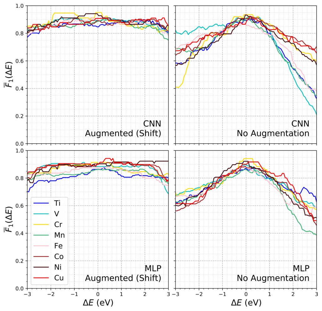
In order to investigate the impact of the edge alignment on the performance of MLCs, we shift the test set by up to eV to study the transferability of MLCs against the shifted data. We note that a shift of eV in energy is quite significant, as the energy range of the pre-edge region is about to eV. As shown in Figure 5, the MLCs are very robust against the energy shift, as the curves are almost flat. The CNN slightly outperforms MLP with (CNN) in most of the range of for all eight elements. The robustness of the MLCs results from the data augmentation we applied in the training set with energy shifts of and eV as described in the Section II. If we apply the same test on MLCs developed from the base training set without data augmentation, the accuracy deteriorates quickly after eV, as shown in Figure 5.
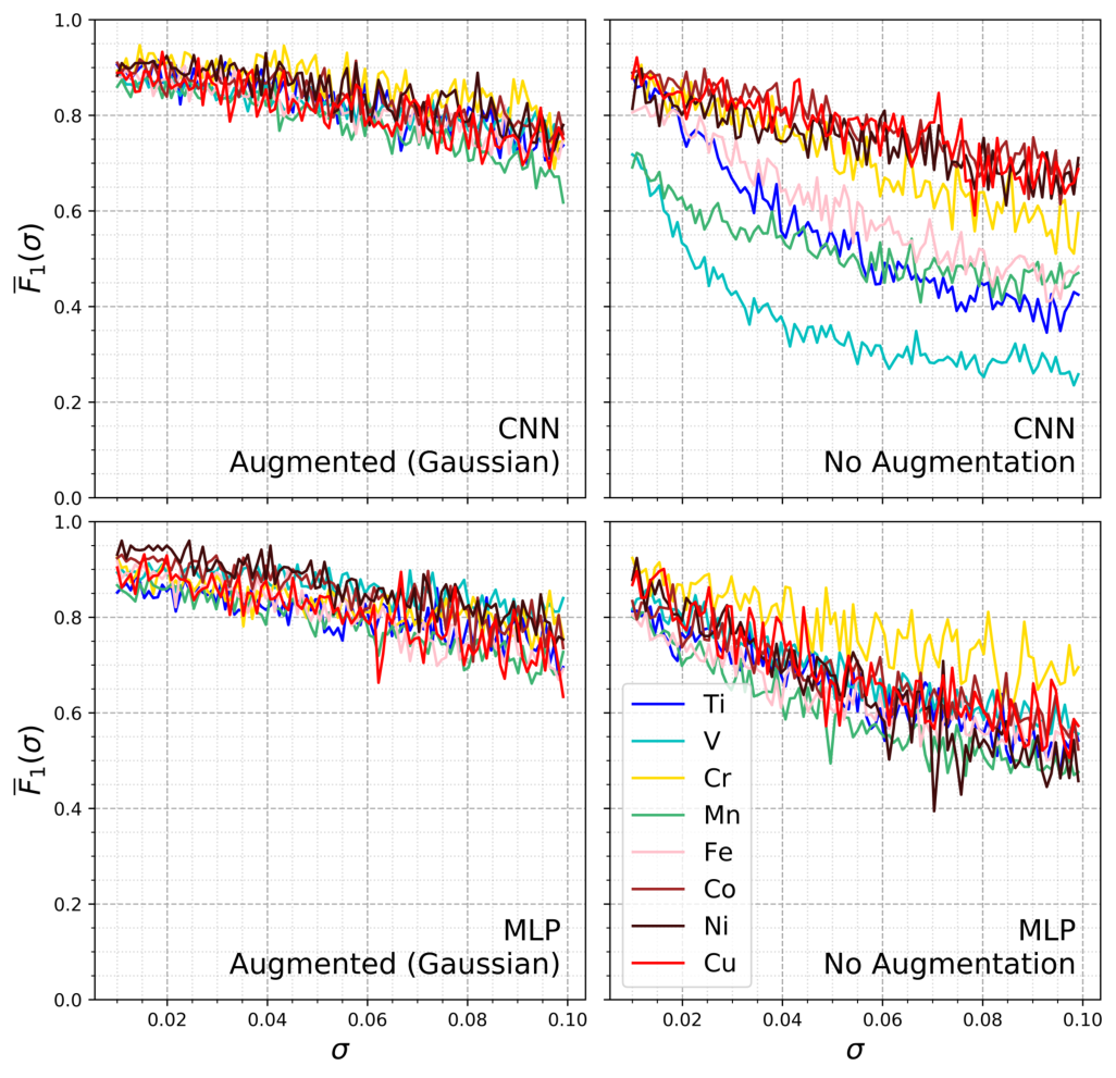
Additionally, we have seen that the spectral intensity of theoretical XANES spectra may not match perfectly with experiments. On top that, the intensity of experimental XANES spectra is subject to several uncertainties from sample preparation and various instrumental factors, such as type and mosaic spread of the monochromator crystals, source sizes, slit heights and beam instabilities Farges et al. 1997 and the resolution of the apparatus Yoshitake et al. 2003. Therefore, experimental spectra of the same materials that are measured using different samples or collected at different beamline settings may have slightly different intensity profiles. To investigate the impact of the uncertainties in the spectral intensity on the MLCs, we introduced Gaussian random noise with standard deviation to the spectral intensity centered around for every on the energy grid. To isolate the effects of the Gaussian random noise, we test the MLCs trained without augmentation accounting for the energy shift. As shown in Figure 6, the overall score decays quickly with the increasing in both the CNN and MLP, with V trained using the CNN suffering the most. After we augmented the training set with spectra containing the Gaussian random noise with , the score decays much more slowly with increasing .
From the analysis above, one can clearly see that MLCs perform dramatically better when the training set is augmented, which is a sensible result. It is interesting to note that the CNN underperforms relative to the MLP without data augmentation, specifically for early transition metals that exhibit strong pre-edge peaks. For example, the score of the unaugmented CNN for Ti and V drops to and , respectively, at . This trend is not entirely counterintuitive for two reasons. First, the CNN as described in Subsection II.C is not completely shift-invariant, and without proper data augmentation it may not learn how to account for small perturbations. Second, as shown in Table 3, the CNN relies more on the pre-edge region than the MLP. Since shifting the location of the pre-edge peak strongly affects the pre-edge spectral features, a sizable drop in performance is to be expected. A similar argument may be made for the effects of Gaussian random noise, which can artificially distort both the shape and location of peaks.
IV Conclusion
We propose a new computational framework to perform element-specific classification of local chemical environments from XANES spectra. In addition to the construction of structure and spectral databases and structural labels, a central element of this framework is unraveling the correlation between spectral features and local chemical environments systematically using machine learning classifiers. As proof-of-principle, we applied our method to the computational XANES database of eight 3 transition metal elements generated by the FEFF code and achieved a high average macro score of . Our method can reliably capture not only the prominent pre-edge features, but also the less characteristic spectral features beyond the pre-edge region. We showed that features beyond the pre-edge region turn out to be very important to the accuracy of the classification, especially for late transition metal elements. The ability to extract key structural information in the full spectral range makes our machine learning-based method more robust and transferable than empirical fingerprint methods based solely on the pre-edge region. As an important starting point, our work will motivate future research on the problem of classification of local chemical environments on experimental measured spectra.
Acknowledgements.
This research used resources of the Center for Functional Nanomaterials, which is a U.S. DOE Office of Science Facility, and the Scientific Data and Computing Center, a component of the BNL Computational Science Initiative, at Brookhaven National Laboratory under Contract No. DE-SC0012704. This research is also, in part, supported by Brookhaven National Laboratory LDRD (Lab Directed Research and Development) 16-039. M.R.C. acknowledges support from the U.S. Department of Energy through the Computational Sciences Graduate Fellowship (DOE CSGF) under grant number: DE-FG02-97ER25308. The authors acknowledge fruitful discussions with Mark Hybertsen, Anatoly Frenkel, Bruce Ravel, Klaus Attenkofer, Eli Stavitski, Xiaochuan Ge, Sencer Selcuk and Marco Baity-Jesi.References
- Jorgensen et al. (1987) J. D. Jorgensen, M. A. Beno, D. G. Hinks, L. Soderholm, K. J. Volin, R. L. Hitterman, J. D. Grace, I. K. Schuller, C. U. Segre, K. Zhang, and M. S. Kleefisch, Phys. Rev. B 36, 3608 (1987).
- Cavalleri et al. (2001) A. Cavalleri, C. Tóth, C. W. Siders, J. A. Squier, F. Ráksi, P. Forget, and J. C. Kieffer, Phys. Rev. Lett. 87, 237401 (2001).
- Kang and Ceder (2009) B. Kang and G. Ceder, Nature 458, 190 (2009).
- Peng et al. (2015) H. Peng, P. F. Ndione, D. S. Ginley, A. Zakutayev, and S. Lany, Phys. Rev. X 5, 021016 (2015).
- Tabor et al. (2018) D. P. Tabor, L. M. Roch, S. K. Saikin, C. Kreisbeck, D. Sheberla, J. H. Montoya, S. Dwaraknath, M. Aykol, C. Ortiz, H. Tribukait, et al., Nat. Rev. Mater. 3, 5 (2018).
- Gubernatis and Lookman (2018) J. E. Gubernatis and T. Lookman, Phys. Rev. Mater. 2, 120301 (2018).
- Meirer and Weckhuysen (2018) F. Meirer and B. M. Weckhuysen, Nat. Rev. Mater. 3, 324 (2018).
- Ankudinov et al. (2002) A. Ankudinov, J. Rehr, J. J. Low, and S. R. Bare, J. Chem. Phys. 116, 1911 (2002).
- Rehr et al. (2009) J. J. Rehr, J. J. Kas, M. P. Prange, A. P. Sorini, Y. Takimoto, and F. Vila, Comptes rendus Phys. 10, 548 (2009).
- Frenkel et al. (2012) A. I. Frenkel, J. A. Rodriguez, and J. G. Chen, ACS Catal. 2, 2269 (2012).
- Ankudinov et al. (1998) A. L. Ankudinov, B. Ravel, J. J. Rehr, and S. D. Conradson, Phys. Rev. B 58, 7565 (1998).
- Bazin and Rehr (2003) D. Bazin and J. J. Rehr, J. Phys. Chem. B 107, 12398 (2003).
- Ciatto et al. (2011) G. Ciatto, A. Di Trolio, E. Fonda, P. Alippi, A. M. Testa, and A. A. Bonapasta, Phys. Rev. Lett. 107, 127206 (2011).
- Ma et al. (2012) Q. Ma, J. Prater, C. Sudakar, R. Rosenberg, and J. Narayan, J. Phys.: Condens. Matter 24, 306002 (2012).
- Kuzmin and Chaboy (2014) A. Kuzmin and J. Chaboy, IUCrJ 1, 571 (2014).
- Srivastava and Nigam (1973) U. Srivastava and H. Nigam, Coord. Chem. Rev. 9, 275 (1973).
- Yamamoto (2008) T. Yamamoto, X-Ray Spectrom. 37, 572 (2008).
- Hanson and Beeman (1949) H. Hanson and W. W. Beeman, Phys. Rev. 76, 118 (1949).
- Wong et al. (1984) J. Wong, F. W. Lytle, R. P. Messmer, and D. H. Maylotte, Phys. Rev. B 30, 5596 (1984).
- Farges et al. (1996) F. Farges, G. E. Brown Jr, and J. J. Rehr, Geochim. Cosmochim. Acta 60, 3023 (1996).
- Farges et al. (1997) F. Farges, G. E. Brown, and J. J. Rehr, Phys. Rev. B 56, 1809 (1997).
- Farges et al. (2001) F. Farges, G. E. Brown Jr, P.-E. Petit, and M. Munoz, Geochim. Cosmochim. Acta 65, 1665 (2001).
- Jackson et al. (2005) W. E. Jackson, F. Farges, M. Yeager, P. A. Mabrouk, S. Rossano, G. A. Waychunas, E. I. Solomon, and G. E. Brown, Geochim. Cosmochim. Acta 69, 4315 (2005).
- Cotton and Ballhausen (1956) F. A. Cotton and C. J. Ballhausen, J. Chem. Phys. 25, 617 (1956).
- Cotton and Hanson (1956) F. A. Cotton and H. P. Hanson, J. Chem. Phys. 25, 619 (1956).
- Mountjoy et al. (1999) G. Mountjoy, D. M. Pickup, G. Wallidge, R. Anderson, J. M. Cole, R. J. Newport, and M. E. Smith, Chem. Mater. 11, 1253 (1999).
- Bordiga et al. (2013) S. Bordiga, E. Groppo, G. Agostini, J. A. van Bokhoven, and C. Lamberti, Chem. Rev. 113, 1736 (2013).
- Jiang et al. (2007) N. Jiang, D. Su, and J. C. H. Spence, Phys. Rev. B 76, 214117 (2007).
- Yoshida et al. (1992) S. Yoshida, T. Tanaka, T. Hanada, T. Hiraiwa, H. Kanai, and T. Funabiki, Catal. Lett. 12, 277 (1992).
- Tanaka et al. (1988) T. Tanaka, H. Yamashita, R. Tsuchitani, T. Funabiki, and S. Yoshida, J. Chem. Soc., Faraday Trans. 1 84, 2987 (1988).
- Zhang et al. (2017) W. Zhang, M. Topsakal, C. Cama, C. J. Pelliccione, H. Zhao, S. Ehrlich, L. Wu, Y. Zhu, A. I. Frenkel, K. J. Takeuchi, et al., J. Am. Chem. Soc. 139, 16591 (2017).
- Carleo and Troyer (2017) G. Carleo and M. Troyer, Science 355, 602 (2017).
- van Nieuwenburg et al. (2017) E. P. L. van Nieuwenburg, Y.-H. Liu, and S. D. Huber, Nat. Phys. 13, 435 (2017).
- Behler and Parrinello (2007) J. Behler and M. Parrinello, Phys. Rev. Lett. 98, 146401 (2007).
- Kitchin (2018) J. R. Kitchin, Nat. Catal. 1, 230 (2018).
- Timoshenko et al. (2017) J. Timoshenko, D. Lu, Y. Lin, and A. I. Frenkel, J. Phys. Chem. Lett. 8, 5091 (2017).
- Timoshenko et al. (2018a) J. Timoshenko, A. Anspoks, A. Cintins, A. Kuzmin, J. Purans, and A. I. Frenkel, Phys. Rev. Lett. 120, 225502 (2018a).
- Jain et al. (2013) A. Jain, S. P. Ong, G. Hautier, W. Chen, W. D. Richards, S. Dacek, S. Cholia, D. Gunter, D. Skinner, G. Ceder, and K. A. Persson, APL Mater. 1, 011002 (2013).
- Ong et al. (2013) S. P. Ong, W. D. Richards, A. Jain, G. Hautier, M. Kocher, S. Cholia, D. Gunter, V. L. Chevrier, K. A. Persson, and G. Ceder, Comput. Mater. Sci. 68, 314 (2013).
- Ong et al. (2015) S. P. Ong, S. Cholia, A. Jain, M. Brafman, D. Gunter, G. Ceder, and K. A. Persson, Comput. Mater. Sci. 97, 209 (2015).
- Rehr and Albers (2000) J. J. Rehr and R. C. Albers, Rev. Mod. Phys. 72 (2000).
- Taillefumier et al. (2002) M. Taillefumier, D. Cabaret, A.-M. Flank, and F. Mauri, Phys. Rev. B 66, 195107 (2002).
- Gougoussis et al. (2009) C. Gougoussis, M. Calandra, A. Seitsonen, C. Brouder, A. Shukla, and F. Mauri, Phys. Rev. B 79, 045118 (2009).
- Prendergast and Galli (2006) D. Prendergast and G. Galli, Phys. Rev. Lett. 96, 215502 (2006).
- Chen et al. (2010) W. Chen, X. Wu, and R. Car, Phys. Rev. Lett. 105, 017802 (2010).
- Vinson et al. (2011) J. Vinson, J. J. Rehr, J. J. Kas, and E. L. Shirley, Phys. Rev. B 83, 115106 (2011).
- Vinson et al. (2014) J. Vinson, T. Jach, W. T. Elam, and J. D. Denlinger, Phys. Rev. B 90, 205207 (2014).
- Gulans et al. (2014) A. Gulans, S. Kontur, C. Meisenbichler, D. Nabok, P. Pavone, S. Rigamonti, S. Sagmeister, U. Werner, and C. Draxl, J. Phys.: Condens. Matter 26, 363202 (2014).
- Vorwerk et al. (2017) C. Vorwerk, C. Cocchi, and C. Draxl, Phys. Rev. B 95, 155121 (2017).
- Liang et al. (2017) Y. Liang, J. Vinson, S. Pemmaraju, W. S. Drisdell, E. L. Shirley, and D. Prendergast, Phys. Rev. Lett. 118, 096402 (2017).
- Sun et al. (2018) Z. Sun, L. Zheng, M. Chen, M. L. Klein, F. Paesani, and X. Wu, Phys. Rev. Lett. 121, 137401 (2018).
- Timoshenko et al. (2018b) J. Timoshenko, C. J. Wrasman, M. Luneau, T. Shirman, M. Cargnello, S. R. Bare, J. Aizenberg, C. M. Friend, and A. I. Frenkel, Nano Lett. in press (2018b).
- Small et al. (2014) M. W. Small, J. J. Kas, K. O. Kvashnina, J. J. Rehr, R. G. Nuzzo, M. Tromp, and A. I. Frenkel, ChemPhysChem 15, 1569 (2014).
- Timoshenko et al. (2016) J. Timoshenko, A. Shivhare, R. W. J. Scott, D. Lu, and A. I. Frenkel, Phys. Chem. Chem. Phys. 18, 19621 (2016).
- Singh et al. (2018) H. Singh, M. Topsakal, K. Attenkofer, T. Wolf, M. Leskes, Y. Duan, F. Wang, J. Vinson, D. Lu, and A. I. Frenkel, Phys. Rev. Mater. 2, 125403 (2018).
- Mathew et al. (2018) K. Mathew, C. Zheng, D. Winston, C. Chen, A. Dozier, J. J. Rehr, S. P. Ong, and K. A. Persson, Sci. Data 5, 180151 (2018).
- Zheng et al. (2018) C. Zheng, K. Mathew, C. Chen, Y. Chen, H. Tang, A. Dozier, J. J. Kas, F. D. Vila, J. J. Rehr, L. F. Piper, et al., npj Comput. Mater. 4, 12 (2018).
- (58) D. Yan, M. Topsakal, S. Selcuk, J. Lyons, W. Zhang, Q. Wu, I. Waluyo, E. Stavitski, K. Attenkofer, S. Yoo, D. Lu, M. Hybertsen, D. Stacchiola, and M. Liu, unpublished .
- Rehr et al. (2010) J. Rehr, J. Kas, F. Vila, M. Prange, and K. Jorissen, Phys. Chem. Chem. Phys. 12, 5503 (2010).
- Rupp et al. (2012) M. Rupp, A. Tkatchenko, K.-R. Müller, and O. A. von Lilienfeld, Phys. Rev. Lett. 108, 058301 (2012).
- Smith et al. (2017) J. S. Smith, O. Isayev, and A. E. Roitberg, Chem. Sci. 8, 3192 (2017).
- Chmiela et al. (2017) S. Chmiela, A. Tkatchenko, H. E. Sauceda, I. Poltavsky, K. T. Schütt, and K.-R. Müller, Sci. Adv. 3 (2017).
- Pinsky and Avnir (1998) M. Pinsky and D. Avnir, Inorg. Chem. 37 (1998).
- Waroquiers et al. (2017) D. Waroquiers, X. Gonze, G.-M. Rignanese, C. Welker-Nieuwoudt, F. Rosowski, M. Göbel, S. Schenk, P. Degelmann, R. André, R. Glaum, and G. Hautier, Chem. Mater. 29, 8346 (2017).
- Kingma and Ba (2014) D. P. Kingma and J. Ba, CoRR abs/1412.6980 (2014), arXiv:1412.6980 .
- Chollet et al. (2015) F. Chollet et al., “Keras,” https://keras.io (2015).
- Abadi et al. (2015) M. Abadi, A. Agarwal, P. Barham, E. Brevdo, Z. Chen, C. Citro, G. S. Corrado, A. Davis, J. Dean, M. Devin, S. Ghemawat, I. Goodfellow, A. Harp, G. Irving, M. Isard, Y. Jia, R. Jozefowicz, L. Kaiser, M. Kudlur, J. Levenberg, D. Mané, R. Monga, S. Moore, D. Murray, C. Olah, M. Schuster, J. Shlens, B. Steiner, I. Sutskever, K. Talwar, P. Tucker, V. Vanhoucke, V. Vasudevan, F. Viégas, O. Vinyals, P. Warden, M. Wattenberg, M. Wicke, Y. Yu, and X. Zheng, (2015), software available from tensorflow.org.
- Pearson (1901) K. Pearson, Philos. Mag. 2, 559 (1901).
- Manceau et al. (1992) A. Manceau, A. I. Gorshkov, and V. A. Drits, Am. Mineral 77, 1133 (1992).
- Yoshitake et al. (2003) H. Yoshitake, T. Sugihara, and T. Tatsumi, Phys. Chem. Chem. Phys. 5, 767 (2003).