跳到论文正文
W Papers独立论文阅读器 arXiv:1901.00611 论文正文 计算阅读时间 · 0%
引用这篇论文根据当前论文元数据生成,正式投稿前建议核对。


License: arXiv.org perpetual non-exclusive license
arXiv:1901.00611v2 [math.OC] 29 Feb 2020

Finite Rate Distributed Weight-Balancing and Average Consensus Over Digraphs

Chang-Shen Lee    Nicolò Michelusi       Gesualdo Scutari Thanks: Lee and Michelusi are with the School of Electrical and Computer Engineering, Purdue University, West Lafayette, IN, USA; emails: <lee2495,michelus>@purdue.edu. Thanks: Scutari is with the School of Industrial Engineering, Purdue University, West Lafayette, IN, USA; email: gscutari@purdue.edu. The work of Scutari and part of the work of Lee have been supported by the USA National Science Foundation under Grants CIF 1719205 and CIF 1564044; and in part by the Army Research Office under Grant W911NF1810238. Thanks: A preliminary version of this paper appeared at IEEE CDC 2018 [1].
Abstract

This paper proposes the first distributed algorithm that solves the weight-balancing problem using only finite rate and simplex communications among nodes, compliant with the directed nature of the graph edges. It is proved that the algorithm converges to a weight-balanced solution at sublinear rate. The analysis builds upon a new metric inspired by positional system representations, which characterizes the dynamics of information exchange over the network, and on a novel step-size rule. Building on this result, a novel distributed algorithm is proposed that solves the average consensus problem over digraphs, using, at each timeslot, finite rate simplex communications between adjacent nodes – some bits for the weight-balancing problem and others for the average consensus. Convergence of the proposed quantized consensus algorithm to the average of the node’s unquantized initial values is established, both almost surely and in the moment generating function of the error; and a sublinear convergence rate is proved for sufficiently large step-sizes. Numerical results validate our theoretical findings.

Index Terms: 
Distributed weight-balancing, distributed average consensus, directed graph, quantization, data rate.

I Introduction

Digraphs play a key role in a number of network applications, such as distributed optimization [2], distributed flow-balancing [3], distributed averaging and cooperative control [4], to name a few. In particular, distributed average consensus, whereby nodes aim at agreeing on the sample average of their local values, has received considerable attention over the years; some applications include load-balancing [5], vehicle formation [6], and sensor networks [7]. Several of the these distributed algorithms, when run on digraphs, require some form of graph regularity, such as the weight-balanced property [8]: at each node, the sum of the outgoing edge weights equals that of the incoming edge weights.

Several centralized algorithms have been proposed to balance a digraph; see, e.g., [9] and references therein. In this paper, we are interested in the design of distributed algorithms that solve the weight-balancing and average consensus problems over digraphs, using only quantized information, simplex communications,11 1 One way, as opposed to duplex, two ways communications. and without knowledge of the graph topology other than the direct neighbor. This problem is motivated by realistic scenarios, such as wireless sensor networks, where channels may be asymmetric due to different transmit powers of nodes and interference, and where communications are subject to finite rate constraints. To date, the design of such algorithms in distributed settings remains a challenging and open problem, as documented next.

I-A Related works

Distributed weight-balancing algorithms were proposed in [3, 10, 8, 11, 12] (see Table I). With the exception of [8, Sec. IV],[11, 12], all these algorithms require infinite bits in each communication round, since nodes need to exchange either real valued, or integer but unbounded quantities. Although [8, Sec. IV] and [12] use a finite number of bits at each iteration, this number cannot be arbitrarily chosen (e.g. to satisfy some transmission constraints), it is instead the result of the algorithmic trajectory and thus it is not known a-priori. In addition, these works adopt unicast communications, whereby nodes transmit different signals to different out-neighbors. To reduce signaling overhead, broadcast communications are preferable in dense networks. Finally, while compliant with prescribed finite rate constraints, the distributed integer weight-balancing algorithm [11] requires full-duplex edge communications–each node must exchange information with both its out- and in-neighbors–which does not comply with simplex constraints. To the best of our knowledge, the design of distributed algorithms that solve the weight-balancing problem using a prescribed finite rate and simplex communications is an open problem.

TABLE I: Related works on graph weight-balancing
Reference Broadcast Digraph # Bits/Timeslot
[3] ✓ Infinite
[10] ✓ Infinite
[8, Sec. III] ✓ ✓ Infinite
[11] ✓ Any
[8, Sec. IV],[12] ✓ Problem-Dependent
Proposed ✓ ✓ Any
References Quantization Digraph Convergence Limit Point # Bits/Timeslot Initial Value
[13] Deterministic Neighborhood Problem-Dependent Integer
[14] Deterministic ✓ Neighborhood Problem-Dependent Integer
[15] Deterministic Neighborhood Problem-Dependent Box
[16] Deterministic Neighborhood Infinite Any
[17] Deterministic Neighborhood Any Any
[18] Probabilistic ✓ Neighborhood Any Any
[19] Probabilistic ✓ Neighborhood Any Box
[20, 21] Deterministic ✓ Average Any Box
[22] Probabilistic ✓ Average Any Box
[23] Deterministic ✓(Balanced) ✓ Average Any Box
[24] Probabilistic ✓(Balanced) ✓ Average Any Informative
[25, 26] Deterministic ✓ ✓ Weighted Average Any Box
[27, 28] Deterministic ✓ ✓ Average Trajectory-Dependent Integer
[29] Deterministic ✓ Neighborhood Infinite Box
[30] Probabilistic ✓ ✓ Average Infinite Any
Proposed Probabilistic ✓ ✓ Average Any Informative
TABLE II: Related works on quantized consensus. problem-dependent: depends on the problem setting, e.g., initial values, weight matrix; trajectory-dependent: depends on trajectory of the algorithm during execution; informative: cf. Assumption 4.

Distributed average consensus algorithms have a long history, tracing back to the seminal works[31, 32, 4]. These early works assumed that nodes can reliably exchange unquantized information over undirected networks. To cope with limited data rates, quantization was later introduced, and its effect analyzed for both undirected [13, 14, 15, 16, 17, 18, 19, 22, 20, 21] or directed graphs [24, 25, 23, 26, 27, 28, 29, 30], as documented in Table II. The quantized average consensus problem based on deterministic uniform quantization and dithered (probabilistic) quantization has been considered in [13, 14, 15, 16, 17] and [18, 19], respectively. However, these schemes do not achieve exact consensus but converge to a neighborhood of the average. Exact average consensus is proved in [20, 21] for deterministic quantization and in [22] for probabilistic quantization. However, all these algorithms consider undirected graphs, which can be easily weight-balanced (e.g. using the Metropolis weights [33]). While the extensions of the above deterministic and probabilistic schemes to digraphs were studied in [25, 23, 26] and [24], respectively, all these works only achieve exact average convergence over balanced digraph. However, the weight matrices of digraphs are inherently unbalanced, thus requiring specific weight-balancing algorithms, as documented earlier; they thus suffer from the same limitations of distributed weight balancing schemes.

To address unbalanced digraphs, the idea adopted in the seminal work [34] is to estimate and compensate the bias caused by the unbalanced weights, via the so-called push-sum algorithm [34]. This algorithm requires unquantized communication. Unfortunately, applying naively a finite-bit quantization to the push-sum scheme does not lead to convergence, as we will demonstrate numerically in Section VI (cf. Q-Push-Sum). Extensions of push-sum employing quantization have been developed in [27, 28, 29, 30]. However, [29, 30] consider unbounded quantization intervals, which necessitates infinite bits to encode the signal whereas [27, 28] impose integer constraints on the initial values of the consensus signals and necessitate a trajectory-dependent number of bits. Besides quantization, other instances of imperfect communications in average consensus problems over digraphs were investigated in [35, 36] (asynchrony) and [37, 38] (link failure).

I-B Summary of the main contributions

The above literature review shows that there are no distributed algorithms solving the weight-balancing and the exact average consensus problems for real initial values over digraphs, using finite-bit quantized information with a prescribed number of bits and simplex communications. This paper provides an answer to these open questions.

1) Distributed quantized weight-balancing: The first contribution is a novel distributed quantized weight-balancing algorithm whereby nodes transfer part of their balance–the difference between the out-going and the incoming sum-weights, which should be zero for a weight-balanced graph–to their out-neighbors via quantized simplex communications; by doing so, the balance is transferred from high imbalance to low imbalance nodes, provably converging to a weight-balanced solution at sublinear rate. Differently from existing quantized weight-balancing schemes[10, 8, 12], the proposed algorithm can use at each iteration a prescribed number of bits (possibly, time-varying). The convergence analysis is also a novel technical contribution of the paper:

  1. i)

    First, we identify necessary and sufficient conditions under which the total imbalance decreases, denoted by the decreasing event (see D.4). Roughly speaking, this event occurs when a node transfers its balance to a neighbor with balance of opposite sign. Hence, nodes closer to nodes with balance of opposite sign more directly contribute to trigger the decreasing event and thus reduce the total imbalance, and are therefore more important than those farther away.

  2. ii)

    The next step is to prove that the decreasing events occur often enough that the total imbalance asymptotically vanishes at sublinear rate. To this end, we show that the time interval between two consecutive occurrences of a decreasing event is uniformly bounded. This is proved by introducing a sophisticated metric, a non-negative integer-valued function of the imbalances of nodes and of their importance, which strictly increases every time there is a transfer of balance from less important nodes to more important ones, up until the next decreasing event occurs. By proving that this function is uniformly bounded, we conclude that the decreasing events occur infinitely often.

    To build such a function, we use the idea of positional system representation: the value of the function at each timeslot is expressed by a number whose hhth digit represents the sum-imbalance of the hhth most important nodes. By doing so, every transfer of balance from nodes of lower importance towards those of higher importance causes this function to increase, as it induces a “carry” operation from a digit to the next more significant one in its positional representation.

  3. iii)

    We introduce a novel diminishing step-size rule, which guarantees that the balance at each node is expressed as an integer multiple of the current step-size. This choice greatly facilitates the convergence analysis, since it allows one to tightly control the amount of decrement of the total imbalance at each timeslot.

2) Distributed average quantized consensus: Building on the proposed weight-balancing scheme, we introduce a novel distributed algorithm that performs average consensus and weight-balancing on the same time scale with finite-bit simplex communications–some bits for consensus and some to balance the digraph. For instance, one may perform one-bit (simplex) communication per channel use, by exchanging weight-balancing and consensus information alternately. The key idea behind the algorithm is to preserve the average of the variables over time, while gradually weight-balancing the graph. We prove convergence of the nodes’ local variables to the exact average of the initial values, both almost surely and in the moment generating function of the error. A sublinear convergence rate is proved for sufficiently large step-sizes.

The rest of the paper is organized as follows. In Section II, we introduce some basic notation and preliminary definitions. Section III introduces the ideas of the proposed distributed quantized weight-balancing and average consensus algorithms, whose details are discussed in Section IV and Section V, respectively. Some numerical results are discussed in Section VI, while Section VII draws some conclusions. The proof of auxiliary lemmas is provided in the appendix.

II Notation and Background

II-A Notation

The sets of real, integer, nonnegative integer, and positive integer numbers are denoted by ℝ\mathbb{R}, ℤ\mathbb{Z}, ℤ+\mathbb{Z}_{+}, and ℤ+⁣+\mathbb{Z}_{++}, respectively. The indicator function is denoted by ℐ​{𝒜}\mathcal{I}\{\mathcal{A}\},with ℐ​{𝒜}=1\mathcal{I}\{\mathcal{A}\}{=}1 if 𝒜\mathcal{A} is true, and ℐ​{𝒜}=0\mathcal{I}\{\mathcal{A}\}{=}0 otherwise. We define the floor and ceiling functions ⌊x⌋≜max⁡{y∈ℤ:y≤x}\lfloor x\rfloor{\triangleq}\max\{y{\in}\mathbb{Z}{:}y{\leq}x\}, ⌈x⌉≜min⁡{y∈ℤ:y≥x}\lceil x\rceil{\triangleq}\min\{y{\in}\mathbb{Z}{:}y{\geq}x\}, the sign of xx, sgn⁡(x)=x/|x|,∀x≠0{\rm sgn}(x){=}x/|x|,\forall x{\neq}0, sgn⁡(0)=0{\rm sgn}(0){=}0, and the clip function clip[l,u]​(x)=min⁡{max⁡{x,l},u}{\rm clip}_{[l,u]}(x){=}\min\left\{\max\left\{x,l\right\},u\right\}. We adopt the big-O notation, f⁡(x)=𝒪⁡(g⁡(x))⇔lim supx→∞|f⁡(x)|g⁡(x)<∞f(x){=}\mathcal{O}\left(g(x)\right){\Leftrightarrow}\limsup_{x\to\infty}\frac{|f(x)|}{g(x)}{<}\infty. Vectors are denoted as 𝐱\mathbf{x} (lowercase, boldface), matrices as 𝐗\mathbf{X} (uppercase, boldface). All equalities and inequalities involving random variables are tacitly assumed to hold almost surely (i.e., with probability 11), unless otherwise stated. We use L.x, C.x, D.x, T.x, P.x, A.x and App.x for Lemma x, Corollary x, Definition x, Theorem x, Proposition x, Assumption x and Appendix x, respectively. The rest of the symbols used in the paper are summarized in Table III.

Symbol Description
𝒩i+,𝒩i−\mathcal{N}_{i}^{+},\mathcal{N}_{i}^{-} Out- (++) & in-neighbors (−-) of node ii
di+,di−d_{i}^{+},d_{i}^{-} Out- (++) & in-degrees (−-) of node ii
kk Timeslot Index
γ⁡(k)\gamma(k) Step-size (for weight-balancing)
α⁡(k)\alpha(k) Step-size (for consensus)
𝐀⁡(k)=(ai​j​(k))i,j=1N{\bf A}(k)=\left(a_{ij}(k)\right)_{i,j=1}^{N} Weight matrix
Si+​(k),Si−​(k)S_{i}^{+}(k),S_{i}^{-}(k) Sum of outgoing (++) & incoming (−-) weights at node ii
𝐛⁡(k)=(bi​(k))i=1N{\bf b}(k)=\left(b_{i}(k)\right)_{i=1}^{N} (Weight) balance
𝐋+​(k),𝐋−​(k){\bf L}^{+}(k),{\bf L}^{-}(k) Graph Laplacian matrices
[qmin,qmax][q_{\min},q_{\max}] Quantization range for consensus
𝐲⁡(k)=(yi​(k))i=1N{\bf y}(k){=}\left(y_{i}(k)\right)_{i=1}^{N} Local estimate (cf. (10))
𝐲~​(k)=(y~i​(k))i=1N\tilde{\bf y}(k){=}\left(\tilde{y}_{i}(k)\right)_{i=1}^{N} Clipped local estimate (cf. (9))
𝐲⁡(0)=(yi​(0))i=1N{\bf y}(0)=\left(y_{i}(0)\right)_{i=1}^{N} Initial measurements
Bi(w)​(k)B_{i}^{(w)}(k) Number of bits to quantize bi​(k)b_{i}(k)
Bi(c)​(k)B_{i}^{(c)}(k) Number of bits to quantize yi​(k)y_{i}(k)
Δ⁡(B)\Delta(B) Distance between consecutive quantization points
ni​(k)n_{i}(k) Weight-balancing signal sent by node ii
𝒟k,𝒰k\mathcal{D}_{k},\mathcal{U}_{k} Decreasing & Update events
TABLE III: Notation used in the paper

II-B Basic graph-related definitions

Consider a network with NN nodes, modeled as a static, directed graph 𝒢={𝒱,ℰ}\mathcal{G}{=}\{\mathcal{V},\mathcal{E}\}, where 𝒱={1,⋯,N}\mathcal{V}{=}\{1,\cdots,N\} is the set of vertices (the nodes), and ℰ⊆𝒱×𝒱\mathcal{E}{\subseteq}\mathcal{V}{\times}\mathcal{V} is the set of edges (the communication links). A directed edge from ii to jj is denoted by (i,j)∈ℰ(i,j){\in}\mathcal{E}, so that information flows from ii to jj. We assume (i,i)∉ℰ,∀i∈𝒱(i,i)\notin\mathcal{E},\forall i\in\mathcal{V}, and denote the set of in- and out-neighbors of node ii as 𝒩i−={j:(j,i)∈ℰ}\mathcal{N}_{i}^{-}{=}\{j:(j,i){\in}\mathcal{E}\} and 𝒩i+={j:(i,j)∈ℰ}\mathcal{N}_{i}^{+}{=}\{j:(i,j){\in}\mathcal{E}\}, with cardinality di−d_{i}^{-} (in-degree) and di+d_{i}^{+} (out-degree), respectively. We will consider strongly connected digraphs.

Definition 1.

A digraph 𝒢\mathcal{G} is strongly connected if, ∀i,j∈𝒱\forall i,j\in\mathcal{V} with i≠ji\neq j, there exists a directed path from ii to jj.

Associated with the digraph 𝒢\mathcal{G}, we define a weight matrix 𝐀≜(ai​j)i,j=1N∈ℝN×N\mathbf{A}\triangleq(a_{ij})_{i,j=1}^{N}\in\mathbb{R}^{N\times N} such that

{ai​j>0,if ​(j,i)∈ℰ;ai​j=0,otherwise;∀i,j∈𝒱,\begin{cases}a_{ij}>0,&\text{if }(j,i)\in\mathcal{E};\\ a_{ij}=0,&\text{otherwise};\end{cases}\quad\forall i,j\in\mathcal{V}, (1)

along with the following quantities (cf. Fig. 1) instrumental to formulate the weight-balancing problem.

Definition 2 (In-flow, out-flow and weight-balance).

Given a digraph 𝒢\mathcal{G} with weight matrix 𝐀\mathbf{A}, the in-flow of node ii is defined as Si−≜∑j∈𝒩i−ai​jS_{i}^{-}{\triangleq}\sum_{j\in\mathcal{N}_{i}^{-}}{a_{ij}} while the out-flow is Si+≜∑j∈𝒩i+aj​iS_{i}^{+}{\triangleq}\sum_{j\in\mathcal{N}_{i}^{+}}{a_{ji}}. The weight-balance of node ii is defined as bi≜Si−−Si+b_{i}{\triangleq}S_{i}^{-}{-}S_{i}^{+}; and the overall weight-balance vector is 𝐛≜(bi)i=1N=(𝐀−𝐀T)​𝟏{\bf b}\triangleq(b_{i})_{i=1}^{N}=(\mathbf{A}-\mathbf{A}^{T})\mathbf{1}.

Definition 3 (Weight-balanced digraph).

A weight matrix 𝐀≥𝟎,𝐀≠𝟎\mathbf{A}\geq{\bf 0},\mathbf{A}\neq{\bf 0}, associated to the digraph 𝒢\mathcal{G}, is said to be weight-balanced if it induces zero balance, i.e., 𝐛=(𝐀−𝐀T)​𝟏=𝟎{\bf b}=(\mathbf{A}-\mathbf{A}^{T})\mathbf{1}=\mathbf{0}.

Refer to caption
Fig. 1: Some basic graph definitions.

III Summary of The Proposed Algorithms

In this section, we introduce the proposed distributed quantized weight-balancing and consensus algorithms; their detailed analysis will be carried out in Sec. IV and Sec.V.

III-A System model and problem formulation

Average consensus problem

Let 𝒱={1,⋯,N}\mathcal{V}{=}\{1,\cdots,N\} be a set of NN nodes. Each node ii controls and iteratively updates a local variable yiy_{i}, whose initial value is set to yi​(0)y_{i}(0). The average consensus problem consists in the following iterative algorithm (or variations of it): given 𝐲⁡(k)=(yi​(k))i∈𝒱\mathbf{y}(k)=(y_{i}(k))_{i\in\mathcal{V}} at time kk, let

𝐲⁡(k+1)=𝐀𝐲⁡(k),{\bf y}(k+1)={\bf A}{\bf y}(k), (2)

where 𝐀\mathbf{A} is a suitably chosen weight matrix compliant with the graph [cf.(1)]. The goal is to locally estimate the average of the initial values

y¯​(0)≜1N​∑i=1Nyi​(0),\bar{y}(0)\triangleq\frac{1}{N}\sum_{i=1}^{N}{y_{i}(0)}, (3)

i.e., ‖𝐲​(k)−y¯​(0)​𝟏‖→0\|\mathbf{y}(k)-\bar{y}(0)\mathbf{1}\|\to 0 as k→∞k\to\infty.

We consider a setting where: i) communications among the agents are quantized using a finite number of bits; and ii) information exchanges flows according to the edge directions of the graph 𝒢\mathcal{G} (simplex communications). This puts in jeopardy the convergence of the vanilla consensus algorithm (2), as communications therein subsume an infinite number of bits and 𝐀\mathbf{A} needs to be balanced [24], a condition that cannot be enforced a priori without using a centralized controller with knowledge of 𝒢\mathcal{G}. To cope with these two issues, we first introduce a distributed quantized weight-balancing algorithm solving the weight-balancing problem (cf. Sec, III-B); and then we integrate this algorithm with a distributed consensus algorithm using quantized simplex communications solving the average consensus problem (cf. Sec. III-C).

III-B Distributed quantized weight-balancing

We propose a distributed, iterative algorithm to solve the weight-balancing problem over a strongly connected digraph 𝒢\mathcal{G} using only quantized information and simplex communications. Note that strong connectivity guarantees the existence of a matrix, compliant to the digraph 𝒢\mathcal{G} (cf. D.1) that is weight-balanced (cf. D.3) [9]. The proposed algorithm is formally stated in Algorithm 1 and discussed next.

Each node ii controls the in-neighbors weights (ai​j​(k))j∈𝒩i−(a_{ij}(k))_{j\in\mathcal{N}_{i}^{-}}. In WB.1, each node ii quantizes the local balance bi​(k)b_{i}(k) via (4), using Bi(w)​(k)B_{i}^{\rm(w)}(k) bits (a BB-bit quantizer has 2B+12^{B}+1 quantization levels), and broadcasts the quantized signal ni​(k)n_{i}(k) to its out-neighbors. In WB.2, each agent ii collects the signals from its in-neighbors, and updates the corresponding weights according to (5). The balance of each node is then updated according to (6). Roughly speaking, by (5)-(6) there is a transfer of the balance among nodes in the network: the quantity γ⁡(k)​di+​ni​(k)\gamma(k)\,d^{+}_{i}\,n_{i}(k) (with γ⁡(k)\gamma(k) denoting the step-size) is subtracted from the balance bi​(k)b_{i}(k) of node ii [cf. (6)], and equally divided among its out-neighbors j∈𝒩i+j{\in}\mathcal{N}_{i}^{+}, which will increase their incoming weight aj​i​(k)a_{ji}(k) by γ⁡(k)​ni​(k)\gamma(k)\,n_{i}(k) [cf. (5)]. Note that 1) although ni​(k)n_{i}(k) may be negative, 𝐀⁡(k){\bf A}(k) remains compliant to 𝒢\mathcal{G}, which will be shown in T.2; 2) Algorithm 1 is fully distributed: each node ii only needs to know its in- and out-degrees di+d_{i}^{+} and di−d_{i}^{-}, and to agree on a common step-size rule {γ⁡(k)}k∈ℤ+\{\gamma(k)\}_{k\in\mathbb{Z}_{+}}. This assumption, along with knowledge of di+d_{i}^{+} or its equivalent information, is commonly used in distributed algorithms over directed graphs; see, e.g., [8, 12, 34, 39, 29]. Convergence of Algorithm 1 is studied in Sec. IV.

III-C Distributed quantized average consensus algorithm

We now introduce the proposed distributed quantized average consensus algorithm over non-balanced digraphs, as described in Algorithm 2. The algorithm combines Algorithm 1 with a variation of the quantized average consensus protocol based on probabilistic quantization, which we recently proposed in [24]. The algorithm is designed so that these two building blocks run on the same time-scale.

More specifically, each node ii controls two set of variables, namely: i) the in-neighbors weights (ai​j​(k))j∈𝒩i−(a_{ij}(k))_{j\in\mathcal{N}_{i}^{-}}; and ii) the local estimate yi​(k)y_{i}(k). The goal is to update these variables so that asymptotically the average consensus problem is solved while the weights converge to a balanced matrix. At each iteration kk, node ii quantizes its local estimate yi​(k)y_{i}(k), by first clipping it within the quantization range [qmin,qmax][q_{\min},q_{\max}] [cf. (9)], followed by the probabilistic quantization (3) with Bi(c)​(k)B_{i}^{\rm(c)}(k) bits; it then transmits the resulting quantized signal xi​(k)x_{i}(k) (along with ni​(k)n_{i}(k) for the weight-balancing) to its out-neighbors (AC.1). Upon receiving the signals (nj​(k),xj​(k))j∈𝒩i−(n_{j}(k),x_{j}(k))_{j\in\mathcal{N}_{i}^{-}} from its in-neighbors, node ii updates its weights (ai​j​(k))j∈𝒩i−(a_{ij}(k))_{j\in\mathcal{N}_{i}^{-}} using (5), and the local variable yi​(k)y_{i}(k) according to (10). The update in (10) aims at forcing a consensus on the average y¯​(0)\bar{y}(0) among the local variables yi​(k)y_{i}(k). In fact, the third term in (10) is instrumental to align the local copies yi​(k)y_{i}(k), while the second term +α⁡(k)​bi​(k)​xi​(k)+\alpha(k)b_{i}(k)x_{i}(k) is a correction needed to preserve the average of the iterates, i.e., (1/N)​∑iyi​(k+1)=(1/N)​∑iyi​(k)(1/N)\sum_{i}y_{i}(k{+}1){=}(1/N)\sum_{i}y_{i}(k), for all k∈ℤ+k\in\mathbb{Z}_{+} [cf. (61)]. Hence, if all yi​(k)y_{i}(k) are asymptotically consensual, it must be |yi​(k)−(1/N)​∑iyi​(k)|=|yi​(k)−(1/N)​∑iyi​(0)|​⟶k→∞​0\big|y_{i}(k)-(1/N)\sum_{i}y_{i}(k)\big|=\big|y_{i}(k)-(1/N)\sum_{i}y_{i}(0)\big|\underset{k\to\infty}{\longrightarrow}0.

Convergence of Algorithm 2 is studied in Sec. V.

Algorithm 1 Distributed Quantized Weight-Balancing
(WB.0) 𝐀⁡(0){\bf A}(0); {γ⁡(k),(Bi(w)​(k))i∈𝒱}k∈ℤ+\big\{\gamma(k),\big(B_{i}^{\rm(w)}(k)\big)_{i\in\mathcal{V}}\big\}_{k\in\mathbb{Z}_{+}}.
Set k=0k=0. Repeat (WB.1)-(WB.2) for k=1,2,…k=1,2,\dots until a termination criterion is satisfied;
(WB.1) Each node ii broadcasts the ni​(k)n_{i}(k) to 𝒩i+\mathcal{N}_{i}^{+}, where
ni​(k)\displaystyle\!\!\!n_{i}(k) =sgn⁡(bi​(k))​min⁡{22Bi(w)​(k)​[⌈2Bi(w)​(k)​|bi​(k)|2​di+​γ​(k)⌉−1],1}.\displaystyle{=}{\rm sgn}(b_{i}(k))\!\min\!\left\{\!\!\frac{2}{2^{B_{i}^{\rm(w)}(k)}}\!\!\left[\left\lceil\!\frac{2^{B_{i}^{\rm(w)}(k)}|b_{i}(k)|}{2d_{i}^{+}\gamma(k)}\!\right\rceil\!\!{-}1\right]\!\!,1\right\}. (4)
(WB.2) Each node ii collects nj​(k)n_{j}(k) from its in-neighbors j∈𝒩i−j\in\mathcal{N}_{i}^{-}, and updates
ai​j​(k+1)\displaystyle a_{ij}(k+1) =ai​j​(k)+γ⁡(k)​nj​(k),∀j∈𝒩i−,\displaystyle=a_{ij}(k)+\gamma(k)\,n_{j}(k),\qquad\forall j\in\mathcal{N}_{i}^{-},\vskip 12.0pt plus 4.0pt minus 4.0pt (5)
bi​(k+1)\displaystyle\!\!b_{i}(k+1) =bi​(k)−γ⁡(k)​di+​ni​(k)+γ⁡(k)​∑j∈𝒩i−nj​(k).\displaystyle=b_{i}(k)-\gamma(k)\,d_{i}^{+}\,n_{i}(k)\!+\!\gamma(k)\!\!\sum_{j\in\mathcal{N}_{i}^{-}}\!\!n_{j}(k). (6)
Algorithm 2 Distributed Quantized Average Consensus
(AC.0) Init. Algorithm 1 as in (WB.0); qmin,qmaxq_{\min},q_{\max}; {α⁡(k),(Bi(c)​(k))i∈𝒱}k∈ℤ+\big\{\alpha(k),\big(B_{i}^{\rm(c)}(k)\big)_{i\in\mathcal{V}}\big\}_{k\in\mathbb{Z}_{+}}; and 𝐲⁡(0){\bf y}(0).
Set k=0k=0. Repeat (AC.1)-(AC.3) for k=1,2,…k=1,2,\dots until a termination criterion is satisfied;
(AC.1) Each node ii broadcasts ni​(k)n_{i}(k) (cf. (4)) and xi​(k)x_{i}(k) to 𝒩i+\mathcal{N}_{i}^{+}, where xi​(k)=0x_{i}(k)=0 if Bi(c)​(k)=0B_{i}^{\rm(c)}(k)=0 and, if Bi(c)​(k)>0B_{i}^{\rm(c)}(k)>0,
xi​(k)={qmin+⌈y~i​(k)−qminΔ⁡(Bi(c)​(k))⌉​Δ​(Bi(c)​(k)), w.p. ​pi​(k);qmin+⌊y~i​(k)−qminΔ⁡(Bi(c)​(k))⌋​Δ​(Bi(c)​(k)), w.p. −pi​(k),\displaystyle\!\!\!\!\!\!\!\!x_{i}(k)\!=\!\left\{\begin{array}[]{*{20}l}\!\!\!\!q_{\min}{+}\!\left\lceil\!\dfrac{\tilde{y}_{i}(k)\!-\!q_{\min}}{\Delta\left(B_{i}^{\rm(c)}(k)\right)}\!\right\rceil\!\Delta\!\left(\!B_{i}^{\rm(c)}(k)\!\right),\text{ w.p. }p_{i}(k);\\ \!\!\!\!q_{\min}{+}\!\left\lfloor\!\dfrac{\tilde{y}_{i}(k)\!-\!q_{\min}}{\Delta\left(B_{i}^{\rm(c)}(k)\right)}\!\right\rfloor\!\Delta\!\left(\!B_{i}^{\rm(c)}(k)\!\right),\text{ w.p. }1\!-\!p_{i}(k),\end{array}\right.\!\!\!\!\!\!\!\!\!\!\!\!\!
where y~i​(k)=clip⁡(yi​(k),qmin,qmax)\tilde{y}_{i}(k)={\rm clip}(y_{i}(k);q_{\min},q_{\max}),
Δ⁡(B)\displaystyle\Delta(B) =qmax−qmin2B−1,∀B∈ℤ+⁣+,\displaystyle=\frac{q_{\max}-q_{\min}}{2^{B}-1},\forall B\in\mathbb{Z}_{++}, (9)
pi​(k)\displaystyle p_{i}(k) =y~i​(k)−qminΔ⁡(Bi(c)​(k))−⌊y~i​(k)−qminΔ⁡(Bi(c)​(k))⌋.\displaystyle=\frac{\tilde{y}_{i}(k)-q_{\min}}{\Delta\left(B_{i}^{\rm(c)}(k)\right)}-\left\lfloor\frac{\tilde{y}_{i}(k)-q_{\min}}{\Delta\left(B_{i}^{\rm(c)}(k)\right)}\right\rfloor.
(AC.2) Each node ii collects (nj​(k),xj​(k))(n_{j}(k),x_{j}(k)) from its in-neighbors j∈𝒩i−j{\in}\mathcal{N}_{i}^{-}, updates (ai​j​(k+1))j∈𝒩i−\left(a_{ij}(k+1)\right)_{j{\in}\mathcal{N}_{i}^{-}} (cf. (5)) and
yi​(k+1)\displaystyle\!\!y_{i}(k+1) =yi​(k)+α⁡(k)​bi​(k)​xi​(k)\displaystyle=y_{i}(k)+\alpha(k)b_{i}(k)\,x_{i}(k)
+α(k)∑j∈𝒩i−ai​j(k)(xj(k)−xi(k)).\displaystyle\quad+\alpha(k)\!\!\!\sum\limits_{j\in\mathcal{N}_{i}^{-}}{\!\!\!a_{ij}(k)\,\Big(x_{j}(k)-x_{i}(k)\Big)}. (10)

IV Distributed Quantized Weight-Balancing

We study convergence of Algorithm 1 under the following mild assumptions.22 2 The analysis can be extended to the case in which each node uses its own step-size {γi​(k)}\{\gamma_{i}(k)\}, provided that: 1) every node knows the step-size of its in-neighbors, and 2) every {γi​(k)}\{\gamma_{i}(k)\} satisfies A.2.

Assumption 1.

Let {B(w)​(k)}k∈ℤ+\left\{B^{\rm(w)}(k)\right\}_{k\in\mathbb{Z}_{+}} be a sequence satisfying B(w)​(k)∈{0,1}B^{\rm(w)}(k){\in}\{0,1\} and ∑t=n​W(n+1)​W−1B(w)​(t)≥1,\sum_{t=nW}^{(n+1)W-1}{B^{\rm(w)}(t)}\geq 1, for all k,n∈ℤ+k,n\in\mathbb{Z}_{+} and some W∈ℤ+⁣+W\in\mathbb{Z}_{++}. Then, there exists Bmax∈ℤ+B_{\max}\in\mathbb{Z}_{+} such that the number of bits {Bi(w)​(k)}k∈ℤ+\big\{B_{i}^{\rm(w)}(k)\big\}_{k\in\mathbb{Z}_{+}} satisfies: for all i∈𝒱i\in\mathcal{V},

{Bmax≥Bi(w)​(k)≥B(w)​(k),if ​B(w)​(k)=1;Bi(w)​(k)=0,else.\displaystyle\begin{cases}B_{\max}\geq B_{i}^{\rm(w)}(k)\geq B^{\rm(w)}(k),&\text{if }B^{\rm(w)}(k)=1;\\ B_{i}^{\rm(w)}(k)=0,&\text{else.}\end{cases}
Assumption 2.

The step-size {γ⁡(k)}k∈ℤ+\{\gamma(k)\}_{k\in\mathbb{Z}_{+}} and initial weight matrix 𝐀⁡(0)≜(ai​j​(0))i,j=1N\mathbf{A}(0)\triangleq(a_{ij}(0))_{i,j=1}^{N} satisfy:

γ⁡(k)=c1−n, with ​n∈ℤ+:(c1n−1)​c2≤k≤(c1n+1−1)​c2−1;\displaystyle\gamma(k)=c_{1}^{-n},\text{ with }n{\in}\mathbb{Z}_{+}\!:\!(c_{1}^{n}\!-\!1)c_{2}\leq k\leq(c_{1}^{n+1}\!-\!1)c_{2}\!-\!1;
and ai​j(0)=ℐ{(j,i)∈ℰ},\displaystyle\text{and }\quad a_{ij}(0)=\mathcal{I}\{(j,i)\in\mathcal{E}\}, (11)

respectively, where c1∈ℤ,c1≥2c_{1}\in\mathbb{Z},c_{1}\geq 2, and c2∈ℝ+⁣+c_{2}\in\mathbb{R}_{++}.

Define γ¯​(k)≜γ⁡(k)​21−Bmax(w)\bar{\gamma}(k)\triangleq\gamma(k)2^{1-B_{\max}^{(w)}}, k∈ℤ+k\in\mathbb{Z}_{+}.

Note that the step-size satisfying A.2 is vanishing and non-summable, as shown below.

Lemma 1.

If {γ⁡(k)}k∈ℤ+\{\gamma(k)\}_{k\in\mathbb{Z}_{+}} satisfies A.2, then

c2k+c2≤γ⁡(k)≤c1​c2k+c2,∀k∈ℤ+.\displaystyle\frac{c_{2}}{k+c_{2}}\leq\gamma(k)\leq\frac{c_{1}\,c_{2}}{k+c_{2}},\quad\forall k\in\mathbb{Z}_{+}. (12)
Proof:

Let n∈ℤ+n\!\in\!\mathbb{Z}_{+}. Note that γ⁡(k)=c1−n,∀k:(c1n−1)​c2≤k≤(c1n+1−1)​c2−1\gamma(k){=}c_{1}^{-n},\forall k:(c_{1}^{n}\!-\!1)c_{2}\!\leq\!k\!\leq\!(c_{1}^{n+1}\!-\!1)c_{2}\!-\!1. Then, the upper and lower bounds on γ⁡(k)\gamma(k) are obtained by bounding c1nc_{1}^{n} with respect to this interval. ∎A.2 is consistent with similar choices adopted in stochastic optimization [40], such as γ⁡(k)=1/(k+1)\gamma(k){=}1/(k{+}1). However the diminishing and non-summability properties alone are not sufficient to prove convergence of Algorithm 1; A.2 further guarantees that the balance at each node is always an integer multiple of the current step-size (L.11, cf. App. A-C ), which will be shown to be a key property to prove that ‖𝐛⁡(k)‖1\|{\bf b}(k)\|_{1} is asymptotically vanishing. An instance of {γ⁡(k)}k∈ℤ+\{\gamma(k)\}_{k\in\mathbb{Z}_{+}} satisfying A.2 is [1]

{γ⁡(k)}k∈ℤ+={1,12,12,14,14,14,14,18,⋯}.\displaystyle\{\gamma(k)\}_{k\in\mathbb{Z}_{+}}=\left\{1,\frac{1}{2},\frac{1}{2},\frac{1}{4},\frac{1}{4},\frac{1}{4},\frac{1}{4},\frac{1}{8},\cdots\right\}. (13)

Note that a fixed step-size γ⁡(k)=γ\gamma(k)=\gamma, for all kk, may fail to achieve convergence. In fact, it is possible that each 0<|bi​(k)|≤di+​γ0<|b_{i}(k)|\leq d_{i}^{+}\gamma, so that ni​(k)=0n_{i}(k)=0 ∀i\forall i and there is no further transfer of balance, resulting still in an unbalanced digraph.

A.1 states that at least once over a time window of duration WW, all nodes are simultaneously communicating at least one bit to their out-neighbors. This offers some flexibility in the design of the communication protocol. For instance, nodes can transmit one bit at each time slot [1], yielding one bit per channel use, or transmit one bit every W>1W>1 time slots, resulting in a lower effective rate of 1/W1/W bits per channel use.


We are now ready to state our main convergence result.

Theorem 2.

Let {𝐀⁡(k)}k∈ℤ+\{\mathbf{A}(k)\}_{k\in\mathbb{Z}_{+}} be the sequence generated by Algorithm 1 under A.1 and A.2. Then, there hold:

(a) ​‖𝐛⁡(k)‖1=𝒪⁡(1k),(b) ​limk→∞𝐀⁡(k)=𝐀∗,\displaystyle\text{(a) }\|{\bf b}(k)\|_{1}=\mathcal{O}\left(\frac{1}{k}\right),\ \ \ \ \text{(b) }\lim\limits_{k\rightarrow\infty}{{\bf A}(k)}={\bf A}^{*},
(c) ​0<amin≤ai​j​(k)≤amax,∀(j,i)∈ℰ,∀k∈ℤ+,\displaystyle\text{(c) }0<a_{\min}\leq a_{ij}(k)\leq a_{\max},\forall(j,i)\in\mathcal{E},\forall k\in\mathbb{Z}_{+},

where 𝐀∗{\bf A}^{*} is weight-balanced and amina_{\min}, amaxa_{\max} are defined in (30).

IV-A Proof of Theorem 2

IV-A1 Proof of statement (a)

We begin by highlighting the main steps of the proof, with the help of Fig. 2. Step 1: We show that {‖𝐛⁡(k)‖1}k∈ℤ+\{\|{\bf b}(k)\|_{1}\}_{k\in\mathbb{Z}_{+}} is non-increasing. Furthermore, we identify two key events affecting the dynamics of {‖𝐛⁡(k)‖1}k∈ℤ+\{\|{\bf b}(k)\|_{1}\}_{k\in\mathbb{Z}_{+}}, namely: the so-called “decreasing event” 𝒟k\mathcal{D}_{k} and “update event” 𝒰k\mathcal{U}_{k}. 𝒟k\mathcal{D}_{k}, formally defined in (14), occurs if at timeslot kk either one of the following two facts happen: 1) a node transfers its nonzero balance to an out-neighbor with balance of opposite sign; 2) two nodes, with balance of opposite sign, transfer their balances to a common out-neighbor. On the other hand, 𝒰k\mathcal{U}_{k}, formally defined in (16), occurs if at timeslot kk a node transfers its balance to its out-neighbors (i.e., ni​(k)≠0n_{i}(k){\neq}0, for some i∈𝒱i\in\mathcal{V}) but 𝒟k\mathcal{D}_{k} does not occur. Note that it can happen that neither 𝒟k\mathcal{D}_{k} nor 𝒰k\mathcal{U}_{k} occur at some kk; this is the case when |bi​(k)||b_{i}(k)| is “too small” or all nodes are inactive (B(w)​(k)=0B^{\rm(w)}(k)=0). We show that ‖𝐛⁡(k)‖1\|{\bf b}(k)\|_{1} decreases by at least 2​γ¯​(k)2\bar{\gamma}(k), with γ¯​(k)≜γ⁡(k)​21−Bmax(w)\bar{\gamma}(k)\triangleq\gamma(k)2^{1-B_{\max}^{(w)}}, iff. 𝒟k\mathcal{D}_{k} occurs, and remains unchanged otherwise (cf. L.3). Step 2: To guarantee that {‖𝐛⁡(k)‖1}k∈ℤ+\{\|{\bf b}(k)\|_{1}\}_{k\in\mathbb{Z}_{+}} vanishes, the decreasing event must occur sufficiently often. Towards this end, we prove two key properties of the decreasing and update events, namely:

P1)

there are at most U¯≜N2​N−2\bar{U}\triangleq N^{2N-2} update events between two consecutive decreasing events;

P2)

if ‖𝐛⁡(k)‖1≥N2​γ​(k)\|{\bf b}(k)\|_{1}{\geq}N^{2}\gamma(k) (roughly speaking, if {‖𝐛⁡(k)‖1}k∈ℤ+\{\|{\bf b}(k)\|_{1}\}_{k\in\mathbb{Z}_{+}} does not decrease sufficiently fast), there are at most 2​W−22W-2 timeslots between two consecutive update events.

The decreasing step-size together with P2 guarantee that update events occur within bounded time; this property combined with P1 guarantees that decreasing events occur at uniformly bounded time intervals. Finally, Step 3 builds on the above results to prove statement (a) of the theorem. Roughly speaking, one can infer that: either 1) {‖𝐛⁡(k)‖1}k∈ℤ+\{\|{\bf b}(k)\|_{1}\}_{k\in\mathbb{Z}_{+}} is below the diminishing threshold (Step 1), causing it to vanish (since the step-size vanishes); or 2) it exceeds the threshold at some timeslots, causing it to be suppressed by the decreasing event (Step 2) until it falls again below the vanishing threshold.

We proceed next with the formal proof.

Refer to caption
Fig. 2: Key properties of ‖𝐛⁡(k)‖1\|{\bf b}(k)\|_{1} in Algorithm 1.

Step 1: We begin by introducing the definition of 𝒟k\mathcal{D}_{k} and 𝒰k\mathcal{U}_{k}.

Definition 4 (Decreasing event 𝒟k\mathcal{D}_{k} and its occurrence time tlt_{l}).

Let 𝒟k\mathcal{D}_{k}, k∈ℤ+k\in\mathbb{Z}_{+}, be defined as

∃i,(j1,j2)∈[𝒩i−]2:bi​(k)​nj1​(k)<0∨nj2​(k)​nj1​(k)<0.\displaystyle\!\!\!\!\!\exists i,(j_{1},j_{2})\in[\mathcal{N}_{i}^{-}]^{2}:b_{i}(k)n_{j_{1}}(k){<}0\vee n_{j_{2}}(k)n_{j_{1}}(k){<}0. (14)

Furthermore, let tlt_{l}, l∈ℤ+l\in\mathbb{Z}_{+}, be the timeslot of occurrence of the llth decreasing event; recursively, t0≜−1t_{0}\triangleq-1 and l∈ℤ+⁣+l\in\mathbb{Z}_{++},

tl≜min⁡{k>tl−1:ℐ⁡{𝒟k}=1},(possibly, ​tl=∞).\displaystyle t_{l}\triangleq\min\{k>t_{l-1}:\mathcal{I}\{\mathcal{D}_{k}\}=1\},\ (\text{possibly, }t_{l}=\infty). (15)
Definition 5 (Update event 𝒰k\mathcal{U}_{k}).

Let 𝒰k\mathcal{U}_{k}, k∈ℤ+k\in\mathbb{Z}_{+}, be defined as:

∃i∈𝒱:ni​(k)≠0∧ℐ⁡(𝒟k)=0.\exists\ i\in\mathcal{V}\,:\,n_{i}(k)\neq 0\quad\wedge\quad\mathcal{I}(\mathcal{D}_{k})=0. (16)

We show next that {‖𝐛⁡(k)‖1}k∈ℤ+\{\|{\bf b}(k)\|_{1}\}_{k\in\mathbb{Z}_{+}} decreases by at least 2​γ¯​(k)2\bar{\gamma}(k) iff. 𝒟k\mathcal{D}_{k} occurs, and remains unchanged otherwise.

Lemma 3.

There holds

{‖𝐛⁡(k+1)‖1≤‖𝐛⁡(k)‖1−2​γ¯​(k),if ​ℐ​(𝒟k)=1;‖𝐛⁡(k+1)‖1=‖𝐛⁡(k)‖1,otherwise.\displaystyle\begin{cases}\|{\bf b}(k+1)\|_{1}\leq\|{\bf b}(k)\|_{1}-2\,\bar{\gamma}(k),&\text{if }\mathcal{I}\left(\mathcal{D}_{k}\right)=1;\\ \|{\bf b}(k+1)\|_{1}=\|{\bf b}(k)\|_{1},&\text{otherwise.}\end{cases} (17)
Proof:

See App.A-II.

∎

Step 2: This step characterizes “how often” 𝒟k\mathcal{D}_{k} and 𝒰k\mathcal{U}_{k} occur (properties P1 and P2), and the implication on ‖𝐛⁡(k)‖1\|{\bf b}(k)\|_{1}. We first provide some intuition motivating our approach.

∙\bullet Intuition: Let us look at the balance transfer within two consecutive decreasing events at (finite) times tlt_{l} and tl+1t_{l+1}. Let

𝒱+​(k)≜{i:bi​(k)>0},𝒱−​(k)≜{i:bi​(k)<0}\displaystyle\mathcal{V}^{+}(k)\triangleq\{i:b_{i}(k)>0\},\ \mathcal{V}^{-}(k)\triangleq\{i:b_{i}(k)<0\} (18)

be the set of nodes with positive and negative balance. Note that 𝒱+​(k),𝒱−​(k)≠∅\mathcal{V}^{+}(k),\mathcal{V}^{-}(k)\neq\emptyset iff. ‖𝐛⁡(k)‖1>0\|{\bf b}(k)\|_{1}>0, since ∑i=1Nbi​(k)=0\sum_{i=1}^{N}b_{i}(k)=0. For the next decreasing event 𝒟tl+1\mathcal{D}_{t_{l+1}} to occur at time tl+1t_{l+1}: either 1) a node i∈𝒱+​(tl+1)i{\in}\mathcal{V}^{+}(t_{l+1}) (resp. i∈𝒱−​(tl+1)i{\in}\mathcal{V}^{-}(t_{l+1})) has enough balance (i.e., ni​(tl+1)≠0n_{i}(t_{l+1})\neq 0) to trigger the update to an out-neighbor in 𝒱−​(tl+1)\mathcal{V}^{-}(t_{l+1}) (resp. 𝒱+​(tl+1)\mathcal{V}^{+}(t_{l+1})); or 2) two nodes j1∈𝒱+​(tl+1)j_{1}\in\mathcal{V}^{+}(t_{l+1}) and j2∈𝒱−​(tl+1)j_{2}\in\mathcal{V}^{-}(t_{l+1}) trigger an update to an out-neighbor in 𝒩j1+​⋂𝒩j2+\mathcal{N}_{j_{1}}^{+}\bigcap\mathcal{N}_{j_{2}}^{+} (≠∅)(\neq\emptyset). This balance is built-up throughout the update events within (tl,tl+1)(t_{l},t_{l+1}), during which nodes in 𝒱+​(k)\mathcal{V}^{+}(k) (resp. 𝒱−​(k)\mathcal{V}^{-}(k)), k∈(tl,tl+1)k\in(t_{l},t_{l+1}), keep transferring part of their balance towards the out-neighbors in 𝒱+​(k)\mathcal{V}^{+}(k) (resp. 𝒱−​(k)\mathcal{V}^{-}(k)) that are closer to nodes outside 𝒱+​(k)\mathcal{V}^{+}(k) (resp. 𝒱−​(k)\mathcal{V}^{-}(k)). Hence, one can expect that the decreasing event 𝒟tl+1\mathcal{D}_{t_{l+1}} will occur after a certain number of update events, specifically when a sufficient amount of balance has been transferred to some nodes having out-neighbors in 𝒱∖𝒱+​(k)\mathcal{V}\setminus\mathcal{V}^{+}(k) (resp. 𝒱∖𝒱−​(k)\mathcal{V}\setminus\mathcal{V}^{-}(k)). To characterize this number and show that it is bounded over each interval (tl,tl+1)(t_{l},t_{l+1}), the proposed idea is to construct a nonnegative, integer-valued function of 𝐛⁡(k),k∈(tl,tl+1)\mathbf{b}(k),k{\in}(t_{l},t_{l+1}), denoted by U⁡(k)U(k), which (a) strictly increases whenever 𝒰k\mathcal{U}_{k} occurs; and (b) is uniformly upper bounded on (tl,tl+1)(t_{l},t_{l+1}). These properties guarantee that the number of update events within (tl,tl+1)(t_{l},t_{l+1}) is bounded, which proves P1. The same function UU will be also used to prove P2 (cf. P.4 & C.5). Next, we build U⁡(k)U(k) and prove P1 and P2.

∙\bullet Building the function U⁡(k)U(k): Let l∈ℤ+l\in\mathbb{Z}_{+}, tl<∞t_{l}<\infty,

Uh≜N2​(N−1−h),h∈{1,2,…,N−1}.U_{h}\triangleq N^{2(N-1-h)},\quad h\in\{1,2,\dots,N-1\}. (19)

We define the set (possibly empty) of nodes that are hh directed hops away from a node with opposite sign of balance as

𝒱h​(k)≜\displaystyle\mathcal{V}_{h}(k)\triangleq {i∈𝒱+​(k):minj∈𝒱−​(k)​d​(i,j)=h}\displaystyle\left\{i\in\mathcal{V}^{+}(k)\,:\,\underset{j\in\mathcal{V}^{-}(k)}{\min}d(i,j)=h\right\}
∪{i∈𝒱−​(k):minj∈𝒱+​(k)​d​(i,j)=h},\displaystyle\!\!\!\!\!\!\cup\left\{i\in\mathcal{V}^{-}(k)\,:\,\underset{j\in\mathcal{V}^{+}(k)}{\min}d(i,j)=h\right\}, (20)

where d⁡(i,j)d(i,j) is the directed distance between ii and j∈𝒱j{\in}\mathcal{V}. Then, we define the function

U⁡(k)≜\displaystyle U(k){\triangleq} ∑h=1N−1Uh​∑i∈𝒱h​(k)min⁡{|bi​(k)|γ¯​(k),N},k∈(tl,tl+1].\displaystyle\sum\limits_{h=1}^{N-1}{U_{h}\!\!\!\!\sum\limits_{i\in\mathcal{V}_{h}(k)}{\!\!\!\min\left\{\frac{|b_{i}(k)|}{\bar{\gamma}(k)},N\right\}}},\,\,\,k{\in}(t_{l},t_{l+1}]. (21)

Based on the above discussion, nodes in 𝒱1​(k)\mathcal{V}_{1}(k) are “more important” than nodes in 𝒱2​(k)\mathcal{V}_{2}(k), in the sense that they will more immediately trigger the next decreasing event; nodes in 𝒱2​(k)\mathcal{V}_{2}(k) are more important than those in 𝒱3​(k)\mathcal{V}_{3}(k), and so on. The function U⁡(k)U(k) aims at capturing this hierarchical transfer of balance along the chain 𝒱N−1(k)→⋯𝒱h(k)⋯→𝒱1(k)\mathcal{V}_{N-1}(k)\rightarrow\cdots\mathcal{V}_{h}(k)\cdots\rightarrow\mathcal{V}_{1}(k) during each update event, up until 𝒟tl+1\mathcal{D}_{t_{l+1}} occurs. In particular, we want U⁡(k)U(k) to increase its value by (at least) one (integer) unit every time one of such transfers happens (i.e., 𝒰k\mathcal{U}_{k} occurs).

To motivate the choice of (21), let us look at the balance transfer during an update event 𝒰k\mathcal{U}_{k} at time k∈(tl,tl+1)k{\in}(t_{l},t_{l+1}); for the sake of simplicity, say 𝒰k\mathcal{U}_{k} is triggered by node i∈𝒱h+1​(k)i{\in}\mathcal{V}_{h+1}(k). As a result, node ii transfers part of its balance to its out-neighbors 𝒩i+∩𝒱h​(k)\mathcal{N}_{i}^{+}{\cap}\mathcal{V}_{h}(k),33 3 Note that 𝒩i+∩𝒱h​(k)≠∅\mathcal{N}_{i}^{+}\cap\mathcal{V}_{h}(k)\neq\emptyset as, by definition of 𝒱h​(k)\mathcal{V}_{h}(k), at least one node in 𝒩i+\mathcal{N}_{i}^{+} is one step closer to nodes with balance of opposite sign. according to (6). In (6), γ¯​(k)\bar{\gamma}(k) can be regarded as the unit of balance and |bi​(k)|/γ¯​(k)|b_{i}(k)|/\bar{\gamma}(k) is the normalized imbalance, an integer number (cf. L.11, App.A-III). Such a node i∈𝒱h+1​(k)i{\in}\mathcal{V}_{h+1}(k) experiences a decrease of its normalized imbalance by di+d_{i}^{+} units while the normalized imbalance of j∈𝒱h​(k)j{\in}\mathcal{V}_{h}(k) increases by at least one unit. To encode this balance transfer as an increase of U⁡(k)U(k) by at least one integer, we can associate it with the “carry on” operation from a digit to the next more significant one in a positional notational representation of the U⁡(k)U(k) value. Specifically, U⁡(k)U(k) is expressed in radix-N2N^{2} notation wherein the sum normalized imbalance of nodes in 𝒱1\mathcal{V}_{1} contributes to the most significant digit, the one of nodes in 𝒱2\mathcal{V}_{2} contributes to the second most significant digit, and so on. By doing so, when 𝒰k\mathcal{U}_{k} occurs as above, the aforementioned exchange of balance 𝒱h+1​(k)→𝒱h​(k)\mathcal{V}_{h+1}(k)\rightarrow\mathcal{V}_{h}(k) triggers the transfer of one unit from the (h+1)(h+1)th most representative digit to the hhth one, so that U⁡(k)U(k) increases by at least one unit.

∙\bullet Proof of P1 and P2: P.4 below states the desired properties of U⁡(k)U(k) and proves P2 as a by-product; P1 follows from C.5.

Proposition 4 (Properties of U⁡(k)U(k)).

Let k∈(tl,tl+1)k{\in}(t_{l},t_{l+1}). Then:

  1. (i)

    U⁡(k)U(k) is non-negative, non-decreasing, and upper bounded by U⁡(k)≤N2​N−1U(k)\leq N^{2N-1};

  2. (ii)

    U⁡(k)U(k) strictly increases if 𝒰k\mathcal{U}_{k} occurs, i.e., U⁡(k+1)≥U⁡(k)+N​ℐ​(𝒰k);U(k+1)\geq U(k)+N\mathcal{I}(\mathcal{U}_{k});

  3. (iii)

    If ‖𝐛⁡(k)‖1≥N2​γ​(k)\|{\bf b}(k)\|_{1}\geq N^{2}\gamma(k), then an update or decreasing event occurs within the next 2​W−12W-1 slots; hence,
    U⁡(k+2​W−1)≥U⁡(k)+N,∀k≤tl+1−2​W+1U(k+2W-1)\geq U(k)+N,\forall k\leq t_{l+1}-2W{+}1.44 4 Since we are interested in the variations of U⁡(k)U(k) within (tl,tl+1](t_{l},t_{l+1}], the case k>tl+1−2​W+1k>t_{l+1}-2W{+}1 is irrelevant.

Proof:

See Appendix A-III.∎

Corollary 5.
  1. (i)

    There are at most U¯=N2​N−2\bar{U}=N^{2N-2} update events between two consecutive decreasing events.

  2. (ii)

    If ‖𝐛⁡(k)‖1≥N2​γ​(k)\|{\bf b}(k)\|_{1}\geq N^{2}\gamma(k), k∈ℤ+k\in\mathbb{Z}_{+}, then

    ‖𝐛⁡(k+(2​W−1)​U¯)‖1≤‖𝐛⁡(k)‖1−2​γ¯​(k+(2​W−1)​U¯).\displaystyle\left\|{\bf b}\!\left(k\!+\!(2W\!-\!1)\bar{U}\right)\right\|_{1}\!\leq\!\left\|{\bf b}\!\left(k\right)\right\|_{1}{-}2\bar{\gamma}\left(k{+}(2W{-}1)\bar{U}\right).
Proof:

(i) is a direct result of P.4(i)-(ii) and the fact that U⁡(k)≥2U(k)\geq 2 iff. 𝐛⁡(k)≠𝟎{\bf b}(k)\neq{\bf 0}. (ii): let kk such that ‖𝐛⁡(k)‖1≥N2​γ​(k)\|{\bf b}(k)\|_{1}{\geq}N^{2}\gamma(k), and let tl+1={τ≥k:ℐ⁡{𝒟τ}=1}t_{l+1}=\{\tau{\geq}k:\mathcal{I}\{\mathcal{D}_{\tau}\}{=}1\} be the next decreasing event at or after kk (possibly, tl=−1t_{l}{=}-1 and/or tl+1=∞t_{l+1}=\infty). Invoking P.4, we infer that i) there are at most U¯\bar{U} update events in (tl,tl+1)(t_{l},t_{l+1}); ii) ‖𝐛⁡(τ)‖1≥N2​γ​(τ),∀τ∈(tl,tl+1]\|{\bf b}(\tau)\|_{1}{\geq}N^{2}\gamma(\tau),\forall\tau{\in}(t_{l},t_{l+1}] (γ⁡(τ)\gamma(\tau) is non-increasing and ‖𝐛⁡(τ)‖1\|{\bf b}(\tau)\|_{1} only decreases after decreasing events), so that the first update or decreasing event after tlt_{l} occurs within 2​W−12W-1 timeslots and subsequent ones are separated by at most 2​W−22W-2 timeslots until the next decreasing event at tl+1t_{l+1}. These two facts together imply tl+1≤k+(2​W−1)​U¯−1t_{l+1}\leq k+(2W-1)\bar{U}-1; therefore,

‖𝐛⁡(k+(2​W−1)​U¯)‖1​≤(17)​‖𝐛⁡(tl+1+1)‖1\displaystyle\left\|{\bf b}\!\left(k\!+\!(2W\!-\!1)\bar{U}\right)\right\|_{1}\!\overset{\eqref{eq:lemma3}}{\leq}\!\left\|{\bf b}\!\left(t_{l+1}\!+\!1\right)\right\|_{1}
≤(17)​‖𝐛⁡(tl+1)‖1−2​γ¯​(tl+1)​≤(A.2)​‖𝐛⁡(k)‖1−2​γ¯​(k+(2​W−1)​U¯).\displaystyle\!\overset{\eqref{eq:lemma3}}{\leq}\!\left\|{\bf b}\!\left(t_{l+1}\right)\right\|_{1}\!-\!2\bar{\gamma}\!\left(t_{l+1}\right)\!\!\!\overset{(A.\ref{assump_gamma2})}{\leq}\!\!\left\|{\bf b}\!\left(k\right)\right\|_{1}{-}2\bar{\gamma}\!\left(k\!+\!(2W\!-\!1)\bar{U}\right).

∎

Step 3: We now prove that ‖𝐛⁡(k)‖1=𝒪⁡(1/k)\|{\bf b}(k)\|_{1}{=}\mathcal{O}(1/k). Equivalently,

∃<M<∞ and k¯∈ℤ+⁣+:k⋅∥𝐛(k)∥1≤M,∀k≥k¯.\displaystyle\exists\ 0\!<\!M\!<\!\infty\,\text{ and }\bar{k}\in\mathbb{Z}_{++}\!:\!k\cdot\|{\bf b}(k)\|_{1}\!\leq\!M,\forall k\geq\bar{k}. (22)

To this end, note that it suffices to show that

‖𝐛⁡(k)‖1≤N2​c1​γ​(k),∀k≥k¯.\displaystyle\|{\bf b}(k)\|_{1}\leq N^{2}c_{1}\gamma(k),\quad\forall k\geq\bar{k}. (23)

In fact, using L.1 in App.A-I, (23) implies

k​‖𝐛⁡(k)‖1≤N2​c12​c2​kk+c2=𝒪⁡(N2​c12​c2),k\|{\bf b}(k)\|_{1}\leq\frac{N^{2}c_{1}^{2}c_{2}k}{k+c_{2}}=\mathcal{O}(N^{2}c_{1}^{2}c_{2}),

so that (22) readily follows with M≜N2​c12​c2M\triangleq N^{2}c_{1}^{2}c_{2}. To prove (23), let k~m≜(c1m−1)​c2,m∈ℤ+\tilde{k}_{m}\triangleq(c_{1}^{m}-1)c_{2},m\in\mathbb{Z}_{+}; we define k¯\bar{k} as

k¯=min⁡{τ≥k~n:‖𝐛⁡(τ)‖1<N2​γ​(τ)},\displaystyle\bar{k}=\min\left\{\tau\geq\tilde{k}_{n}:\|{\bf b}(\tau)\|_{1}<N^{2}\gamma(\tau)\right\}, (24)

for some sufficiently large n∈ℤ+n{\in}\mathbb{Z}_{+} to be determined. The existence of such k¯\bar{k} is guaranteed by L.10 in App.A-I. Let

p=min⁡{m>n:k~m>k¯}.p=\min\{m>n:\tilde{k}_{m}>\bar{k}\}.

Then, it readily follows that, for all k∈[k¯,k~p−1]k\in[\bar{k},\tilde{k}_{p}-1],

‖𝐛⁡(k)‖1\displaystyle\|{\bf b}(k)\|_{1} ≤(17)​‖𝐛⁡(k¯)‖1​<(24)​N2​γ​(k¯)​=(A.2)​N2​γ​(k),\displaystyle{\overset{\eqref{eq:lemma3}}{\leq}}\left\|{\bf b}\left(\bar{k}\right)\right\|_{1}{\overset{\eqref{k_bar2}}{<}}N^{2}\gamma\left(\bar{k}\right){\overset{(A.\ref{assump_gamma2})}{=}}N^{2}\gamma(k),

so that (23) holds for k∈[k¯,k~p−1]k{\in}[\bar{k},\tilde{k}_{p}-1]. It remains to prove that it holds for k≥k~pk{\geq}\tilde{k}_{p}. We do so by induction. Assume that it holds at k∈[k¯,k~m−1]k{\in}[\bar{k},\tilde{k}_{m}-1], for some m≥pm{\geq}p, and that

‖𝐛⁡(k~m−1)‖1≤N2​γ​(k~m−1).\displaystyle\|{\bf b}(\tilde{k}_{m}-1)\|_{1}\leq N^{2}\gamma(\tilde{k}_{m}-1). (25)

Clearly, this is true for m=pm=p. We show next that this condition implies that (23) holds for k∈[k¯,k~m+1−1]k\in[\bar{k},\tilde{k}_{m+1}-1], and

‖𝐛⁡(k~m+1−1)‖1≤N2​γ​(k~m+1−1).\displaystyle\|{\bf b}(\tilde{k}_{m+1}-1)\|_{1}\leq N^{2}\gamma(\tilde{k}_{m+1}-1). (26)

Therefore, (23) holds ∀k≥k¯\forall k\geq\bar{k}. To show the induction step, note that (25) implies (23), ∀k∈[k~m,k~m+1−1]\forall k\in[\tilde{k}_{m},\tilde{k}_{m+1}-1], since

‖𝐛⁡(k)‖1\displaystyle\|{\bf b}(k)\|_{1} ≤(L​.2)‖𝐛⁡(k~m−1)‖1≤(25)N2​γ​(k~m−1)\displaystyle\stackrel{{\scriptstyle(L.2)}}{{\leq}}\|{\bf b}(\tilde{k}_{m}-1)\|_{1}\stackrel{{\scriptstyle\eqref{gds}}}{{\leq}}N^{2}\gamma(\tilde{k}_{m}-1)
=(A​.1)N2​c1​γ​(k),∀k∈[k~m,k~m+1−1].\displaystyle\stackrel{{\scriptstyle(A.1)}}{{=}}N^{2}c_{1}\gamma(k),\ \forall k\in[\tilde{k}_{m},\tilde{k}_{m+1}-1]. (27)

It remains to prove (26); we do it by contradiction. Assume (25) and (27) hold but (26) does not. Then,

N2​c1​γ​(k)≥(27)‖𝐛⁡(k)‖1≥(L​.2)‖𝐛⁡(k~m+1−1)‖1\displaystyle N^{2}c_{1}\gamma(k)\stackrel{{\scriptstyle\eqref{fgh}}}{{\geq}}\|{\bf b}(k)\|_{1}\stackrel{{\scriptstyle(L.2)}}{{\geq}}\|{\bf b}(\tilde{k}_{m+1}-1)\|_{1}
>N2​γ​(k~m+1−1)=(A​.1)N2​γ​(k),∀k∈[k~m,k~m+1−1].\displaystyle>N^{2}\gamma(\tilde{k}_{m+1}-1)\stackrel{{\scriptstyle(A.1)}}{{=}}N^{2}\gamma(k),\ \forall k\in[\tilde{k}_{m},\tilde{k}_{m+1}-1].

Choosing nn large enough so that, for T≜2Bmax−2​N2​(c1−1)T\triangleq 2^{B_{\max}{-}2}N^{2}(c_{1}{-}1),

k~m+T⁡(2​W−1)​U¯≤k~m+1−1,∀m≥p>n,\tilde{k}_{m}+T(2W-1)\bar{U}\leq\tilde{k}_{m+1}-1,\ \forall m\geq p>n, (28)

(this is possible since k~m+1−k~m≥k~n+1−k~n=c2​(c1−1)​c1n\tilde{k}_{m+1}-\tilde{k}_{m}\geq\tilde{k}_{n+1}-\tilde{k}_{n}=c_{2}(c_{1}-1)c_{1}^{n}) we can then apply C.5(ii) recursively TT times, yielding

∥𝐛(k~m+1−1)∥1≤(28),(L​.2)∥𝐛(k~m+T(2W−1)U¯∥1\displaystyle\|{\bf b}(\tilde{k}_{m+1}-1)\|_{1}\stackrel{{\scriptstyle\eqref{cond_T},(L.2)}}{{\leq}}\|{\bf b}(\tilde{k}_{m}+T(2W-1)\bar{U}\|_{1}
≤‖𝐛⁡(k~m)‖1−∑j=0T−12​γ¯​(k~m+j⁡(2​W−1)​U¯)≤(a)N2​γ​(k~m+1−1),\displaystyle{\leq}\|{\bf b}(\tilde{k}_{m})\|_{1}{-}\sum_{j=0}^{T-1}2\bar{\gamma}(\tilde{k}_{m}{+}j(2W{-}1)\bar{U})\stackrel{{\scriptstyle(a)}}{{\leq}}N^{2}\gamma(\tilde{k}_{m+1}-1),

where (a)(a) follows from A.2 and (27). This proves the contradiction, hence ‖𝐛⁡(k)‖1=𝒪⁡(1/k)\|{\bf b}(k)\|_{1}{=}\mathcal{O}(1/k).

IV-A2 Proof of statement (b)

Convergence of {𝐀⁡(k)}k∈ℤ+\{{\bf A}(k)\}_{k\in\mathbb{Z}_{+}} to 𝐀∗\bf A^{*} is a consequence of the following Lemma.

Lemma 6.

The sequence {𝐀⁡(k)}k∈ℤ+\{{\bf A}(k)\}_{k\in\mathbb{Z}_{+}} is a Cauchy sequence.

Proof:

See Appendix A-B.∎

IV-A3 Proof of statement (c)

First, using the fact that for any x∈ℝ+x\in\mathbb{R}_{+}, there exists β∈[0,1)\beta\in[0,1) such that ⌈x⌉−1=β​x\lceil x\rceil-1=\beta x, it follows that

ni​(k)=βi​(k)​bi​(k)di+​γ​(k), for some ​βi​(k)∈[0,1).\displaystyle n_{i}(k)=\beta_{i}(k)\frac{b_{i}(k)}{d_{i}^{+}\gamma(k)},\text{ for some }\beta_{i}(k){\in}[0,1). (29)

Note that (11) and (5) imply aj​i​(k),∀j∈𝒩i+a_{ji}(k),\forall j{\in}\mathcal{N}_{i}^{+} have the same value. Let 𝐒+​(0)=diag⁡{S+​(k),i∈𝒱},𝜷⁡(k)=diag⁡{βi​(k),i∈𝒱},𝐚⁡(k)=(ai​(k))i=1N{\bf S}^{+}(0){=}{\rm diag}\{S^{+}(k),i{\in}\mathcal{V}\},\boldsymbol{\beta}(k)={\rm diag}\{\beta_{i}(k),i\in\mathcal{V}\},{\bf a}(k)=(a_{i}(k))_{i=1}^{N}, where ai​(k)=aj​i​(k),j∈𝒩i+a_{i}(k)=a_{ji}(k),j{\in}\mathcal{N}_{i}^{+}. Applying (29) to the update of ai​j​(k)a_{ij}(k), it follows that

𝐚⁡(k+1)=𝐚⁡(k)+𝜷⁡(k)​(𝐒+​(0))−1​[𝐀⁡(0)−𝐒+​(0)]​𝐚​(k),\displaystyle{\bf a}(k+1)={\bf a}(k)+\boldsymbol{\beta}(k)\left({\bf S}^{+}(0)\right)^{-1}\left[{\bf A}(0)-{\bf S}^{+}(0)\right]{\bf a}(k),

where we use the fact 𝐛⁡(k)=𝐒−​(k)−𝐒+​(k)=𝐀⁡(0)​𝐚​(k)−𝐒+​(0)​𝐚​(k){\bf b}(k)={\bf S}^{-}(k)-{\bf S}^{+}(k)={\bf A}(0){\bf a}(k)-{\bf S}^{+}(0){\bf a}(k), which implies that

𝐚⁡(k+1)=[𝐈−𝜷⁡(k)+𝜷⁡(k)​(𝐒+​(0))−1​𝐀​(0)]​𝐚​(k).\displaystyle{\bf a}(k+1)=\left[{\bf I}-\boldsymbol{\beta}(k)+\boldsymbol{\beta}(k)\left({\bf S}^{+}(0)\right)^{-1}{\bf A}(0)\right]{\bf a}(k).

Let 𝐏⁡(k)≜𝐈−𝜷⁡(k)+𝜷⁡(k)​(𝐒+​(0))−1​𝐀​(0),𝐋+​(0)≜𝐒+​(0)−𝐀⁡(0){\bf P}(k)\triangleq{\bf I}-\boldsymbol{\beta}(k)+\boldsymbol{\beta}(k)\left({\bf S}^{+}(0)\right)^{-1}{\bf A}(0),{\bf L}^{+}(0)\triangleq{\bf S}^{+}(0)-{\bf A}(0), and 𝐚≜(ai)i=1N≠𝟎{\bf a}\triangleq(a_{i})_{i=1}^{N}\neq{\bf 0} be a non-trivial weight-balancing solution, i.e., 𝐚∈{𝝎:𝐋+​(0)​𝝎=𝟎}{\bf a}\in\{\boldsymbol{\omega}:{\bf L}^{+}(0)\boldsymbol{\omega}={\bf 0}\}. It follows that 𝐏⁡(k){\bf P}(k) and 𝐚\bf a satisfy the following properties

  1. 1.

    𝐏⁡(k)≥𝟎{\bf P}(k)\geq{\bf 0} since βi​(k)∈[0,1),∀i∈𝒱,∀k∈ℤ+\beta_{i}(k)\in[0,1),\forall i\in\mathcal{V},\forall k\in\mathbb{Z}_{+};

  2. 2.

    𝐚>𝟎{\bf a}>{\bf 0}. Since 𝐋+​(0){\bf L}^{+}(0) is an irreducible singular M-matrix, cf. [41, C.4.24], it follows from [41, T.4.31] that 1) 𝐋+​(0){\bf L}^{+}(0) has rank N−1N-1, and 2) ∃𝝎~>𝟎:𝐋+​(0)​𝝎~=𝟎\exists\tilde{\boldsymbol{\omega}}>{\bf 0}:{\bf L}^{+}(0)\tilde{\boldsymbol{\omega}}={\bf 0}, and thus 𝐚>𝟎{\bf a}>{\bf 0};

  3. 3.

    𝐏⁡(k)​𝐚=𝐚,∀k∈ℤ+{\bf P}(k){\bf a}={\bf a},\forall k\in\mathbb{Z}_{+} since 𝐒+​(0)​𝐚=𝐀⁡(0)​𝐚{\bf S}^{+}(0){\bf a}={\bf A}(0){\bf a}.

Let 𝐚m≜(am,i)i=1N,𝐚M≜(aM,i)i=1N∈{𝝎:𝐋+​(0)​𝝎=𝟎}{\bf a}_{\rm m}\triangleq(a_{{\rm m},i})_{i=1}^{N},{\bf a}_{\rm M}\triangleq(a_{{\rm M},i})_{i=1}^{N}\in\{\boldsymbol{\omega}:{\bf L}^{+}(0)\boldsymbol{\omega}={\bf 0}\} with maxi∈𝒱⁡am,i=mini∈𝒱⁡aM,i=1\max_{i\in\mathcal{V}}a_{{\rm m},i}=\min_{i\in\mathcal{V}}a_{{\rm M},i}=1, 𝐞m≜𝟏−𝐚m=𝐚⁡(0)−𝐚m≥𝟎{\bf e}_{\rm m}\triangleq{\bf 1}-{\bf a}_{\rm m}={\bf a}(0)-{\bf a}_{\rm m}\geq{\bf 0} and 𝐞M≜𝟏−𝐚M≤𝟎{\bf e}_{\rm M}\triangleq{\bf 1}-{\bf a}_{\rm M}\leq{\bf 0}. It follows that

𝐚⁡(k+1)\displaystyle{\bf a}(k+1) =𝐏⁡(k)​𝐚​(k)=[∏t=0k𝐏⁡(t)]​𝐚​(0)=[∏t=0k𝐏⁡(t)]​(𝐚m+𝐞m)\displaystyle{=}{\bf P}(k){\bf a}(k){=}\left[\prod_{t=0}^{k}{\bf P}(t)\right]\!\!{\bf a}(0){=}\left[\prod_{t=0}^{k}{\bf P}(t)\right]\!\!({\bf a}_{\rm m}{+}{\bf e}_{\rm m})
=(a)𝐚m+[∏t=0k𝐏⁡(t)]​𝐞m≥(b)𝐚m,\displaystyle\stackrel{{\scriptstyle(a)}}{{=}}{\bf a}_{\rm m}+\left[\prod_{t=0}^{k}{\bf P}(t)\right]{\bf e}_{\rm m}\stackrel{{\scriptstyle(b)}}{{\geq}}{\bf a}_{\rm m},

where (a)(a) follows from 𝐏⁡(k)​𝐚m=𝐚m,∀k∈ℤ+{\bf P}(k){\bf a}_{\rm m}={\bf a}_{\rm m},\forall k\in\mathbb{Z}_{+} and (b)(b) follows from 𝐏⁡(k)≥𝟎,∀k∈ℤ+,𝐞m≥𝟎{\bf P}(k)\geq{\bf 0},\forall k\in\mathbb{Z}_{+},{\bf e}_{\rm m}\geq{\bf 0}. Similarly,

𝐚⁡(k+1)=𝐚M+[∏t=0k𝐏⁡(t)]​𝐞M≤𝐚M,\displaystyle{\bf a}(k+1)={\bf a}_{\rm M}+\left[\prod_{t=0}^{k}{\bf P}(t)\right]{\bf e}_{\rm M}\leq{\bf a}_{\rm M},

which proves the desired results with

amin=mini∈𝒱⁡am,i,andamax=maxi∈𝒱⁡aM,i.\displaystyle a_{\min}=\min_{i\in\mathcal{V}}a_{{\rm m},i},\quad\text{and}\quad a_{\max}=\max_{i\in\mathcal{V}}a_{{\rm M},i}. (30)

V Distributed Quantized Average Consensus

In this section, we study convergence of Algorithm 2. We introduce the following mild assumptions.

The first condition is on the number of bits used to quantize the consensus variables at each iteration.

Assumption 3.

Let {B(c)​(k)}k∈ℤ+\left\{B^{\rm(c)}(k)\right\}_{k\in\mathbb{Z}_{+}} be an activation sequence satisfying B(c)​(k)∈{0,1}B^{\rm(c)}(k){\in}\{0,1\} and ∑t=n​W(n+1)​W−1B(c)​(t)≥1,\sum_{t=nW}^{(n+1)W-1}{B^{\rm(c)}(t)}\geq 1, for all k,n∈ℤ+k,n\in\mathbb{Z}_{+} and some given W∈ℤ+⁣+W\in\mathbb{Z}_{++}. The number of bits {Bi(c)​(k)}k∈ℤ+\big\{B_{i}^{\rm(c)}(k)\big\}_{k\in\mathbb{Z}_{+}} used by each node ii satisfies

{Bi(c)​(k)≥B(c)​(k),if ​B(c)​(k)=1;Bi(c)​(k)=0,else.\displaystyle\begin{cases}B_{i}^{\rm(c)}(k)\geq B^{\rm(c)}(k),&\text{if }B^{\rm(c)}(k)=1;\\ B_{i}^{\rm(c)}(k)=0,&\text{else.}\end{cases}

The above condition is almost the same as the one used in the weight-balancing algorithm (cf. A.1) except for the global upper bound, and can be coupled with it. For example, nodes can communicate for weight-balancing using one bit at odd time slots, and for average consensus using one bit at even time slots, yielding one bit per channel use. Lower effective data rates can be achieved using intermittent communications.

We next introduce the assumption on y¯​(0)\bar{y}(0) and the step-size used in the consensus updates.

Assumption 4 (Informative y¯​(0)\bar{y}(0)).

The average y¯​(0)\bar{y}(0) [cf. (3)] satisfies y¯​(0)∈[qmin,qmax]\bar{y}(0)\in[q_{\min},q_{\max}].

Assumption 5.

The step-size sequence {α⁡(k)}k∈ℤ+\{\alpha(k)\}_{k\in\mathbb{Z}_{+}} satisfies:

α⁡(k)>0,α⁡(k+1)≤α⁡(k),∀k∈ℤ+,\displaystyle\alpha(k)>0,\alpha(k+1)\leq\alpha(k),\forall k\in\mathbb{Z}_{+},
∑k=1∞α⁡(k)=∞,∑k=1∞α​(k)2<∞.\displaystyle\sum\limits_{k=1}^{\infty}{\alpha(k)}=\infty,\sum\limits_{k=1}^{\infty}{\alpha(k)^{2}}<\infty.

It is important to remark that A.4 neither requires yi​(0)y_{i}(0) to be confined within the quantization range nor its to be known. This is a major departure from the literature, which calls for yi​(0)y_{i}(0) to be within the quantization range – see, e.g. [22, 20, 25, 21]. We require instead the average y¯​(0)\bar{y}(0) to fall within the quantization interval [qmin,qmax][q_{\min},q_{\max}], which is a less restrictive condition. For example, if nodes are estimating a common unknown parameter θ\theta via noisy measurements yi​(0)=θ+ωiy_{i}(0){=}\theta{+}\omega_{i} corrupted by zero mean Gaussian noise ωi\omega_{i}, i.i.d. across nodes, then y¯​(0)\bar{y}(0) is the sample mean estimate across the nodes. In this case, a bound on yi​(0)y_{i}(0) is hard to obtain (theoretically it is unbounded), but the bound of the parameter, θ∈[θmin,θmax]\theta{\in}[\theta_{\min},\theta_{\max}], is known in many cases. Even worse, maxi∈𝒱⁡|yi​(0)|→∞\max_{i\in\mathcal{V}}|y_{i}(0)|{\to}\infty for N→∞N{\to}\infty, whereas the sample average y¯​(0)→θ\bar{y}(0)\to\theta, so that it becomes more and more informative for large NN, whereas the initial local measurements become larger and larger. In this example, nodes can simply set (qmin,qmax)=(θmin,θmax)(q_{\min},q_{\max}){=}(\theta_{\min},\theta_{\max}), so that y¯​(0){\bar{y}}(0) is informative with high probability. Herein, we are not interested in non-informative y¯​(0){\bar{y}}(0), which, as the name suggests, does not provide any information to estimate θ\theta.

We are now ready to state the convergence of Algorithm 2.

Theorem 7.

Let {𝐲(k)=(yi(k))i=1N}k∈ℤ+\left\{\mathbf{y}(k)=(y_{i}(k))_{i=1}^{N}\right\}_{k\in\mathbb{Z}_{+}} be the sequence generated by Algorithm 2 under A.2-5. Then:
(a) Almost sure convergence:

ℙ⁡(limk→∞𝐲⁡(k)=y¯​(0)⋅𝟏)=1.\displaystyle\mathbb{P}\left(\lim\limits_{k\rightarrow\infty}{{\bf y}(k)=\bar{y}(0)\cdot{\bf 1}}\right)=1. (31)

(b) Convergence in the moment generating function:

limk→∞𝔼⁡[er​‖𝐲​(k)−y¯​(0)⋅𝟏‖]=1,∀r∈ℝ.\displaystyle\lim\limits_{k\rightarrow\infty}{\mathbb{E}\left[e^{r\|{\bf y}(k)-\bar{y}(0)\cdot{\bf 1}\|}\right]}=1,\quad\forall r\in\mathbb{R}. (32)

Furthermore, if α⁡(k)=𝒪⁡(1/k)\alpha(k)=\mathcal{O}(1/k) and ∃m>0:α⁡(k)≥m/(k+1),∀k\exists m>0:\alpha(k)\geq m/(k+1),\forall k, then:
(c) Convergence rate:

Vk≜𝔼⁡[V⁡(𝐲⁡(k))]≤{𝒪⁡(1/k)ρ>1,𝒪⁡(ln⁡(k)/k)ρ=1,𝒪⁡(1/kρ)ρ<1,\displaystyle V_{k}\triangleq\mathbb{E}[V({\bf y}(k))]\leq\begin{cases}\mathcal{O}(1/k)&\rho>1,\\ \mathcal{O}(\ln(k)/k)&\rho=1,\\ \mathcal{O}(1/k^{\rho})&\rho<1,\end{cases} (33)

where ρ≜2​ξ1​m>0\rho{\triangleq}2\xi_{1}m>0 with ξ1>0\xi_{1}>0 defined in L.14.

Proof:

Let (𝐲⁡(k),𝐱⁡(k),𝐲~​(k))≜(yi​(k),xi​(k),y~i​(k))i=1N({\bf y}(k),{\bf x}(k),\tilde{\bf y}(k)){\triangleq}\left(y_{i}(k),x_{i}(k),\tilde{y}_{i}(k)\right)_{i=1}^{N} with y~i=clip⁡(yi,qmin,qmax)\tilde{y}_{i}{=}{\rm clip}(y_{i};q_{\min},q_{\max}). Using (10), the yy-updates become

𝐲⁡(k+1)=𝐲⁡(k)−α⁡(k)​𝐋+​(k)​𝐱​(k).\displaystyle\!\!\!{\bf y}(k+1)={\bf y}(k)-\alpha(k){\bf L}^{+}(k)\mathbf{x}(k). (34)

and, due to the probabilistic quantization, 𝔼⁡[𝐱⁡(k)|𝐲⁡(k)]=𝐲~​(k)\mathbb{E}[\mathbf{x}(k)|\mathbf{y}(k)]{=}\tilde{\mathbf{y}}(k).

To study the dynamics of the consensus error, we define

V⁡(𝐲)≜‖𝐲−y¯​(0)​𝟏‖2,\displaystyle V({\bf y})\triangleq\|{\bf y}-\bar{y}(0){\bf 1}\|^{2}, (35)

and prove that the sequence {V⁡(𝐲k)}k∈ℤ+\{V({\bf y}_{k})\}_{k\in\mathbb{Z}_{+}} satisfies the conditions of [42, T.1], sufficient to prove our theorem.

Intermediate results: We begin by introducing some properties of V⁡(𝐲)V({\bf y}), instrumental for the sequel of the proof.

Lemma 8.

In the setting of T.7, ∀𝐲∈ℝN\forall\mathbf{y}\in\mathbb{R}^{N} there holds

𝔼⁡[V⁡(𝐲⁡(k+1))|𝐲⁡(k)=𝐲]\displaystyle\mathbb{E}\left[V({\bf y}(k\!+\!1))|{\bf y}(k)={\bf y}\right]
={V⁡(𝐲)−2​α​(k)​𝐲T​𝐋+​(k)​𝐲~+α​(k)2​𝔼​[‖𝐋+​(k)​𝐱​(k)‖2|𝐲⁡(k)=𝐲],if ​B(c)​(k)=1,V⁡(𝐲),otherwise.\displaystyle=\begin{cases}V({\bf y})-2\alpha(k){\bf y}^{T}{\bf L}^{+}(k)\tilde{\bf y}\\ \quad+\alpha(k)^{2}{\mathbb{E}}\!\left[\|{\bf L}^{+}(k){\bf x}(k)\|^{2}|{\bf y}(k)={\bf y}\right],&\text{if }B^{\rm(c)}(k)=1,\\ V({\bf y}),&\mbox{otherwise}.\end{cases}

The case B(c)​(k)=0B^{\rm(c)}(k){=}0 holds trivially since 𝐲⁡(k+1)=𝐲{\bf y}(k+1){=}\mathbf{y}. Otherwise (B(c)​(k)=1B^{\rm(c)}(k){=}1) L.8 follows from the dynamics (34) and the fact that 𝔼⁡[𝐱⁡(k)|𝐲⁡(k)]=𝐲~​(k)\mathbb{E}[\mathbf{x}(k)|\mathbf{y}(k)]{=}\tilde{\mathbf{y}}(k) with probabilistic quantization. To bound these dynamics when B(c)​(k)>0B^{\rm(c)}(k){>}0, we use the fact that 𝐲⁡(k){\bf y}(k) is uniformly bounded within a bounded set 𝒮\mathcal{S} with probability 1 (cf. L.13) and L.14 to obtain

𝔼⁡[V⁡(𝐲⁡(k+1))|𝐲⁡(k)=𝐲]\displaystyle\mathbb{E}\left[V({\bf y}(k+1))|{\bf y}(k)={\bf y}\right]
≤V⁡(𝐲)−2​α​(k)​ξ1​V​(𝐲)+2​α​(k)​ξ2​‖𝐛⁡(k)‖1\displaystyle\leq V({\bf y})-2\alpha(k)\xi_{1}V({\bf y})+2\alpha(k)\xi_{2}\|{\bf b}(k)\|_{1}
+α​(k)2​‖𝐋+​(k)‖22​𝔼​[‖𝐱⁡(k)‖2|𝐲⁡(k)=𝐲]\displaystyle\quad+\alpha(k)^{2}\|{\bf L}^{+}(k)\|_{2}^{2}{\mathbb{E}}\left[\|{\bf x}(k)\|^{2}|\mathbf{y}(k)={\bf y}\right]
≤(a)​V​(𝐲)−2​ξ1​α​(k)​[V⁡(𝐲)−c⁡(k)],∀𝐲∈𝒮,\displaystyle\overset{(a)}{\leq}V({\bf y})-2\xi_{1}\alpha(k)\left[V({\bf y})-c(k)\right],\forall{\bf y}\in\mathcal{S}, (36)

where ξ1,ξ2\xi_{1},\xi_{2} are constants defined in L.14 and in (a)(a) we defined

c⁡(k)≜ξ2ξ1​‖𝐛⁡(k)‖1+α⁡(k)​ξ32​ξ1,c(k)\triangleq\frac{\xi_{2}}{\xi_{1}}\|{\bf b}(k)\|_{1}+\alpha(k)\frac{\xi_{3}}{2\xi_{1}}, (37)

for some constant ξ3≥‖𝐋+​(k)‖22​𝔼​[‖𝐱⁡(k)‖2|𝐲⁡(k)=𝐲]>0\xi_{3}{\geq}\|{\bf L}^{+}(k)\|_{2}^{2}{\mathbb{E}}\left[\|{\bf x}(k)\|^{2}|\mathbf{y}(k)={\bf y}\right]{>}0. Note that the boundedness of 𝐀⁡(k){\bf A}(k) (cf. L.6), and thus of 𝐋+​(k){\bf L}^{+}(k), and that of 𝐱⁡(k)\mathbf{x}(k) (being the output of a finite rate quantizer), guarantee that ξ3<∞\xi_{3}{<}\infty.

We are now ready to prove T.7.

Proof of statement (a): Define 𝒦~≜{k:B(c)​(k)=1}\tilde{\mathcal{K}}\triangleq\{k:B^{\rm(c)}(k)=1\}, {𝐲𝒦~​(k)}≜{𝐲⁡(k~)}k~∈𝒦~,{𝐜𝒦~​(k)}≜{𝐜⁡(k~)}k~∈𝒦~\{{\bf y}_{\tilde{\mathcal{K}}}(k)\}\triangleq\{{\bf y}(\tilde{k})\}_{\tilde{k}\in\tilde{\mathcal{K}}},\{{\bf c}_{\tilde{\mathcal{K}}}(k)\}\triangleq\{{\bf c}(\tilde{k})\}_{\tilde{k}\in\tilde{\mathcal{K}}} and {α𝒦~​(k)}≜{α⁡(k~)}k~∈𝒦~\{\alpha_{\tilde{\mathcal{K}}}(k)\}\triangleq\{\alpha(\tilde{k})\}_{\tilde{k}\in\tilde{\mathcal{K}}}. It is sufficient to show that VV in (35) satisfies the conditions of [42, T.1], namely:

OPEN1)\displaystyle 1)\ inf‖𝐲−y¯​(0)​𝟏‖≥ϵ​V​(𝐲)>0,∀ϵ>0,\displaystyle\underset{\left\|{\bf y}-\bar{y}(0){\bf 1}\right\|\geq\epsilon}{\inf}V({\bf y})>0,\forall\epsilon>0,
V⁡(y¯​(0)⋅𝟏)=0, and ​lim sup𝐲→y¯​(0)⋅𝟏​V​(𝐲)=0;\displaystyle V(\bar{y}(0)\cdot{\bf 1})=0,\text{ and }\underset{{\bf y}\rightarrow\bar{y}(0)\cdot{\bf 1}}{\limsup}V({\bf y})=0;
OPEN2)\displaystyle 2)\ 𝔼⁡[V⁡(𝐲K~​(k+1))|𝐲K~​(k)=𝐲]−V⁡(𝐲)\displaystyle\mathbb{E}\left[V({\bf y}_{\tilde{K}}(k{+}1))|{\bf y}_{\tilde{K}}(k){=}{\bf y}\right]{-}V({\bf y})\vskip 6.0pt plus 2.0pt minus 2.0pt
≤g⁡(k)​[1+V⁡(𝐲)]−α𝒦~​(k)​ϕ​(𝐲),\displaystyle\qquad{\leq}g(k)\left[1{+}V({\bf y})\right]{-}\alpha_{\tilde{\mathcal{K}}}(k)\phi({\bf y}),

where ϕ⁡(𝐲)\phi({\bf y}) is a non-negative function such that

inf‖𝐲−y¯​(0)​𝟏‖≥ϵ​ϕ​(𝐲)>0,∀ϵ>0;\displaystyle\underset{\left\|{\bf y}-\bar{y}(0){\bf 1}\right\|\geq\epsilon}{\inf}\phi({\bf y})>0,\ \forall\epsilon>0;

and α𝒦~​(k)\alpha_{\tilde{\mathcal{K}}}(k) and g⁡(k)g(k) satisfy

α𝒦~​(k)>0,∑k=1∞α𝒦~​(k)=∞,\displaystyle\alpha_{\tilde{\mathcal{K}}}(k)>0,\quad\sum_{k=1}^{\infty}{\alpha_{\tilde{\mathcal{K}}}(k)}=\infty, (38)
g⁡(k)>0,∑k=1∞g⁡(k)<∞.\displaystyle g(k)>0,\quad\sum_{k=1}^{\infty}{g(k)}<\infty. (39)

Conditions in 1) are trivially satisfied by definition [cf. (35)]. To prove the condition in 2), we use 𝟏⊤​𝐲K~​(k+1)=𝟏⊤​𝐲K~​(k){\bf 1}^{\top}{\bf y}_{\tilde{K}}(k{+}1)={\bf 1}^{\top}{\bf y}_{\tilde{K}}(k), L.13 in App.B, and (36), yielding,

𝔼⁡[V⁡(𝐲K~​(k+1))|𝐲K~​(k)=𝐲]−V⁡(𝐲)≤g⁡(k)−2​ξ1​αK~​(k)​V​(𝐲),\displaystyle\mathbb{E}\left[V({\bf y}_{\tilde{K}}(k+1))|{\bf y}_{\tilde{K}}(k){=}{\bf y}\right]{-}V({\bf y}){\leq}g(k){-}2\xi_{1}\alpha_{\tilde{K}}(k)V({\bf y}),

with g⁡(k)=2​ξ1​αK~​(k)​cK~​(k)g(k){=}2\xi_{1}\alpha_{\tilde{K}}(k)c_{\tilde{K}}(k) and ϕ⁡(𝐲)=2​ξ1​V​(𝐲)\phi({\bf y}){=}2\xi_{1}V({\bf y}). Moreover,

∑k≥0g⁡(k)≤2​ξ1​[∑k∈𝒦~α​(k)2]​[∑k∈𝒦~c​(k)2]​<(a)​∞,\displaystyle\sum_{k\geq 0}{g(k)}\leq 2\xi_{1}\sqrt{\left[\sum_{k\in\tilde{\mathcal{K}}}\alpha(k)^{2}\right]\left[\sum_{k\in\tilde{\mathcal{K}}}c(k)^{2}\right]}\overset{(a)}{<}\infty,

where (a)(a) we used ∑k∈𝒦~α​(k)2<∞\sum_{k\in\tilde{\mathcal{K}}}{\alpha(k)^{2}}{<}\infty (cf. A.5); and ∑k∈𝒦~c​(k)2<∞\sum_{k\in\tilde{\mathcal{K}}}{c(k)^{2}}{<}\infty, due to (37), A.5, and T.2. Therefore, the condition in 2) holds.

Overall, we have shown that all the conditions of [42, T.1] are satisfied, implying P ( k →∞, k∈ ~ K lim y(k)= ¯ y (0)⋅1 )=1. Since |𝒦~|=∞|\tilde{\mathcal{K}}|=\infty and 𝐲⁡(k+1)=𝐲⁡(k),{\bf y}(k+1){=}{\bf y}(k), for all k∉𝒦~k\notin\tilde{\mathcal{K}}, statement (a) of the theorem follows.

Proof of statement (b): Since ‖𝐲⁡(k)−y¯​(0)​𝟏‖r<∞\|{\bf y}(k)-\bar{y}(0){\bf 1}\|^{r}{<}\infty and ℙ(limk→∞∥𝐲(k)−y¯(0)𝟏∥r=0)=1\mathbb{P}\Bigr(\underset{k\rightarrow\infty}{\lim}{\|{\bf y}(k)-\bar{y}(0){\bf 1}\|^{r}=0}\Bigr)=1, for all r∈ℤ+⁣+r\in\mathbb{Z}_{++} (recall that |yi​(k)−y¯​(0)|\left|y_{i}(k){-}\bar{y}(0)\right| is bounded for all i∈𝒱i{\in}\mathcal{V}, cf. L.13 in App.B), it follows from the dominated convergence theorem (cf. [43, T.1.6.7]) that limk→∞𝔼⁡[‖𝐲⁡(k)−y¯​(0)​𝟏‖r]=0,∀r>0\lim_{k\to\infty}\mathbb{E}\left[\|{\bf y}(k)-\bar{y}(0){\bf 1}\|^{r}\right]=0,\forall r>0, which implies statement (b).

Proof of statement (c): For simplicity, we assume that B(c)​(k)=1,∀k∈ℤ+B^{\rm(c)}(k)=1,\forall k\in\mathbb{Z}_{+}, and the proof can be easily generalized to the case that B(c)​(k)B^{\rm(c)}(k) satisfying Assumption 3. Since α⁡(k)=𝒪⁡(1/k)\alpha(k){=}\mathcal{O}(1/k) and ‖𝐛⁡(k)‖1=𝒪⁡(1/k)\|\mathbf{b}(k)\|_{1}{=}\mathcal{O}(1/k), it follows that c⁡(k)=𝒪⁡(1/k)c(k){=}\mathcal{O}(1/k), and there exist M>0,C>0M>0,C>0 such that α(k)≤M/(k+1), c(k)≤C/(k+1),∀k. Under the conditions of the theorem, (36) holds, which implies

Vk+1≤(1−ρk+1)​Vk+γ​1(k+1)2,∀k,\displaystyle V_{k+1}\leq\Big(1-\frac{\rho}{k+1}\Big)V_{k}+\gamma\frac{1}{(k+1)^{2}},\ \forall k, (40)

where γ≜2​ξ1​M​C\gamma{\triangleq}2\xi_{1}MC. Let k¯≜⌈ρ⌉−1\bar{k}{\triangleq}\lceil\rho\rceil{-}1. By induction, we can show

Vk≤[(k¯+1)​Vk¯+γ]​β​(k¯,k)+γ​∑t=k¯+1k−1β⁡(t,k),∀k>k¯,\displaystyle V_{k}\leq\left[(\bar{k}+1)V_{\bar{k}}+\gamma\right]\beta(\bar{k},k)+\gamma\sum_{t=\bar{k}+1}^{k-1}\beta(t,k),\ \forall k>\bar{k},
where ​β​(t,k)≜1(t+1)2​∏i=t+1k−1(1−ρi+1).\displaystyle\text{where }\beta(t,k)\triangleq\frac{1}{(t+1)^{2}}\prod_{i=t+1}^{k-1}\Big(1-\frac{\rho}{i+1}\Big). (41)

Note that lnβ(t,k) ≤∫_t+2^k+1 ln(1- ρ x )dx -2ln(t+1) = (k+1-ρ)ln(1-ρ/(k+1)) -(t+2-ρ)ln(1-ρ/(t+2)) +2ln((t+2)/(t+1)) +(ρ-2)ln(t+2) -ρln(k+1). The first three terms are bounded, since ln⁡((n+2)/(n+1))→0\ln((n{+}2){/}(n{+}1)){\to}0 and (n−ρ)​ln⁡(1−ρ/n)→−ρ(n{-}\rho)\ln(1{-}\rho/n){\to}{-}\rho for n→∞n{\to}\infty. It follows that β⁡(t,k)≤eQ​(t+2)ρ−2​(k+1)−ρ\beta(t,k){\leq}e^{Q}(t{+}2)^{\rho-2}(k{+}1)^{-\rho}, for some Q<∞Q<\infty. Letting Sk≜(k+1)−ρ​∑t=k¯+3k+1tρ−2S_{k}\triangleq(k+1)^{-\rho}\sum_{t=\bar{k}+3}^{k+1}t^{\rho-2}, it follows that

Vk≤A​(k+1)−ρ+γ​eQ​Sk,∀k>k¯,\displaystyle V_{k}\leq A(k+1)^{-\rho}+\gamma e^{Q}S_{k},\ \forall k>\bar{k}, (42)

for some A<∞A{<}\infty. To conclude, note that A​(k+1)−ρ=𝒪⁡(k−ρ)A(k+1)^{-\rho}{=}\mathcal{O}(k^{-\rho}), S_k ≤(k+1)^-ρ ∫_1^k+2x^ρ-2dx = { O(1/k), ρ>1, O(ln(k)/k), ρ=1, O(1/k ρ ), 0<ρ<1, which proves the desired result.

∎

VI Numerical Results

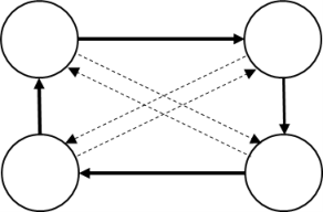
In this section, we present some numerical results to validate our theoretical findings on strongly connected digraphs with N=50N=50 nodes constructed by the following procedure: a directed ring links all the nodes, to ensure strong connectivity (cf. Fig. 3). Then directed edges are randomly added, with probability 0.20.2 on each pair of nodes.

VI-A Quantized weight-balancing

We adopt (13) for {γ⁡(k)}k∈ℤ+\{\gamma(k)\}_{k\in\mathbb{Z}_{+}}. We compare the total imbalance ‖𝐛⁡(k)‖1\|{\bf b}(k)\|_{1} of our proposed scheme with the integer weight-balancing and real weight-balancing schemes in [8]. The real weight-balancing scheme uses real valued communications; the integer weight-balancing scheme uses unicast transmissions to each of its out-neighbors to communicate the associated edge weight, and cannot use a prescribed number of bits. As we will see numerically, these features allow the scheme to converge to a weight-balanced solution within finite time. In contrast, our scheme uses broadcast communications with a prescribed number of bits per channel use, which in general does not guarantee convergence within finite time. The simulation results are averaged over 100 graph realizations.

Fig. 4 shows the total imbalance of Algorithm 1 with 1-bit and 5-bit of information exchange, as well as of the other two benchmark schemes. Note that in the integer weight-balancing scheme, the maximum weights in the 100 realizations are between 88 to 250, implying that 7 to 8 bits are required per edge per timeslot, which implies 77 or 8×(1+0.2×49)=75.68\times(1+0.2\times 49)=75.6 or 86.486.4 bits per node per timeslot. It is shown that the metric ‖𝐛⁡(k)‖1\|{\bf b}(k)\|_{1} is non-increasing for the proposed schemes, which is consistent with our analytical results (cf. L.3). In addition, one can see that the curve of ‖𝐛⁡(k)‖1\|{\bf b}(k)\|_{1} can be partitioned into nearly flat and steep line segments, for both schemes. The rationale behind this behavior is that the total imbalance decreases only when decreasing events occur (steep line segments); in between, the imbalance may be transferred within the network, but without causing the total imbalance to decrease. Compared with the two benchmark schemes, it shows that the proposed scheme with 50 bits outperforms the real weight-balancing scheme [8], which requires infinite rate communications. On the other hand, The comparison between the proposed 7-bit scheme and the integer weight-balancing scheme shows that, initially, the proposed scheme has better performance. However, as noted earlier, the integer weight-balancing scheme later outperforms the proposed 7-bit scheme since it is guaranteed to converge to a weight-balanced solution in finite timeslots.

VI-B Quantized average consensus

We compare our proposed algorithm with the following state-of-the-art schemes: 1) Q-Push-Sum, where we straightforwardly apply the finite-bit probabilistic quantization to the original push-sum algorithm in [34], i.e., zi​(0)=si,ψi​(0)=1,∀i∈𝒱z_{i}(0){=}s_{i},\psi_{i}(0){=}1,\forall i{\in}\mathcal{V},

ψi​(k+1)\displaystyle\psi_{i}(k+1) =ψi​(k)+α⁡(k)​∑j∈𝒩i−ai​j​(k)​[𝒬⁡(ψj​(k))−𝒬⁡(ψi​(k))];\displaystyle=\psi_{i}(k)+\alpha(k)\!\!\sum\limits_{j\in\mathcal{N}_{i}^{-}}{\!\!\!a_{ij}(k)\,\left[\mathcal{Q}\left(\psi_{j}(k)\right)-\mathcal{Q}\left(\psi_{i}(k)\right)\right]};
zi​(k+1)\displaystyle z_{i}(k+1) =zi​(k)+α⁡(k)​∑j∈𝒩i−ai​j​(k)​[𝒬⁡(zj​(k))−𝒬⁡(zi​(k))];\displaystyle=z_{i}(k)+\alpha(k)\!\!\sum\limits_{j\in\mathcal{N}_{i}^{-}}{\!\!\!a_{ij}(k)\,\left[\mathcal{Q}\left(z_{j}(k)\right)-\mathcal{Q}\left(z_{i}(k)\right)\right]};

and yi​(k)=zi​(k)ψi​(k)y_{i}(k)=\frac{z_{i}(k)}{\psi_{i}(k)} is the estimate of the initial average, where 𝒬⁡(∙)\mathcal{Q}\left(\bullet\right) is the quantization defined in (3); note that Q-Push-Sum can be regarded as the generalization of [27] to real valued initialization and finite rate communications; 2) Q-Run-Avg, where we apply the finite-bit probabilistic quantization to the algorithm in [30];55 5 Note: this algorithm requires 𝒪⁡(N)\mathcal{O}(N) memory space to store the estimate of the eigenvector of graph Laplacian at each node. 3) Q-Monte-Carlo, where we apply the BB-bit quantization

rβ​(x,B)=(1+β)max⁡{⌊log1+β⁡x⌋,2B}\displaystyle r_{\beta}(x;B)=(1+\beta)^{\max\left\{\lfloor\log_{1+\beta}x\rfloor,2^{B}\right\}}

to the Monte-Carlo based algorithm in [29, Section 4]. In this algorithm nodes exchange quantized random values sampled from the exponential distribution with parameter related to their current states. Note that exact convergence can be achieved by [30, 29] using infinite-bit quantized communications, [34] using real value communications, and [27] using integer value communications. However, there is no theoretical guarantee for all these benchmark schemes with finite bit quantization: our proposed scheme is the first algorithm solving the distributed average consensus over unbalanced digraphs with a prescribed finite rate communications.

We adopt the mean square error (MSE) MSE⁡(k)=V⁡(𝐲⁡(k))/N{\rm MSE}(k)=V({\bf y}(k))/N as defined in (35) as performance metric. The simulation results are averaged over 100 graph realizations and 100 initial value realizations, i.e., totally 10000 realizations.

For the proposed algorithm, we adopt: qmin=0,qmax=1q_{\min}{=}0,q_{\max}{=}1, Bi(w)​(k)=Bi(c)​(k)=50,∀i,∀kB_{i}^{\rm(w)}(k){=}B_{i}^{\rm(c)}(k){=}50,\forall i,\forall k; (13) is adopted for {γ⁡(k)}k∈ℤ+\{\gamma(k)\}_{k\in\mathbb{Z}_{+}}, and α⁡(k)=(k+1)−1,∀k∈ℤ+\alpha(k){=}(k+1)^{-1},\forall k{\in}\mathbb{Z}_{+}, which satisfies A.5; for Q-Push-Sum we use 50 bits and qmin=0,qmax=Nq_{\min}{=}0,q_{\max}{=}N to quantize ψ\psi, and 50 bits and qmin=0,qmax=1q_{\min}{=}0,q_{\max}{=}1 to quantize zz; for Q-Run-Avg we quantize each element of 𝐳∈ℝN{\bf z}\in{\mathbb{R}}^{N} (the estimate of the left eigenvector at 0 of graph Laplacian constructed by a row stochastic weight matrix) using 4 bits (i.e., totally 4×N=804{\times}N{=}80 bits required for quantizing 𝐳\bf z) and qmin=0,qmax=Nκq_{\min}{=}0,q_{\max}{=}N^{\kappa} with κ=1.15\kappa{=}1.15, and yy is quantized using 20 bits and qmin=0,qmax=1q_{\min}{=}0,q_{\max}{=}1; for Q-Monte-Carlo, we use 50 bits to quantize both XX and YY, and other parameters are: a=0,b=1,ε=10−3a{=}0,b{=}1,\varepsilon{=}10^{-3}. Note that the communication resource budget per node per timeslot is 100 bits in all schemes.
Refer to caption
Fig. 3: Illustration of the random graph model for N=4N=4, where dashed arrows represent potential directed links depending on the realizations.

Fig. 5 shows the MSE performance of Algorithm 2 as well as other benchmark schemes. It is shown that only the proposed scheme and the Q-Monte-Carlo are reaching the average consensus, among all finite rate schemes. Note that Q-Run-Avg and Q-Push-Sum seem also converge for some realizations, cf. Fig. 6. However, only the proposed scheme has theoretical convergence guarantees.

Fig. 7 shows the communication cost (left y-axis) and delay (right y-axis) needed by Algorithm 2 to reach a target MSE of 1×10⁻³¹\times 10^{-3} and 5×10⁻³⁵\times 10^{-3}, versus the total number of bits per channel use. The communication cost is defined as the product of the total number of bits per node per timeslot and the number of timeslots. For each parameter setting, we run 50 graph realizations and 10 initial value realizations. To avoid the average results affected by the outliers, we select the best 95%95\% of results to perform averaging. We observe that increasing the total number of bits reduces the number of timeslots required. On the other hand, there exists an optimal number of bits that minimizes the communication cost. Using more bits does not appear to be beneficial, since the communication cost becomes larger, and it is only marginally compensated by the reduction of the number of timeslots required.

Refer to caption
Fig. 4: Quantized weight-balancing problem: Total imbalance ‖𝐛⁡(k)‖1\|{\bf b}(k)\|_{1} the propsoed algorithm with 1-bit , 7-bit, and 50-bit, as well as the integer and real weight-balancing schemes [8].
Refer to caption
Fig. 5: Quantized average consensus problem: MSE of average consensus algorithms average over 10000 realizations.
Refer to caption
Fig. 6: Quantized average consensus problem: MSE of average consensus algorithms for a particular realization.
Refer to caption
Fig. 7: Quantized consensus problem: Communication cost (left y-axis, solid lines) and number of timeslots (right y-axis, dashed lines) needed to reach the target MSE, versus the total number of bits per channel use.

VII Conclusions

In this paper, we introduced a novel distributed algorithm that solves the weight-balancing problem using only quantized information and simplex communications. Building on this scheme, a second contribution of the paper was a novel distributed average consensus algorithm over non-balanced digraphs that uses quantized simplex communications. Convergence of the algorithm was proved using a novel line of analysis, based on a novel metric inspired by the positional system representation and a new step-size rule. Finally, numerical results validated our theoretical findings.

Appendix A Intermediate Results in the Proof of Theorem 2

A-A Preliminary definitions and results

Throughout the proof, we write the updates of Si+​(k),Si−​(k)S_{i}^{+}(k),S_{i}^{-}(k), bi​(k)b_{i}(k) of Algorithm 1 as

Si+​(k+1)\displaystyle S_{i}^{+}(k+1) ≜∑j=1Naj​i​(k+1)​=(5)​∑j∈𝒩i+[aj​i​(k)+γ⁡(k)​ni​(k)]\displaystyle\triangleq\sum\limits_{j=1}^{N}{a_{ji}(k+1)}\overset{\eqref{a_ij}}{=}\sum\limits_{j\in\mathcal{N}_{i}^{+}}{\left[a_{ji}(k)+\gamma(k)n_{i}(k)\right]}
=Si+​(k)+di+​γ​(k)​ni​(k),\displaystyle=S_{i}^{+}(k)+d_{i}^{+}\gamma(k)n_{i}(k), (43)
Si−​(k+1)\displaystyle S_{i}^{-}(k+1) ≜∑j=1Nai​j​(k+1)​=(5)​∑j∈𝒩i−[ai​j​(k)+γ⁡(k)​nj​(k)]\displaystyle\triangleq\sum\limits_{j=1}^{N}{a_{ij}(k+1)}\overset{\eqref{a_ij}}{=}\sum\limits_{j\in\mathcal{N}_{i}^{-}}{\left[a_{ij}(k)+\gamma(k)n_{j}(k)\right]}
=Si−​(k)+∑j∈𝒩i−γ⁡(k)​nj​(k),\displaystyle=S_{i}^{-}(k)+\sum\limits_{j\in\mathcal{N}_{i}^{-}}{\gamma(k)n_{j}(k)}, (44)
bi​(k+1)\displaystyle b_{i}(k+1) ≜Si−​(k+1)−Si+​(k+1)\displaystyle\triangleq S_{i}^{-}(k+1)-S_{i}^{+}(k+1)
=bi​(k)−di+​γ​(k)​ni​(k)+∑j∈𝒩i−γ⁡(k)​nj​(k).\displaystyle=b_{i}(k)-d_{i}^{+}\gamma(k)n_{i}(k)+\sum_{j\in\mathcal{N}_{i}^{-}}\!\!\!\gamma(k)n_{j}(k). (45)
Lemma 9.

Given 𝒱+​(k)\mathcal{V}^{+}(k) and 𝒱−​(k)\mathcal{V}^{-}(k), defined in (18), it holds:

ℐ⁡(𝒟k)=0⇒𝒱+​(k+1)⊇𝒱+​(k)​ and ​𝒱−​(k+1)⊇𝒱−​(k).\mathcal{I}(\mathcal{D}_{k}){=}0\,\,\Rightarrow\,\,\mathcal{V}^{+}(k+1){\supseteq}\mathcal{V}^{+}(k)\text{ and }\mathcal{V}^{-}(k+1){\supseteq}\mathcal{V}^{-}(k).
Proof:

Let ℐ​{𝒟k}=0\mathcal{I}\{\mathcal{D}_{k}\}{=}0 and consider i∈𝒱−​(k)i{\in}\mathcal{V}^{-}(k). Then, (4) and bi​(k)<0b_{i}(k){<}0 imply γ⁡(k)​ni​(k)>bi​(k)/di+\gamma(k)n_{i}(k){>}b_{i}(k)/d_{i}^{+}; ℐ​{𝒟k}=0\mathcal{I}\{\mathcal{D}_{k}\}{=}0 (see (14)) implies nj​(k)≤0,∀j∈𝒩i−n_{j}(k){\leq}0,\forall j{\in}\mathcal{N}_{i}^{-}. bi​(k+1)<0b_{i}(k{+}1){<}0 then follows from (45), so that i∈𝒱−​(k+1)i{\in}\mathcal{V}^{-}(k{+}1); hence 𝒱−​(k+1)⊇𝒱−​(k)\mathcal{V}^{-}(k{+}1){\supseteq}\mathcal{V}^{-}(k). 𝒱+​(k+1)⊇𝒱+​(k)\mathcal{V}^{+}(k{+}1){\supseteq}\mathcal{V}^{+}(k) follows from a similar argument on i∈𝒱+​(k)i{\in}\mathcal{V}^{+}(k). ∎

Lemma 10.

∀k∈ℤ+,∃τ≥k:‖𝐛⁡(τ)‖1<N2​γ​(τ)\forall{k}\in\mathbb{Z}_{+},\exists\tau\geq k:\|{\bf b}(\tau)\|_{1}<N^{2}\gamma(\tau).

Proof:

We prove it by contradiction. Let T¯0≜(2​W−1)​U¯\bar{T}_{0}\triangleq(2W-1)\bar{U}. Suppose ∃k∈ℤ+:‖𝐛⁡(τ)‖1≥N2​γ​(τ)\exists k\in\mathbb{Z}_{+}:\|{\bf b}(\tau)\|_{1}\geq N^{2}\gamma(\tau), for all τ≥k\tau\geq k. Invoking Corollary 5.(ii) recursively mm times and taking m→∞m\to\infty yields

0≤‖𝐛⁡(k+m​T¯0)‖1≤‖𝐛⁡(k)‖1−2​∑n=1mγ⁡(k+n​T¯0),\displaystyle 0\leq\left\|{\bf b}\big(k\!+\!m\,\bar{T}_{0}\big)\right\|_{1}\!\!\leq\!\left\|{\bf b}\big(k\big)\right\|_{1}\!\!-\!2\sum_{n=1}^{m}\!\gamma\big(k\!+\!n\,\bar{T}_{0}\big),

a contradiction since ∑n=1mγ⁡(k+n​T¯0)→∞\sum_{n=1}^{m}\gamma\left(k+n\bar{T}_{0}\right)\to\infty due to (12). ∎

A-B Proof of Lemma 6

By the definition of Cauchy sequence applied to each entry of 𝐀⁡(k){\bf A}(k), we need to prove that, ∀ϵ>0,∃kϵ∈ℤ+\forall\epsilon>0,\exists k_{\epsilon}\in\mathbb{Z}_{+} such that maxi,j⁡|ai​j​(m)−ai​j​(n)|<ϵ,∀m,n≥kϵ\max_{i,j}|a_{ij}(m)-a_{ij}(n)|<\epsilon,\forall m,n\geq k_{\epsilon}. To this end, let ϵ>0\epsilon{>}0 and define kϵk_{\epsilon} as66 6 Note that kϵ(i)<∞k_{\epsilon}^{(i)}<\infty since ‖𝐛⁡(k)‖1→0\|{\bf b}(k)\|_{1}\to 0 and γ⁡(k)→0\gamma(k)\to 0, see (12).

kϵ=min{k:∥𝐛(k)∥1<ϵ/(2U¯),ϵ/(4U¯)}.\displaystyle k_{\epsilon}=\min\{k:\|{\bf b}(k)\|_{1}<\epsilon/(2\bar{U}),\epsilon/(4\bar{U})\}. (46)

Since aj​i​(k)a_{ji}(k) is updated only at update or decreasing events, using (5) recursively, we infer

|aj​i​(k)−aj​i​(kϵ)|≤∑ℓ=kϵ∞ℐ⁡{𝒰ℓ∨𝒟ℓ}​γ​(ℓ),∀k≥kϵ.|a_{ji}(k)-a_{ji}(k_{\epsilon})|\leq\sum_{\ell=k_{\epsilon}}^{\infty}\mathcal{I}\{\mathcal{U}_{\ell}\vee\mathcal{D}_{\ell}\}\gamma(\ell),\ \forall k\geq k_{\epsilon}.

With tlt_{l} defined as in (15) and letting Lϵ≜min⁡{l∈ℤ+:tl≥kϵ}L_{\epsilon}\triangleq\min\{l\in\mathbb{Z}_{+}:t_{l}\geq k_{\epsilon}\}, we can further upper bound

|aj​i​(k)−aj​i​(kϵ)|≤\displaystyle|a_{ji}(k)-a_{ji}(k_{\epsilon})|\leq γ⁡(kϵ)​∑ℓ=kϵtLϵ−1ℐ⁡{𝒰ℓ∨𝒟ℓ}\displaystyle\gamma(k_{\epsilon})\sum_{\ell=k_{\epsilon}}^{t_{L_{\epsilon}}-1}\mathcal{I}\{\mathcal{U}_{\ell}\vee\mathcal{D}_{\ell}\} (47)
+∑l=Lϵ∞γ(tl)∑ℓ=tltl+1−1ℐ{𝒟ℓ∨𝒰ℓ}.\displaystyle+\sum_{l=L_{\epsilon}}^{\infty}\gamma(t_{l})\sum_{\ell=t_{l}}^{t_{l+1}-1}\mathcal{I}\{\mathcal{D}_{\ell}\vee\mathcal{U}_{\ell}\}.

Since there are at most U¯\bar{U} update events between the two consecutive decreasing events at times tlt_{l} and tl+1t_{l+1} (cf. C.5), it follows that ∑ℓ=tltl+1−1ℐ⁡{𝒟ℓ∨𝒰ℓ}≤U¯\sum_{\ell=t_{l}}^{t_{l+1}-1}\mathcal{I}\{\mathcal{D}_{\ell}\vee\mathcal{U}_{\ell}\}\leq\bar{U}, hence

|aj​i​(k)−aj​i​(kϵ)|≤[γ⁡(kϵ)+∑l=Lϵ∞γ⁡(tl)]​U¯.\displaystyle|a_{ji}(k)-a_{ji}(k_{\epsilon})|\leq\left[\gamma(k_{\epsilon})+\sum_{l=L_{\epsilon}}^{\infty}\gamma(t_{l})\right]\bar{U}. (48)

To bound ∑l=Lϵ∞γ⁡(tl)\sum_{l=L_{\epsilon}}^{\infty}\gamma(t_{l}), we apply recursively L.3,

−∥𝐛(kϵ)∥1=∑ℓ=kϵ∞[∥𝐛(ℓ+1)−∥𝐛(ℓ)∥1]\displaystyle-\|{\bf b}(k_{\epsilon})\|_{1}=\sum_{\ell=k_{\epsilon}}^{\infty}[\|{\bf b}(\ell+1)-\|{\bf b}(\ell)\|_{1}]
≤−2∑ℓ=kϵ∞γ(ℓ)ℐ{𝒟ℓ}=−2∑l=Lϵ∞γ(tl),\displaystyle\leq-2\sum_{\ell=k_{\epsilon}}^{\infty}\gamma(\ell)\mathcal{I}\{\mathcal{D}_{\ell}\}=-2\sum_{l=L_{\epsilon}}^{\infty}\gamma(t_{l}), (49)

hence ∑l=Lϵ∞γ⁡(tl)≤‖𝐛⁡(kϵ)‖1/2≤ϵ/(2​U¯)\sum_{l=L_{\epsilon}}^{\infty}\gamma(t_{l})\leq\|{\bf b}(k_{\epsilon})\|_{1}/2\leq\epsilon/(2\bar{U}). By combining (48) with (49) and (46), we finally obtain, ∀k≥kϵ\forall k\geq k_{\epsilon},

|aj​i​(k)−aj​i​(kϵ)|≤[γ⁡(kϵ)+‖𝐛⁡(kϵ)‖1/2]​U¯<ϵ/2,\displaystyle|a_{ji}(k)-a_{ji}(k_{\epsilon})|\leq\left[\gamma(k_{\epsilon})+\|{\bf b}(k_{\epsilon})\|_{1}/2\right]\bar{U}<\epsilon/2,

and, ∀n,m≥kϵ\forall n,m\geq k_{\epsilon},

|aj​i​(n)−aj​i​(m)|≤|aj​i​(n)−aj​i​(kϵ)|+|aj​i​(m)−aj​i​(kϵ)|<ϵ,\displaystyle|a_{ji}(n){-}a_{ji}(m)|\leq|a_{ji}(n){-}a_{ji}(k_{\epsilon})|+|a_{ji}(m)-a_{ji}(k_{\epsilon})|{<}\epsilon,

which proves that {𝐀⁡(k)}k∈ℤ+\{{\bf A}(k)\}_{k\in\mathbb{Z}_{+}} is a Cauchy sequence.

A-C Proof of Lemma 3

We first introduce the following intermediate result.

Lemma 11.

Let {𝐛⁡(k)}k∈ℤ+\{{\bf b}(k)\}_{k\in\mathbb{Z}_{+}} be the sequence generated by Algorithm 2. Then, bi​(k)/γ¯​(k)∈ℤ,∀i∈𝒱b_{i}(k)/\bar{\gamma}(k){\in}\mathbb{Z},\forall i\in\mathcal{V} and k∈ℤ+k\in\mathbb{Z}_{+}.

Proof:

We prove this lemma by induction using (45). The induction hypothesis holds at k=0k{=}0, since ai​j​(0)=1,∀(j,i)∈ℰa_{ij}(0){=}1,\forall(j,i)\in\mathcal{E} and γ¯​(0)=21−Bmax\bar{\gamma}(0){=}2^{1-B_{\max}} (cf. A.2). Suppose that it holds at k≥0k{\geq}0, i.e., bi​(k)/γ¯​(k)∈ℤ,∀ib_{i}(k)/\bar{\gamma}(k){\in}\mathbb{Z},\forall i. Then, since γ¯​(k+1)=γ¯​(k)/m⁡(k)\bar{\gamma}(k+1){=}\bar{\gamma}(k)/m(k), with m⁡(k)∈{1,c1}⊂ℤ+⁣+m(k){\in}\{1,c_{1}\}{\subset}\mathbb{Z}_{++} (A.2), it follows that bi​(k)/γ¯​(k+1)=m⁡(k)​bi​(k)/γ¯​(k)∈ℤb_{i}(k)/\bar{\gamma}(k+1)=m(k)b_{i}(k)/\bar{\gamma}(k){\in}\mathbb{Z} and γ⁡(k)​ni​(k)/γ¯​(k+1)=m⁡(k)​ni​(k)​2Bmax−1∈ℤ\gamma(k)n_{i}(k)/\bar{\gamma}(k+1)=m(k)n_{i}(k)2^{B_{\max}-1}{\in}\mathbb{Z}. Therefore, by (45), one can infer that bi​(k+1)/γ¯​(k+1)∈ℤb_{i}(k+1)/\bar{\gamma}(k+1)\in\mathbb{Z}, proving the induction step and completing the proof. ∎

Proof of Lemma 3: Let i∈𝒱i\in\mathcal{V} and k∈ℤ+k\in\mathbb{Z}_{+}. Using (45), we find

|bi​(k+1)|γ⁡(k)=|bi​(k)γ⁡(k)−di+​ni​(k)+∑j∈𝒩i−nj​(k)|.\displaystyle\frac{|b_{i}(k+1)|}{\gamma(k)}=\left|\frac{b_{i}(k)}{\gamma(k)}-d_{i}^{+}n_{i}(k)+\sum_{j\in\mathcal{N}_{i}^{-}}n_{j}(k)\right|. (50)

It will be useful to note that, as can be seen from (4), bi​(k)b_{i}(k), ni​(k)n_{i}(k) (possibly, ni​(k)=0n_{i}(k)=0) and bi​(k)−di+​ni​(k)b_{i}(k)-d_{i}^{+}n_{i}(k) have the same signs, yielding the following inequality for all ii,

|bi​(k+1)|γ⁡(k)≤△|bi​(k)|γ⁡(k)−di+​|ni​(k)|+∑j∈𝒩i−|nj​(k)|,\displaystyle\frac{|b_{i}(k+1)|}{\gamma(k)}\stackrel{{\scriptstyle\triangle}}{{\leq}}\frac{|b_{i}(k)|}{\gamma(k)}-d_{i}^{+}|n_{i}(k)|+\sum_{j\in\mathcal{N}_{i}^{-}}|n_{j}(k)|, (51)

where △\triangle stands for the triangle inequality. We now distinguish the two cases ℐ​{𝒟k}=0\mathcal{I}\{\mathcal{D}_{k}\}{=}0 and ℐ​{𝒟k}=1\mathcal{I}\{\mathcal{D}_{k}\}{=}1. If ℐ​{𝒟k}=0\mathcal{I}\{\mathcal{D}_{k}\}=0, from the negation of 𝒟k\mathcal{D}_{k} in (14) and from (4), it follows that bi​(k),ni​(k),bi​(k)−di+​ni​(k)b_{i}(k),n_{i}(k),b_{i}(k)-d_{i}^{+}n_{i}(k), and nj​(k),∀j∈𝒩i−n_{j}(k),\forall j\in\mathcal{N}_{i}^{-} have the same signs, so that (51) holds with equality, ∀i\forall i.

Conversely, if ℐ​{𝒟k}=1\mathcal{I}\{\mathcal{D}_{k}\}{=}1, there exists ℓ\ell and (j1,j2)∈[𝒩ℓ−]2(j_{1},j_{2}){\in}[\mathcal{N}_{\ell}^{-}]^{2} such that either 1) bℓ​(k)≠0b_{\ell}(k){\neq}0, nℓ​(k)≠0n_{\ell}(k){\neq}0 and sgn⁡(nj1​(k))=−sgn⁡(bℓ​(k)){\rm sgn}(n_{j_{1}}(k)){=}-{\rm sgn}(b_{\ell}(k)); or 2) bℓ​(k)=0b_{\ell}(k){=}0, nℓ​(k)=0n_{\ell}(k){=}0 and sgn⁡(nj1​(k))=−sgn⁡(nj2​(k)){\rm sgn}(n_{j_{1}}(k)){=}-{\rm sgn}(n_{j_{2}}(k)). In the first case (bℓ​(k)≠0b_{\ell}(k)\neq 0, nℓ​(k)≠0n_{\ell}(k)\neq 0 and sgn⁡(nj1​(k))=−sgn⁡(bℓ​(k)){\rm sgn}(n_{j_{1}}(k))=-{\rm sgn}(b_{\ell}(k))), we bound (50) as

|bℓ​(k+1)|γ⁡(k)≤△|bℓ​(k)γ⁡(k)−dℓ+​nℓ​(k)+nj1​(k)|+∑j∈𝒩ℓ−,j≠j1|nj​(k)|\displaystyle\frac{|b_{\ell}(k+1)|}{\gamma(k)}\stackrel{{\scriptstyle\triangle}}{{\leq}}\left|\frac{b_{\ell}(k)}{\gamma(k)}-d_{\ell}^{+}n_{\ell}(k)+n_{j_{1}}(k)\right|+\!\!\!\!\!\!\!\!\!\sum_{j\in\mathcal{N}_{\ell}^{-},j\neq j_{1}}\!\!\!\!\!|n_{j}(k)|
≤||bℓ​(k)|γ⁡(k)−dℓ+​|nℓ​(k)|−|nj1​(k)||+∑j∈𝒩ℓ−,j≠j1|nj​(k)|\displaystyle{\leq}\left|\frac{|b_{\ell}(k)|}{\gamma(k)}{-}d_{\ell}^{+}|n_{\ell}(k)|-|n_{j_{1}}(k)|\right|+\sum_{j\in\mathcal{N}_{\ell}^{-},j\neq j_{1}}|n_{j}(k)|
=|bℓ​(k)|γ⁡(k)−dℓ+​|nℓ​(k)|−2​min⁡{|nj1​(k)|,|bℓ​(k)|γ⁡(k)−dℓ+​|nℓ​(k)|}\displaystyle{=}\frac{|b_{\ell}(k)|}{\gamma(k)}{-}d_{\ell}^{+}|n_{\ell}(k)|-2\min\left\{|n_{j_{1}}(k)|,\frac{|b_{\ell}(k)|}{\gamma(k)}{-}d_{\ell}^{+}|n_{\ell}(k)|\right\}
+∑j∈𝒩ℓ−|nj(k)|.\displaystyle\quad+\sum_{j\in\mathcal{N}_{\ell}^{-}}|n_{j}(k)|.

In the second case (bℓ​(k)=0b_{\ell}(k){=}0, nℓ​(k)=0n_{\ell}(k){=}0, sgn⁡(nj1​(k))=−sgn⁡(nj2​(k)){\rm sgn}(n_{j_{1}}(k)){=}-{\rm sgn}(n_{j_{2}}(k)) and, without loss of generality, |nj1​(k)|≥|nj2​(k)|≥21−Bmax|n_{j_{1}}(k)|{\geq}|n_{j_{2}}(k)|\geq 2^{1-B_{\max}}), we bound instead

|bℓ​(k+1)|γ⁡(k)≤△|bℓ​(k)γ⁡(k)−dℓ+​nℓ​(k)|+|nj1​(k)+nj2​(k)|+∑j∈𝒩ℓ−,j≠j1,j2|nj​(k)|\displaystyle\frac{|b_{\ell}(k{+}1)|}{\gamma(k)}{\stackrel{{\scriptstyle\triangle}}{{\leq}}}\left|\frac{b_{\ell}(k)}{\gamma(k)}{-}d_{\ell}^{+}n_{\ell}(k)\right|+\Bigr|n_{j_{1}}(k){+}n_{j_{2}}(k)\Bigr|\!\!+\!\!\!\!\!\!\!\!\!\!\!\!\!\sum_{j\in\mathcal{N}_{\ell}^{-},j\neq j_{1},j_{2}}\!\!\!\!\!\!\!\!\!\!\!\!|n_{j}(k)|
≤|bℓ​(k)|γ⁡(k)−dℓ+​|nℓ​(k)|+∑j∈𝒩ℓ−|nj​(k)|−2​|nj2​(k)|.\displaystyle{\leq}\frac{|b_{\ell}(k)|}{\gamma(k)}-d_{\ell}^{+}|n_{\ell}(k)|+\sum_{j\in\mathcal{N}_{\ell}^{-}}|n_{j}(k)|-2|n_{j_{2}}(k)|. (52)

In both cases, since |nj2​(k)|≥21−Bmax|n_{j_{2}}(k)|{\geq}2^{1-B_{\max}}, |nj1​(k)|≥21−Bmax|n_{j_{1}}(k)|{\geq}2^{1-B_{\max}} and γ⁡(k)​|nℓ​(k)|≤|bℓ​(k)|/dℓ+\gamma(k)|n_{\ell}(k)|{\leq}|b_{\ell}(k)|/d_{\ell}^{+} (see (4)), we further bound

|bℓ​(k+1)|γ⁡(k)≤|bℓ​(k)|γ⁡(k)−dℓ+​|nℓ​(k)|+∑j∈𝒩ℓ−|nj​(k)|−22−Bmax.\displaystyle\!\!\!\!\!\frac{|b_{\ell}(k{+}1)|}{\gamma(k)}{\leq}\frac{|b_{\ell}(k)|}{\gamma(k)}{-}d_{\ell}^{+}|n_{\ell}(k)|{+}\sum_{j\in\mathcal{N}_{\ell}^{-}}|n_{j}(k)|{-}2^{2-B_{\max}}. (53)

By summing (51) (with strict equality if ℐ​{𝒟k}=0\mathcal{I}\{\mathcal{D}_{k}\}=0) and (53) over i∈𝒱i\in\mathcal{V}, it holds

‖𝐛⁡(k+1)‖1​{=‖𝐛⁡(k)‖1,if ​ℐ​{𝒟k}=0≤‖𝐛⁡(k)‖1−2​γ¯​(k),otherwise,\displaystyle\|{\bf b}(k+1)\|_{1}\begin{cases}=\|{\bf b}(k)\|_{1},&\text{if }\mathcal{I}\{\mathcal{D}_{k}\}=0\\ \leq\|{\bf b}(k)\|_{1}-2\bar{\gamma}(k),&\text{otherwise,}\end{cases}

after noticing that j∈𝒩i−⇔i∈𝒩j+j\in\mathcal{N}_{i}^{-}\Leftrightarrow i\in\mathcal{N}_{j}^{+}, hence

∑i,j∈𝒩i−|nj​(k)|=∑j,i∈𝒩j+|nj​(k)|=∑j=1N|nj​(k)|​dj+.\displaystyle\sum_{i,j\in\mathcal{N}_{i}^{-}}|n_{j}(k)|=\sum_{j,i\in\mathcal{N}_{j}^{+}}|n_{j}(k)|=\sum_{j=1}^{N}|n_{j}(k)|d_{j}^{+}.

This completes the proof.

A-D Proof of Proposition 4

Property (i): Note that U⁡(k)≥0U(k){\geq}0 since |bi​(k)|≥0|b_{i}(k)|{\geq}0, for all i∈𝒱i\in\mathcal{V}. To show that it is upper bounded, we use Uh≤U1,∀h≥1U_{h}{\leq}U_{1},\forall h{\geq}1 and ∪h𝒱h(k)⊆𝒱\cup_{h}\mathcal{V}_{h}(k)\subseteq\mathcal{V}, and write

U⁡(k)\displaystyle U(k) ≤∑h=1N−1Un​∑i∈𝒱h​(k)N≤U1​N​∑h=1N−1|𝒱h​(k)|≤N2​(N−1).\displaystyle\leq\sum\limits_{h=1}^{N-1}{U_{n}\sum\limits_{i\in\mathcal{V}_{h}(k)}{N}}\leq U_{1}N\sum\limits_{h=1}^{N-1}{|\mathcal{V}_{h}(k)|}\leq N^{2(N-1)}.

We prove that U⁡(k)U(k) is nondecreasing as by product of the proof of Property (ii), as given below.

Property (ii): Since γ¯​(k+1)≤γ¯​(k)\bar{\gamma}(k+1)\leq\bar{\gamma}(k), we can lower bound U⁡(k+1)U(k+1) as

U⁡(k+1)≥∑h=1N−1Uh​∑j∈𝒱h​(k+1)min⁡{|bj​(k+1)|γ¯​(k),N}.\displaystyle U(k+1){\geq}\sum\limits_{h=1}^{N-1}U_{h}\sum\limits_{j\in\mathcal{V}_{h}(k{+}1)}\min\left\{\frac{|b_{j}(k+1)|}{\bar{\gamma}(k)},N\right\}.

Case 1: ℐ⁡(𝒟k)=ℐ⁡(𝒰k)=0\mathcal{I}(\mathcal{D}_{k})=\mathcal{I}(\mathcal{U}_{k})=0. We have bj​(k+1)=bj​(k),∀jb_{j}(k+1)=b_{j}(k),\forall j and 𝒱h​(k+1)≜𝒱h​(k),∀n\mathcal{V}_{h}(k{+}1)\triangleq\mathcal{V}_{h}(k),\forall n, which implies U⁡(k+1)≥U⁡(k)U(k+1)\geq U(k). Case 2: ℐ⁡(𝒰k)=1\mathcal{I}(\mathcal{U}_{k})=1. From the discussion following (51), (51) holds with equality:

|bi​(k+1)|γ⁡(k)=△|bi​(k)|γ⁡(k)−di+​ni​(k)+∑j∈𝒩i−|nj​(k)|,∀i.\displaystyle\!\!\!\!\!\frac{|b_{i}(k+1)|}{\gamma(k)}\stackrel{{\scriptstyle\triangle}}{{=}}\frac{|b_{i}(k)|}{\gamma(k)}-d_{i}^{+}n_{i}(k)+\sum_{j\in\mathcal{N}_{i}^{-}}|n_{j}(k)|,\ \forall i. (54)

Moreover, ∃i∈𝒱:ni​(k)≠0\exists i\in\mathcal{V}:n_{i}(k)\neq 0; this implies that there exists a non-empty set of nodes that receive at least one update from their in-neighbors, defined as

ℛ(k)={i∈𝒱:nj(k)≠0,∃j∈𝒩i−}.\mathcal{R}(k)=\{i\in\mathcal{V}:n_{j}(k)\neq 0,\exists j\in\mathcal{N}_{i}^{-}\}.

It is straightforward to show that

ℛ⁡(k)⊆𝒱+​(k+1)∪𝒱−​(k+1).\displaystyle\mathcal{R}(k)\subseteq\mathcal{V}^{+}(k+1)\cup\mathcal{V}^{-}(k+1). (55)

In fact, if i∉𝒱+​(k+1)∪𝒱−​(k+1)i\notin\mathcal{V}^{+}(k+1)\cup\mathcal{V}^{-}(k+1) (i.e., bi​(k+1)=0b_{i}(k+1)=0), it follows that i∉𝒱+​(k)∪𝒱−​(k)i\notin\mathcal{V}^{+}(k)\cup\mathcal{V}^{-}(k) (i.e., bi​(k)=0b_{i}(k)=0 and ni​(k)=0n_{i}(k)=0, cf. L.9); therefore, setting bi​(k+1)=bi​(k)=0b_{i}(k+1)=b_{i}(k)=0 and ni​(k)=0n_{i}(k)=0 in (54), we find that nj​(k)=0,∀j∈𝒩i−n_{j}(k)=0,\ \forall j\in\mathcal{N}_{i}^{-}, so that i∉ℛ⁡(k)i\notin\mathcal{R}(k) and (55) follows. With this definition, let

h∗=min⁡{h∈{1,2,…,N−1}:|𝒱h​(k+1)∩ℛ⁡(k)|>1}h^{*}=\min\{h\in\{1,2,\dots,N-1\}:|\mathcal{V}_{h}(k+1)\cap\mathcal{R}(k)|>1\}

be the distance of the node closest to those of opposite sign of balance at k+1k+1 to receive the update, and let ℓ∈𝒱h∗​(k+1)∩ℛ⁡(k)\ell\in\mathcal{V}_{h^{*}}(k+1)\cap\mathcal{R}(k) be one of such nodes. Then, we have

ni​(k)=0,∀i∈𝒱h​(k+1),∀h≤h∗.\displaystyle n_{i}(k)=0,\ \forall i\in\mathcal{V}_{h}(k+1),\,\,\forall h\leq h^{*}. (56)

In fact, if ni​(k)≠0n_{i}(k)\neq 0 for some of such ii, then ∃j∈𝒩i+∩𝒱h−1​(k+1)∩ℛ⁡(k)\exists j\in\mathcal{N}_{i}^{+}\cap\mathcal{V}_{h-1}(k+1)\cap\mathcal{R}(k) receiving the update, which contradicts the definition of h∗h^{*}. Reading (54) at i∈𝒱h​(k+1),h≤h∗i{\in}\mathcal{V}_{h}(k{+}1),h{\leq}h^{*}, yields

|bi​(k+1)|γ¯​(k)=|bi​(k)|γ¯​(k)+∑j∈𝒩i−|nj​(k)|21−Bmax≥|bi​(k)|γ¯​(k)+ℐ{i∈ℛ(k)}.\displaystyle\frac{|b_{i}(k+1)|}{\bar{\gamma}(k)}{=}\frac{|b_{i}(k)|}{\bar{\gamma}(k)}{+}\sum_{j\in\mathcal{N}_{i}^{-}}\frac{|n_{j}(k)|}{2^{1-B_{\max}}}{\geq}\frac{|b_{i}(k)|}{\bar{\gamma}(k)}{+}\mathcal{I}\{i{\in}\mathcal{R}(k)\}.

We can then further lower bound U⁡(k+1)U(k+1) as

U⁡(k+1)≥\displaystyle U(k{+}1){\geq} ∑h=1h∗Uh∑j∈𝒱h​(k+1)min{|bj​(k)|γ¯​(k),N}ℐ{(h,j)≠(h∗,ℓ)}\displaystyle\sum\limits_{h=1}^{h^{*}}U_{h}\!\!\!\!\!\!\!\sum\limits_{j\in\mathcal{V}_{h}(k{+}1)}\!\!\!\!\!\!\!\min\left\{\frac{|b_{j}(k)|}{\bar{\gamma}(k)},N\right\}\mathcal{I}\{(h,j){\neq}(h^{*},\ell)\}
+Uh∗​min⁡{|bi​(k)|γ¯​(k)+1,N},\displaystyle+U_{h^{*}}\min\left\{\frac{|b_{i}(k)|}{\bar{\gamma}(k)}+1,N\right\}, (57)

where we neglected the non-negative terms associated to 𝒱h​(k+1),h>h∗\mathcal{V}_{h}(k+1),h>h^{*}. To further bound this quantity, note that nℓ​(k)=0n_{\ell}(k)=0 (cf. (56)), which, together with Bi(w)​(k)>0,∀iB_{i}^{\rm(w)}(k)>0,\forall i for an update event to occur, implies bℓ​(k)/γ¯​(k)≤di+≤N−1b_{\ell}(k)/\bar{\gamma}(k)\leq d_{i}^{+}\leq N-1 (cf. (4)). Therefore min⁡{|bℓ​(k)|/γ¯​(k)+1,N}=min⁡{|bℓ​(k)|/γ¯​(k),N}+1\min\left\{|b_{\ell}(k)|/\bar{\gamma}(k)+1,N\right\}=\min\left\{|b_{\ell}(k)|/\bar{\gamma}(k),N\right\}+1. Finally, we use the fact that

0≥∑h=h∗+1N−1Uh​∑j∈𝒱h​(k+1)[min⁡{|bj​(k)|γ¯​(k),N}−N],0\geq\sum\limits_{h=h^{*}+1}^{N-1}U_{h}\sum\limits_{j\in\mathcal{V}_{h}(k+1)}\left[\min\left\{\frac{|b_{j}(k)|}{\bar{\gamma}(k)},N\right\}-N\right],

yielding

U⁡(k+1)≥\displaystyle U(k+1){\geq} ∑j∈𝒱min{|bj​(k)|γ¯​(k),N}∑h=1N−1Uhℐ{j∈𝒱h(k+1)}\displaystyle\sum\limits_{j\in\mathcal{V}}\min\left\{\frac{|b_{j}(k)|}{\bar{\gamma}(k)},N\right\}\sum\limits_{h=1}^{N-1}U_{h}\mathcal{I}\{j\in\mathcal{V}_{h}(k{+}1)\}
+Uh∗−N​∑h=h∗+1N−1Uh​|𝒱h​(k+1)|.\displaystyle+U_{h^{*}}-N\sum\limits_{h=h^{*}+1}^{N-1}U_{h}|\mathcal{V}_{h}(k+1)|. (58)

Now, using Uh≤Uh∗+1,∀h>h∗U_{h}{\leq}U_{h^{*}+1},\forall h{>}h^{*} and ∪h=h∗+1N−1𝒱h(k+1)⊆𝒱∖{ℓ}\cup_{h=h^{*}+1}^{N-1}\mathcal{V}_{h}(k{+}1)\subseteq\mathcal{V}\setminus\{\ell\}, we obtain

Uh∗−N​∑h=h∗+1N−1Uh​|𝒱h​(k+1)|\displaystyle U_{h^{*}}-N\sum\limits_{h=h^{*}+1}^{N-1}U_{h}|\mathcal{V}_{h}(k+1)| (59)
≥Uh∗−N​Uh∗+1​∑h=h∗+1N−1|𝒱h​(k+1)|≥N2​(N−h∗)−3≥N.\displaystyle\geq U_{h^{*}}-NU_{h^{*}+1}\sum\limits_{h=h^{*}+1}^{N-1}|\mathcal{V}_{h}(k+1)|\geq N^{2(N-h^{*})-3}\geq N.

In the last inequality, we used the fact that h∗≤N−2h^{*}{\leq}N-2. In fact, if h∗=N−1h^{*}{=}N{-}1, then (56) implies that ni​(k)=0,∀in_{i}(k){=0},\forall i, which contradicts the occurrence of the update event. Finally, note that 𝒱+​(k)⊆𝒱+​(k+1)\mathcal{V}^{+}(k){\subseteq}\mathcal{V}^{+}(k{+}1) and 𝒱−​(k)⊆𝒱−​(k+1)\mathcal{V}^{-}(k){\subseteq}\mathcal{V}^{-}(k{+}1) (cf. L.9), hence j∈𝒱h(k)⇒j∈∪m=1h𝒱m(k+1)j{\in}\mathcal{V}_{h}(k)\Rightarrow j{\in}\cup_{m=1}^{h}\mathcal{V}_{m}(k{+}1), i.e., jj gets closer to nodes of opposite sign. Together with Uh>Uh+1U_{h}{>}U_{h+1}, it implies

∑h=1N−1Uhℐ{j∈𝒱h(k+1)}≥∑h=1N−1Uhℐ{j∈𝒱h(k)}.\displaystyle\sum\limits_{h=1}^{N-1}U_{h}\mathcal{I}\{j\in\mathcal{V}_{h}(k{+}1)\}\geq\sum\limits_{h=1}^{N-1}U_{h}\mathcal{I}\{j\in\mathcal{V}_{h}(k)\}. (60)

The desired result follows by using (59)-(60) in (A-D).

Property (iii): We prove it by contradiction. Assume that t1,t2∈[k,tl+1)t_{1},t_{2}\in[k,t_{l+1}) such that 𝒰t1\mathcal{U}_{t_{1}} and 𝒰t2\mathcal{U}_{t_{2}} are two consecutive update events with t2−t1>2​W−1t_{2}-t_{1}>2W-1, and ‖𝐛⁡(t)‖1≥N2​γ​(t),∀t∈[k,tl+1)\|{\bf b}(t)\|_{1}\geq N^{2}\gamma(t),\forall t\in[k,t_{l+1}). It follows that ∃i∈𝒱\exists i\in\mathcal{V} such that

|bi​(t1)|≥N​γ​(t1)≥(A​.2)N​γ​(t)>di+​γ​(t),∀t∈[t1,t1+2​W−1],|b_{i}(t_{1})|\geq N\gamma(t_{1})\stackrel{{\scriptstyle(A.2)}}{{\geq}}N\gamma(t)>d_{i}^{+}\gamma(t),\forall t\in[t_{1},t_{1}+2W-1],

which implies that ∃t∈[t1,t1+2​W−1]:ℐ⁡{𝒰t}=1\exists t\in[t_{1},t_{1}+2W-1]:\mathcal{I}\{\mathcal{U}_{t}\}=1 due to A.1, which contradicts the assumption that 𝒰t1\mathcal{U}_{t_{1}} and 𝒰t2\mathcal{U}_{t_{2}} are two consecutive update events since t1+2​W−1<t2t_{1}+2W-1<t_{2}. Hence, it follows from property (ii) that

U⁡(k+2​W−1)≥U⁡(k)+N,\displaystyle U(k+2W-1)\geq U(k)+N,

which proves property (iii). ■\blacksquare

Appendix B Auxiliary Results for Theorem 7

Lemma 12.

Let {𝐲⁡(k)}k∈ℤ+\{{\bf y}(k)\}_{k\in\mathbb{Z}_{+}} be the sequence generated by Algorithm 2, in the setting of T.7. Then, it holds:

𝟏⊤​𝐲​(k)=𝟏⊤​𝐲​(0)\displaystyle{\bf 1}^{\top}{\bf y}(k)={\bf 1}^{\top}{\bf y}(0)
Proof:

From (34) and 𝐋+​(k)=𝐒+​(k)−𝐀⁡(k){\bf L}^{+}(k)={\bf S}^{+}(k)-{\bf A}(k), it follows

𝟏T​𝐲​(k+1)=𝟏T​𝐲​(k)−α⁡(k)​𝟏T​[𝐒+​(k)−𝐀⁡(k)]​𝐱​(k),\displaystyle\mathbf{1}^{T}{\bf y}(k+1){=}\mathbf{1}^{T}{\bf y}(k){-}\alpha(k)\mathbf{1}^{T}[{\bf S}^{+}(k){-}{\bf A}(k)]\mathbf{x}(k), (61)

so that the statement of the lemma readily follows after noticing that 𝟏T​𝐀​(k)=𝐒+​(k)\mathbf{1}^{T}{\bf A}(k)={\bf S}^{+}(k). ∎

Lemma 13.

Let {𝐲⁡(k)}k∈ℤ+\{{\bf y}(k)\}_{k\in\mathbb{Z}_{+}} be the sequence generated by Algorithm 2, in the setting of T.7. Then,

yi,min≤yi,min(k)≤yi​(k)≤yi,max(k)≤yi,max,∀k∈ℤ+,y_{i,\min}\leq y_{i,\min}^{(k)}\leq y_{i}(k)\leq y_{i,\max}^{(k)}\leq y_{i,\max},\ \forall k{\in}\mathbb{Z}_{+},

where yi,max≜limt→∞yi,max(t)<∞,yi,min≜limt→∞yi,min(t)>∞y_{i,\max}{\triangleq}\lim_{t\to\infty}y_{i,\max}^{(t)}{<}\infty,y_{i,\min}{\triangleq}\lim_{t\to\infty}y_{i,\min}^{(t)}{>}\infty, q∗≜max⁡{|qmin|,|qmax|}q^{*}{\triangleq}\max\{|q_{\min}|,|q_{\max}|\}, Smax≜supk∈ℤ+Si−​(k)<∞S_{\max}{\triangleq}\sup_{k\in\mathbb{Z}_{+}}S_{i}^{-}(k){<}\infty,

yi,max(k)≜max⁡{qmax,yi​(0)}+α⁡(0)​‖𝐛⁡(0)‖1​q∗\displaystyle y_{i,\max}^{(k)}\triangleq\max\{q_{\max},y_{i}(0)\}+\alpha(0)\|{\bf b}(0)\|_{1}q^{*}
+α⁡(0)​Smax​(qmax−qmin)+q∗​∑t=0k−1α⁡(t)​|bi​(t)|,\displaystyle+\alpha(0)S_{\max}\left(q_{\max}-q_{\min}\right)+q^{*}\sum_{t=0}^{k-1}{\alpha(t)|b_{i}(t)|}, (62)
yi,min(k)≜min⁡{qmin,yi​(0)}−α⁡(0)​‖𝐛⁡(0)‖1​q∗\displaystyle y_{i,\min}^{(k)}\triangleq\min\{q_{\min},y_{i}(0)\}-\alpha(0)\|{\bf b}(0)\|_{1}q^{*}
−α⁡(0)​Smax​(qmax−qmin)−q∗​∑t=0k−1α⁡(t)​|bi​(t)|.\displaystyle-\alpha(0)S_{\max}\left(q_{\max}-q_{\min}\right)-q^{*}\sum_{t=0}^{k-1}{\alpha(t)|b_{i}(t)|}. (63)
Proof:

We first show that |yi,max|,|yi,min|<∞|y_{i,\max}|,|y_{i,\min}|{<}\infty. From T.2, we know that 𝐀⁡(k){\bf A}(k) is bounded for all k∈ℤ+k{\in}\mathbb{Z}_{+}, which implies Si−​(k)≤Smax<∞S_{i}^{-}(k)\leq S_{\max}<\infty. On the other hand, since |bi​(t)|≤‖𝐛⁡(t)‖1=𝒪⁡(1t)|b_{i}(t)|{\leq}\|{\bf b}(t)\|_{1}{=}\mathcal{O}\left(\frac{1}{t}\right) and ∑t∈ℤ+α​(t)2<∞\sum_{t\in\mathbb{Z}_{+}}{\alpha(t)^{2}}{<}\infty, one can verify using Cauchy-Schwarz inequality that ∑t=0∞α⁡(t)​|bi​(t)|<∞\sum_{t=0}^{\infty}{\alpha(t)|b_{i}(t)|}{<}\infty and thus |yi,max|,|yi,min|<∞|y_{i,\max}|,|y_{i,\min}|{<}\infty. By inspection, it is also clear that yi,max(k)≤yi,maxy_{i,\max}^{(k)}\leq y_{i,\max} and yi,min(k)≥yi,min,∀ky_{i,\min}^{(k)}\geq y_{i,\min},\forall k. We now prove yi​(k)∈[yi,min(k),yi,max(k)]y_{i}(k){\in}[y_{i,\min}^{(k)},y_{i,\max}^{(k)}] by induction. Clearly, it for k=0k=0. Now, assume it holds for some k≥0k\geq 0, we prove that this implies yi​(k+1)∈[yi,min(k+1),yi,max(k+1)]y_{i}(k{+}1){\in}[y_{i,\min}^{(k{+}1)},y_{i,\max}^{(k{+}1)}] (induction step). We have:

  1. 1.

    If yi​(k)≤qmaxy_{i}(k)\leq q_{\max}, then

    yi​(k+1)=yi​(k)+α⁡(k)​bi​(k)​xi​(k)\displaystyle y_{i}(k+1)=y_{i}(k)+\alpha(k)b_{i}(k)x_{i}(k)
    +α(k)∑j∈𝒩i−ai​j(k)(xj(k)−xi(k))\displaystyle+\alpha(k)\sum\limits_{j\in\mathcal{N}_{i}^{-}}{a_{ij}(k)\Big(x_{j}(k)-x_{i}(k)\Big)}
    ≤qmax+α⁡(k)​|bi​(k)|​q∗+α⁡(k)​Si−​(k)​(qmax−qmin)\displaystyle\leq q_{\max}+\alpha(k)|b_{i}(k)|q^{*}+\alpha(k)S_{i}^{-}(k)\left(q_{\max}-q_{\min}\right)
    ≤max⁡{qmax,yi​(0)}+α⁡(0)​‖𝐛⁡(0)‖1​q∗\displaystyle{\leq}\max\{q_{\max},y_{i}(0)\}{+}\alpha(0)\|{\bf b}(0)\|_{1}q^{*}
    +α⁡(0)​Smax​(qmax−qmin)=yi,max(0)≤yi,max(k+1).\displaystyle{+}\alpha(0)S_{\max}\left(q_{\max}{-}q_{\min}\right)=y_{i,\max}^{(0)}\leq y_{i,\max}^{(k+1)}.
  2. 2.

    If yi​(k)>qmaxy_{i}(k)>q_{\max}, then xi​(k)=qmaxx_{i}(k)=q_{\max}, so that (10) yields

    yi​(k+1)\displaystyle y_{i}(k+1) ≤yi​(k)+α⁡(k)​bi​(k)​qmax\displaystyle\leq y_{i}(k)+\alpha(k)b_{i}(k)q_{\max}
    ≤yi,max(k)+α⁡(k)​|bi​(k)|​q∗=yi,max(k+1).\displaystyle\leq y_{i,\max}^{(k)}+\alpha(k)|b_{i}(k)|q^{*}=y_{i,\max}^{(k+1)}.
  3. 3.

    Similarly, if yi​(k)≥qminy_{i}(k)\geq q_{\min} then

    yi​(k+1)≥min⁡{qmin,yi​(0)}−α⁡(0)​‖𝐛⁡(0)‖1​q∗\displaystyle y_{i}(k{+}1){\geq}\min\{q_{\min},y_{i}(0)\}{-}\alpha(0)\|{\bf b}(0)\|_{1}q^{*}
    −α⁡(0)​Smax​(qmax−qmin)=yi,min(0)≥yi,min(k+1).\displaystyle{-}\alpha(0)S_{\max}\left(q_{\max}{-}q_{\min}\right)=y_{i,\min}^{(0)}\geq y_{i,\min}^{(k+1)}.
  4. 4.

    If yi​(k)<qminy_{i}(k)<q_{\min}, then xi​(k)=qminx_{i}(k)=q_{\min} so that (10) yields

    yi​(k+1)\displaystyle y_{i}(k+1) ≥yi​(k)−α⁡(k)​|bi​(k)|​q∗\displaystyle\geq y_{i}(k)-\alpha(k)|b_{i}(k)|q^{*}
    ≥yi,min(k)−α⁡(k)​|bi​(k)|​q∗=yi,min(k+1).\displaystyle\geq y_{i,\min}^{(k)}-\alpha(k)|b_{i}(k)|q^{*}=y_{i,\min}^{(k+1)}.

∎

Lemma 14.

Let {𝐲⁡(k)}k∈ℤ+\{{\bf y}(k)\}_{k\in\mathbb{Z}_{+}} be the sequence generated by Algorithm 2, in the setting of T.7. Then,

𝐲​(k)⊤​𝐋+​(k)​𝐲~​(k)≥ξ1​V​(𝐲⁡(k))−ξ2​‖𝐛⁡(k)‖1,\displaystyle{\bf y}(k)^{\top}{\bf L}^{+}(k)\tilde{\bf y}(k)\geq\xi_{1}V({\bf y}(k))-\xi_{2}\|{\bf b}(k)\|_{1}, (64)

for some finite constants ξ1,ξ2>0\xi_{1},\xi_{2}>0.

Proof:

Let 𝐞^​(k)=𝐲​(k)−𝐲~​(k)\hat{\bf e}(k){=}{\bf y}(k){-}\tilde{\bf y}(k) be the saturation error,
𝐒±​(k)=diag⁡{Si±​(k),∀i}{\bf S}^{\pm}\!(k){=}{\rm diag}\!\left\{\!S_{i}^{\pm}\!(k),\forall i\right\}, 𝐁⁡(k)=diag⁡{𝐛⁡(k)}=𝐒−​(k)−𝐒+​(k){\bf B}(k){=}{\rm diag}\!\left\{\!\mathbf{b}(k)\right\}{=}{\bf S}^{-}\!(k){-}{\bf S}^{+}\!(k),
𝐋±​(k)=𝐒±​(k)−𝐀⁡(k){\bf L}^{\pm}\!(k){=}{\bf S}^{\pm}\!(k){-}{\bf A}\!(k), 𝐋⁡(k)=[𝐒+​(k)+𝐒−​(k)]−[𝐀⁡(k)+𝐀​(k)⊤]{\bf L}(k){=}[{\bf S}^{+}\!(k){+}{\bf S}^{-}\!(k)]{-}[{\bf A}\!(k){+}{\bf A}\!(k)^{\top}]. The proof contains three steps:

  • •

    Step 1: We will lower bound 𝐲​(k)⊤​𝐋+​(k)​𝐲~​(k){\bf y}(k)^{\top}{\bf L}^{+}(k)\tilde{\bf y}(k) as

    𝐲​(k)⊤​𝐋+​(k)​𝐲~​(k)≥−𝐲​(k)⊤​𝐁​(k)​𝐲~​(k)\displaystyle{\bf y}(k)^{\top}{\bf L}^{+}(k)\tilde{\bf y}(k)\geq-{\bf y}(k)^{\top}{\bf B}(k)\tilde{\bf y}(k)
    +12​𝐲~​(k)⊤​𝐁​(k)​𝐲~​(k)+12​𝐲~​(k)⊤​𝐋​(k)​𝐲~​(k).\displaystyle+\frac{1}{2}\tilde{\bf y}(k)^{\top}{\bf B}(k)\tilde{\bf y}(k)+\frac{1}{2}\tilde{\bf y}(k)^{\top}{\bf L}(k)\tilde{\bf y}(k). (65)
  • •

    Step 2: we will show that the last term of the RHS in Step 1 satisfies, for some ξ4>0\xi_{4}>0,

    𝐲~​(k)⊤​𝐋​(k)​𝐲~​(k)≥ξ4​V​(𝐲⁡(k)).\displaystyle\tilde{\bf y}(k)^{\top}{\bf L}(k)\tilde{\bf y}(k)\geq\xi_{4}V({\bf y}(k)). (66)
  • •

    Step 3: by combining the above results, we will show that, for some constants ξ1,ξ2>0\xi_{1},\xi_{2}>0,

    𝐲​(k)⊤​𝐋+​(k)​𝐲~​(k)≥ξ1​V​(𝐲⁡(k))−ξ2​‖𝐛⁡(k)‖1.\displaystyle{\bf y}(k)^{\top}{\bf L}^{+}(k)\tilde{\bf y}(k)\geq\xi_{1}V({\bf y}(k))-\xi_{2}\|{\bf b}(k)\|_{1}.

In the following, we provide detailed derivations of each step.

  • •

    Step 1: It is easy to show that

    𝐲​(k)⊤​𝐋+​(k)​𝐲~​(k)=−𝐲​(k)⊤​𝐁​(k)​𝐲~​(k)+𝐲​(k)⊤​𝐋−​(k)​𝐲~​(k).\displaystyle\!\!\!\!\!\!{\bf y}(k)^{\top}{\bf L}^{+}(k)\tilde{\bf y}(k){=}{-}{\bf y}(k)^{\top}{\bf B}(k)\tilde{\bf y}(k){+}{\bf y}(k)^{\top}{\bf L}^{-}(k)\tilde{\bf y}(k).

    The term 𝐲⊤​(k)​𝐋−​(k)​𝐲~​(k){\bf y}^{\top}(k){\bf L}^{-}(k)\tilde{\bf y}(k) can be lower bounded as

    𝐲​(k)⊤​𝐋−​(k)​𝐲~​(k)=𝐞^​(k)⊤​𝐋−​(k)​𝐲~​(k)+𝐲~​(k)⊤​𝐋−​(k)​𝐲~​(k)\displaystyle\!\!{\bf y}(k)^{\top}{\bf L}^{-}(k)\tilde{\bf y}(k){=}\hat{\bf e}(k)^{\top}{\bf L}^{-}(k)\tilde{\bf y}(k){+}\tilde{\bf y}(k)^{\top}{\bf L}^{-}(k)\tilde{\bf y}(k)
    ≥(a)​𝐲~​(k)⊤​𝐋−​(k)​𝐲~​(k)=12​𝐲~​(k)⊤​[𝐋−​(k)+𝐋−​(k)⊤]​𝐲~​(k)\displaystyle\!\!\overset{(a)}{\geq}\tilde{\bf y}(k)^{\top}{\bf L}^{-}(k)\tilde{\bf y}(k){=}\frac{1}{2}\tilde{\bf y}(k)^{\top}\left[{\bf L}^{-}(k){+}{\bf L}^{-}(k)^{\top}\right]\tilde{\bf y}(k)
    =12​𝐲~​(k)⊤​𝐁​(k)​𝐲~​(k)+12​𝐲~​(k)⊤​𝐋​(k)​𝐲~​(k),\displaystyle\!\!=\frac{1}{2}\tilde{\bf y}(k)^{\top}{\bf B}(k)\tilde{\bf y}(k)+\frac{1}{2}\tilde{\bf y}(k)^{\top}{\bf L}(k)\tilde{\bf y}(k),

    where (a)(a) comes from the fact that

    𝐞^​(k)⊤​𝐋−​(k)​𝐲~​(k)=𝐞^​(k)⊤​[𝐒−​(k)−𝐀⁡(k)]​𝐲~​(k)\displaystyle\hat{\bf e}(k)^{\top}{\bf L}^{-}(k)\tilde{\bf y}(k)=\hat{\bf e}(k)^{\top}[{\bf S}^{-}(k)-{\bf A}(k)]\tilde{\bf y}(k)
    =∑i=1N[e^i​(k)​∑j=1Nai​j​(k)​(y~i​(k)−y~j​(k))]≥0,\displaystyle=\sum_{i=1}^{N}{\Big[\hat{e}_{i}(k)\sum_{j=1}^{N}{a_{ij}(k)\left(\tilde{y}_{i}(k)-\tilde{y}_{j}(k)\right)}\Big]}\geq 0,

    where the last inequality comes from the fact that (i) if yi​(k)∈[qmin,qmax]y_{i}(k)\in[q_{\min},q_{\max}], then e^i​(k)=0\hat{e}_{i}(k)=0; (ii) if yi​(k)>qmaxy_{i}(k)>q_{\max}, then e^i​(k)>0\hat{e}_{i}(k)>0 and y~i​(k)−y~j​(k)=qmax−y~j​(k)≥0,∀j∈𝒱\tilde{y}_{i}(k)-\tilde{y}_{j}(k)=q_{\max}-\tilde{y}_{j}(k)\geq 0,\forall j\in\mathcal{V}; and (iii) if yi​(k)<qminy_{i}(k)<q_{\min}, then e^i​(k)<0\hat{e}_{i}(k)<0 and y~i​(k)−y~j​(k)=qmin−y~j​(k)≤0,∀j∈𝒱\tilde{y}_{i}(k)-\tilde{y}_{j}(k)=q_{\min}-\tilde{y}_{j}(k)\leq 0,\forall j\in\mathcal{V}.

  • •

    Step 2: First, one can verify that

    𝐲~​(k)⊤​𝐋​(k)​𝐲~​(k)=12​∑i,j=1N[ai​j​(k)+aj​i​(k)]​[y~i​(k)−y~j​(k)]2.\displaystyle\tilde{\bf y}(k)^{\top}{\bf L}(k)\tilde{\bf y}(k){=}\frac{1}{2}\sum\limits_{i,j=1}^{N}{[a_{ij}(k){+}a_{ji}(k)]\left[\tilde{y}_{i}(k){-}\tilde{y}_{j}(k)\right]^{2}}.

    Let i∗∈arg⁡maxi​{yi​(k)}i^{*}{\in}\arg\max_{i}\{y_{i}(k)\}, j∗∈arg⁡mini​{yi​(k)}j^{*}{\in}\arg\min_{i}\{y_{i}(k)\}, j∗≠i∗j^{*}\neq i^{*}. Note that yi∗​(k)≥y¯​(0)≥yj∗​(k){y}_{i^{*}}(k)\geq\bar{y}(0)\geq{y}_{j^{*}}(k) to preserve the average (L.12). Since 𝒢\mathcal{G} is strongly connected, there exists a path from i∗i^{*} to j∗j^{*}. Let {i1,⋯,ip}\{i_{1},\cdots,i_{p}\} be the set of nodes in the shortest path from i∗i^{*} to j∗j^{*}, with i1=i∗,ip=j∗i_{1}{=}i^{*},i_{p}{=}j^{*} and in+1∈𝒩in+,∀n∈[1,p−1]i_{n+1}{\in}\mathcal{N}_{i_{n}}^{+},\forall n\in[1,p-1]. We have

    𝐲~​(k)⊤​𝐋​(k)​𝐲~​(k)=12​∑i,j=1N[ai​j​(k)+aj​i​(k)]​[y~i​(k)−y~j​(k)]2\displaystyle\tilde{\bf y}(k)^{\top}{\bf L}(k)\tilde{\bf y}(k){=}\frac{1}{2}\sum\limits_{i,j=1}^{N}{[a_{ij}(k){+}a_{ji}(k)]\left[\tilde{y}_{i}(k){-}\tilde{y}_{j}(k)\right]^{2}}
    ≥12​∑l=1p−1[ail​il+1​(k)+ail+1​il​(k)]​[y~il​(k)−y~il+1​(k)]2\displaystyle\geq\frac{1}{2}\sum\limits_{l=1}^{p-1}{[a_{i_{l}i_{l+1}}(k)+a_{i_{l+1}i_{l}}(k)]\left[\tilde{y}_{i_{l}}(k)-\tilde{y}_{i_{l+1}(k)}\right]^{2}}
    ≥(a)​amin2​∑l=1p−1[y~il​(k)−y~il+1​(k)]2\displaystyle\overset{(a)}{\geq}\frac{a_{\min}}{2}\sum\limits_{l=1}^{p-1}{\left[\tilde{y}_{i_{l}}(k)-\tilde{y}_{i_{l+1}(k)}\right]^{2}}
    ≥(b)​amin2​(p−1)​{∑l=1p−1[y~il​(k)−y~il+1​(k)]}2\displaystyle\overset{(b)}{\geq}\frac{a_{\min}}{2(p-1)}\Big\{\sum\limits_{l=1}^{p-1}\left[{\tilde{y}_{i_{l}}(k)-\tilde{y}_{i_{l+1}}(k)}\right]\Big\}^{2}
    ≥amin2​(N−1)​[y~i∗​(k)−y~j∗​(k)]2,\displaystyle\geq\frac{a_{\min}}{2(N-1)}\left[\tilde{y}_{i^{*}}(k)-\tilde{y}_{j^{*}}(k)\right]^{2}, (67)

    where (a)(a) follows from ail+1​il​(k)≥amin,∀l∈[1,p),∀k∈ℤ+a_{i_{l+1}i_{l}}(k)\geq a_{\min},\forall l\in[1,p),\forall k\in\mathbb{Z}_{+} (T.2(i​i​i)(iii)); (b)(b) comes from Cauchy-Schwarz inequality. To further bound this quantity, note that

    1N​V​(𝐲)=1N​∑i[yi​(k)−y¯​(0)]2\displaystyle\frac{1}{N}V(\mathbf{y})=\frac{1}{N}\sum_{i}[{y}_{i}(k)-\bar{y}(0)]^{2}
    ≤maxi∈{i∗,j∗}⁡[yi​(k)−y¯​(0)]2≤[yi∗​(k)−yj∗​(k)]2.\displaystyle\leq\max_{i\in\{i^{*},j^{*}\}}[{y}_{i}(k)-\bar{y}(0)]^{2}\leq[y_{i^{*}}(k)-y_{j^{*}}(k)]^{2}. (68)

    On the other hand, since the consensus algorithm preserves the average, it follows

    yi∗​(k)−y¯​(0)≤(N−1)​(y¯​(0)−yj∗​(k))\displaystyle y_{i^{*}}(k)-\bar{y}(0)\leq(N-1)(\bar{y}(0)-y_{j^{*}}(k)) (69)
    y¯​(0)−yj∗​(k)≤(N−1)​(yi∗​(k)−y¯​(0)),\displaystyle\bar{y}(0)-y_{j^{*}}(k)\leq(N-1)(y_{i^{*}}(k)-\bar{y}(0)), (70)

    so that the first inequality in (68) is upper bounded as

    1N​V​(𝐲)≤(N−1)2​mini∈{i∗,j∗}​[yi​(k)−y¯​(0)]2.\frac{1}{N}V(\mathbf{y})\leq(N-1)^{2}\min_{i\in\{i^{*},j^{*}\}}[{y}_{i}(k)-\bar{y}(0)]^{2}.

    Consider the following two cases:

    1. (i)

      yi​(k)∈[qmin,qmax],∀iy_{i}(k){\in}[q_{\min},q_{\max}],\forall i, so that y~i​(k)=yi​(k),∀i\tilde{y}_{i}(k){=}y_{i}(k),\forall i and

      y~i∗​(k)−y~j∗​(k)=yi∗​(k)−yj∗​(k)≥1N​V⁡(𝐲).\displaystyle\tilde{y}_{i^{*}}(k)-\tilde{y}_{j^{*}}(k)=y_{i^{*}}(k)-y_{j^{*}}(k)\geq\frac{1}{\sqrt{N}}\sqrt{V(\mathbf{y})}.
    2. (ii)

      yi∗​(k)>qmaxy_{i^{*}}(k){>}q_{\max} (yj∗​(k)<qminy_{j^{*}}(k){<}q_{\min} can be solved similarly) so that y~i∗​(k)=qmax\tilde{y}_{i^{*}}(k){=}q_{\max}: since y~j∗​(k)≤max⁡{yj∗​(k),qmin}\tilde{y}_{j^{*}}(k){\leq}\max\{y_{j^{*}}(k),q_{\min}\}, using (69) and y¯​(0)≤qmax\bar{y}(0)\leq q_{\max} it follows

      y~i∗​(k)−y~j∗​(k)≥min⁡{yi∗​(k)−y¯​(0)N−1,qmax−qmin}\displaystyle\tilde{y}_{i^{*}}(k)-\tilde{y}_{j^{*}}(k){\geq}\min\Big\{\frac{y_{i^{*}}(k)-\bar{y}(0)}{N-1},q_{\max}-q_{\min}\Big\}
      ≥min⁡{V⁡(𝐲)N​(N−1)2,qmax−qmin}.\displaystyle\geq\min\Big\{\frac{\sqrt{V(\mathbf{y})}}{\sqrt{N}(N-1)^{2}},q_{\max}-q_{\min}\Big\}. (71)

    From (i), (ii) and (67), there exists some ξ4>0\xi_{4}>0 such that

    𝐲~​(k)⊤​𝐋​(k)​𝐲~​(k)≥amin2​(N−1)​(y~i∗​(k)−y~j∗​(k))2\displaystyle\tilde{\bf y}(k)^{\top}{\bf L}(k)\tilde{\bf y}(k)\geq\frac{a_{\min}}{2(N-1)}\left(\tilde{y}_{i^{*}}(k)-\tilde{y}_{j^{*}}(k)\right)^{2}
    ≥amin/2(N−1)​min⁡{V⁡(𝐲⁡(k))N​(N−1)4,(qmax−qmin)2}≥ξ4​V​(𝐲⁡(k)),\displaystyle\!\!\!\!\!\!\geq\frac{a_{\min}/2}{(N{-}1)}\min\left\{\frac{V\left({\bf y}(k)\right)}{N(N{-}1)^{4}},(q_{\max}{-}q_{\min})^{2}\right\}{\geq}\xi_{4}V({\bf y}(k)),

    since yi​(k)y_{i}(k) and thus V⁡(𝐲⁡(k))V({\bf y}(k)) is bounded (L.13).

  • •

    Step 3: Let y∗=maxi⁡{max⁡{|yi,max|,|yi,min|}}y^{*}=\max_{i}\{\max\{|y_{i,\max}|,|y_{i,\min}|\}\}. By combining (65) and (66), we get

    𝐲​(k)⊤​𝐋+​(k)​𝐲~​(k)\displaystyle\!\!\!\!{\bf y}(k)^{\top}{\bf L}^{+}(k)\tilde{\bf y}(k)
    ≥−𝐲​(k)⊤​𝐁​(k)​𝐲~​(k)+12​𝐲~​(k)⊤​𝐁​(k)​𝐲~​(k)+ξ1​V​(𝐲⁡(k))\displaystyle\!\!\!\!\!\!\geq-{\bf y}(k)^{\top}{\bf B}(k)\tilde{\bf y}(k)+\frac{1}{2}\tilde{\bf y}(k)^{\top}{\bf B}(k)\tilde{\bf y}(k)+\xi_{1}V({\bf y}(k))
    ≥−∑i=1N|bi(k)yi(k)y~i(k)|−12∑i=1N|bi(k)y~i(k)2|+ξ1V(𝐲(k))\displaystyle\!\!\!\!\!\!\geq\!{-}\!\sum_{i=1}^{N}{|b_{i}(k)y_{i}(k)\tilde{y}_{i}(k)|}{-}\frac{1}{2}\!\sum_{i=1}^{N}{|b_{i}(k)\tilde{y}_{i}(k)^{2}|}{+}\xi_{1}V({\bf y}(k))
    ≥(a)−q∗​(y∗+12​q∗)​‖𝐛⁡(k)‖1+ξ1​V​(𝐲⁡(k)),\displaystyle\!\!\!\!\!\!\overset{(a)}{\geq}-q^{*}\left(y^{*}+\frac{1}{2}q^{*}\right)\|{\bf b}(k)\|_{1}+\xi_{1}V({\bf y}(k)),

    with ξ1=ξ4/2>0\xi_{1}{=}\xi_{4}/2{>}0, where (a)(a) comes from the facts |yi​(k)|≤y∗|y_{i}(k)|\leq y^{*}, |y~i​(k)|≤q∗|\tilde{y}_{i}(k)|\leq q^{*}, and ‖𝐛⁡(k)‖1=∑i=1N|bi​(k)|\|{\bf b}(k)\|_{1}=\sum_{i=1}^{N}{|b_{i}(k)|}.

∎

References

  • [1] C. Lee, N. Michelusi, and G. Scutari, “Distributed quantized weight-balancing and average consensus over digraphs,” in Proc. IEEE Conf. on Decis. and Control, Dec. 2018, pp. 5857–5862.
  • [2] P. D. Lorenzo and G. Scutari, “Next: In-network nonconvex optimization,” IEEE Trans. Signal Inf. Process. Netw., vol. 2, no. 2, pp. 120–136, Jun. 2016.
  • [3] C. N. Hadjicostis and A. D. Domínguez-García, “Distributed balancing of commodity networks under flow interval constraints,” IEEE Trans. Autom. Control, vol. 64, no. 1, pp. 51–65, Jan. 2019.
  • [4] R. Olfati-Saber and R. M. Murray, “Consensus problems in networks of agents with switching topology and time-delays,” IEEE Trans. Autom. Control, vol. 49, no. 9, pp. 1520–1533, Sep. 2004.
  • [5] G. Cybenko, “Dynamic load balancing for distributed memory multiprocessors,” J. Parallel and Distrib. Comput., vol. 7, no. 2, pp. 279–301, 1989.
  • [6] J. A. Fax and R. M. Murray, “Information flow and cooperative control of vehicle formations,” IEEE Trans. Autom. Control, vol. 49, no. 9, pp. 1465–1476, Sep. 2004.
  • [7] G. Scutari, S. Barbarossa, and L. Pescosolido, “Distributed decision through self-synchronizing sensor networks in the presence of propagation delays and asymmetric channels,” IEEE Trans. Signal Process., vol. 56, no. 4, pp. 1667–1684, Apr. 2008.
  • [8] A. I. Rikos, T. Charalambous, and C. N. Hadjicostis, “Distributed weight balancing over digraphs,” IEEE Trans. Control Netw. Syst., vol. 1, no. 2, pp. 190–201, Jun. 2014.
  • [9] L. Hooi-Tong, “On a class of directed graphs-with an application to traffic-flow problems,” Operations Res., vol. 18, no. 1, pp. 87–94, 1970.
  • [10] B. Gharesifard and J. Cortés, “Distributed strategies for generating weight-balanced and doubly stochastic digraphs,” Eur. J. of Control, vol. 18, no. 6, pp. 539 – 557, 2012.
  • [11] A. I. Rikos and C. N. Hadjicostis, “Distributed balancing with constrained integer weights,” IEEE Trans. Autom. Control, vol. 64, no. 6, pp. 2553–2558, Jun. 2019.
  • [12] ——, “Distributed integer weight balancing in the presence of time delays in directed graphs,” IEEE Trans. Control Netw. Syst., vol. 5, no. 3, pp. 1300–1309, Sep. 2018.
  • [13] A. Kashyap, T. Basar, and R. Srikant, “Quantized consensus,” Automatica, vol. 43, no. 7, pp. 1192–1203, May 2007.
  • [14] A. Nedic, A. Olshevsky, A. Ozdaglar, and J. N. Tsitsiklis, “On distributed averaging algorithms and quantization effects,” IEEE Trans. Autom. Control, vol. 54, no. 11, pp. 2506–2517, Oct. 2009.
  • [15] J. Lavaei and R. M. Murray, “Quantized consensus by means of gossip algorithm,” IEEE Trans. Autom. Control, vol. 57, no. 1, pp. 19–32, Jan. 2012.
  • [16] M. El Chamie, J. Liu, and T. Basar, “Design and analysis of distributed averaging with quantized communication,” IEEE Trans. Autom. Control, vol. 61, no. 12, pp. 3870–3884, Dec. 2016.
  • [17] S. Zhu and B. Chen, “Distributed average consensus with bounded quantization,” in Proc. IEEE 17th Int. Workshop on Signal Process. Advances in Wireless Commun., Jul. 2016, pp. 1–6.
  • [18] T. C. Aysal, M. J. Coates, and M. G. Rabbat, “Distributed average consensus with dithered quantization,” IEEE Trans. Signal Process., vol. 53, no. 10, pp. 4905–4918, Oct. 2008.
  • [19] S. Kar and J. M. F. Moura, “Distributed consensus algorithms in sensor networks: Quantized data and random link failures,” IEEE Trans. Signal Process., vol. 58, no. 3, pp. 1383–1400, Mar. 2010.
  • [20] T. Li, M. Fu, L. Xie, and J.-F. Zhang, “Distributed consensus with limited communication data rate,” IEEE Trans. Autom. Control, vol. 56, no. 2, pp. 279–292, Feb. 2011.
  • [21] D. Thanou, E. Kokiopoulou, Y. Pu, and P. Frossard, “Distributed average consensus with quantization refinement,” IEEE Trans. Signal Process., vol. 61, no. 1, pp. 194–205, Jan. 2013.
  • [22] R. Rajagopal and M. J. Wainwright, “Network-based consensus averaging with general noisy channels,” IEEE Trans. Signal Process., vol. 59, no. 1, pp. 373–385, Jan. 2011.
  • [23] H. Li, G. Chen, T. Huang, and Z. Dong, “High-performance consensus control in networked systems with limited bandwidth communication and time-varying directed topologies,” IEEE Trans. Neural Netw. Learn. Syst., vol. 28, no. 5, pp. 1043–1054, May 2017.
  • [24] C.-S. Lee, N. Michelusi, and G. Scutari, “Topology-agnostic average consensus in sensor networks with limited data rate,” in Proc. Asilomar Conf. Signals, Syst., Comput., Oct. 2017.
  • [25] Y. Wang, Q. Wu, and Y. Wang, “Quantized consensus with finite data rate under directed topologies,” in Proc. IEEE Conf. on Decis. and Control and Eur. Control Conf., Dec. 2011, pp. 6427–6432.
  • [26] Z. Chen, J. Ma, and X. Yu, “Consensus of general linear multi-agent systems under directed communication graph with limited data rate,” in Proc. 3rd Int. Symp. on Auton. Syst., May 2019, pp. 394–399.
  • [27] A. I. Rikos and C. N. Hadjicostis, “Distributed average consensus under quantized communication via event- triggered mass summation,” in Proc. IEEE Conf. on Decis. and Control, Dec. 2018, pp. 894–899.
  • [28] A. I. Rikos and C. N. Hadjicostis, “Distributed average consensus under quantized communication via event-triggered mass splitting,” Jul. 2019, arXiv:1907.10671v1.
  • [29] B. Charron-Bost and P. Lambein-Monette, “Randomization and quantization for average consensus,” in Proc. IEEE Conf. on Decis. and Control, Dec. 2018, pp. 3716–3721.
  • [30] S. Zhu, Y. C. Soh, and L. Xie, “Distributed parameter estimation with quantized communication via running average,” IEEE Trans. Signal Process., vol. 63, no. 17, pp. 4634–4646, Sep. 2015.
  • [31] J. N. Tsitsiklis, “Problems in decentralized decision making and computation,” Ph.D. dissertation, Mass. Inst. Technol., Cambridge, 1984.
  • [32] L. Xiao and S. Boyd, “Fast linear iterations for distributed averaging,” Syst. Control Lett., vol. 53, no. 1, pp. 65–78, 2004.
  • [33] L. Xiao, S. Boyd, and S. Lall, “A scheme for robust distributed sensor fusion based on average consensus,” in Proc. 4th Int. Symp. on Information Processing in Sensor Networks, Apr. 2005, pp. 63–70.
  • [34] D. Kempe, A. Dobra, and J. Gehrke, “Gossip-based computation of aggregate information,” in Proc. 44th Annu. IEEE Symp. on Found. of Comput. Sci., Oct. 2003, pp. 482–491.
  • [35] F. Blasa, S. Cafiero, G. Fortino, and G. Fatta, “Symmetric push-sum protocol for decentralised aggregation,” in Proc. Int. Conf. on Advances in P2P Syst., Jan. 2011, pp. 27–32.
  • [36] A. Olshevsky, I. C. Paschalidis, and A. Spiridonoff, “Fully asynchronous push-sum with growing intercommunication intervals,” in Proc. Annu. Amer. Control Conf., Jun. 2018, pp. 591–596.
  • [37] F. Fagnani and S. Zampieri, “Average consensus with packet drop communication,” SIAM J. on Control and Optim., vol. 48, no. 1, pp. 102–133, 2009.
  • [38] B. Gerencsér and J. M. Hendrickx, “Push-sum with transmission failures,” IEEE Trans. Autom. Control, vol. 64, no. 3, pp. 1019–1033, Mar. 2019.
  • [39] J. M. Hendrickx and J. N. Tsitsiklis, “Fundamental limitations for anonymous distributed systems with broadcast communications,” in Proc. 53rd Annu. Allerton Conf. on Commun., Control, and Comput., Sep. 2015, pp. 9–16.
  • [40] D. P. Bertsekas and J. N. Tsitsiklis, Parallel and Distributed Computation:Numerical Methods. Belmont, MA, USA: Athena Scientific, 1989.
  • [41] Z. Qu, Cooperative Control of Dynamical Systems: Applications to Autonomous Vehicles, 1st ed. Springer Publishing Company, Incorporated, 2009.
  • [42] S. Kar and J. M. F. Moura, “Distributed consensus algorithms in sensor networks with imperfect communication: Link failures and channel noise,” IEEE Trans. Inf. Theory, vol. 57, no. 1, pp. 355–369, Jan. 2009.
  • [43] R. Durrett, Probability: Theory and Examples, 4.1th ed. New York, NY, USA: Cambridge University Press (4th ed.), 2013.
[Uncaptioned image] Chang-Shen Lee received the B.Sc. degree in the electrical engineering and computer science honor program and the M.Sc. in communications engineering from National Chiao Tung University, Hsinchu, Taiwan, in 2012 and 2014, respectively. He joined the Department of Electrical and Computer Engineering, Purdue University, West Lafayette, IN, in 2016, where he is currently pursuing the Ph.D. degree. From 2015 to 2016, he was a Research Assistant with the Research Center for Information Technology Innovation, Academia Sinica, Taiwan. His research interests include distributed computing and optimization.
[Uncaptioned image] Nicolo Michelusi (S’09, M’13, SM’18) received the B.Sc. (with honors), M.Sc. (with honors) and Ph.D. degrees from the University of Padova, Italy, in 2006, 2009 and 2013, respectively, and the M.Sc. degree in Telecommunications Engineering from the Technical University of Denmark in 2009, as part of the T.I.M.E. double degree program. He was a post-doctoral research fellow at the Ming-Hsieh Department of Electrical Engineering, University of Southern California, USA, in 2013-2015. He is currently an Assistant Professor at the School of Electrical and Computer Engineering at Purdue University, IN, USA. His research interests lie in the areas of 5G wireless networks, millimeter-wave communications, stochastic optimization, distributed optimization. Dr. Michelusi serves as Associate Editor for the IEEE Transactions on Wireless Communications, and as a reviewer for several IEEE Transactions.
[Uncaptioned image] Gesualdo Scutari (S’05-M’06-SM’11) received the Electrical Engineering and Ph.D. degrees (both with honors) from the University of Rome “La Sapienza,” Rome, Italy, in 2001 and 2005, respectively. He is the Thomas and Jane Schmidt Rising Star Associate Professor with the School of Industrial Engineering, Purdue University, West Lafayette, IN, USA.He had previously held several research appointments, namely, at the University of California at Berkeley, Berkeley, CA, USA; Hong Kong University of Science and Technology, Hong Kong; and University of Illinois at Urbana-Champaign, Urbana, IL, USA. His research interests include continuous and distributed optimization, equilibrium programming, and their applications to signal processing and machine learning. He is a Senior Area Editor of the IEEE Transactions On Signal Processing and an Associate Editor of Siam J. on Optimization; he served as an Associate Editor of the IEEE Transactions on Signal and Information Processing over Networks; the IEEE Transactions on Signal Processing, and the IEEE Signal Processing Letters. He served on the IEEE Signal Processing Society Technical Committee on Signal Processing for Communications (SPCOM). He was the recipient of the 2006 Best Student Paper Award at the IEEE ICASSP 2006, the 2013 NSF CAREER Award, the 2015 Anna Maria Molteni Award for Mathematics and Physics, and the 2015 IEEE Signal Processing Society Young Author Best Paper Award.