Weights Adaptation Optimization of Heterogeneous Epidemic Spreading Networks: A Constrained Cooperative Coevolution StrategyYun Feng is with the Department of Systems Engineering and Engineering Management, City University of Hong Kong, Kowloon, Hong Kong, and also with the Central South University, Changsha, 410083, P. R. China. E-mail: yun.feng@my.cityu.edu.hk Bing-Chuan Wang is with the School of Automation, Central South University, Changsha, 410083, P. R. China. E-mail: wangbingchuancityu@gmail.com (Corresponding author: BC Wang)
Abstract
In this paper, the dynamic constrained optimization problem of weights adaptation for heterogeneous epidemic spreading networks is investigated. Due to the powerful ability of searching global optimum, evolutionary algorithms are employed as the optimizers. One major difficulty is that the dimension of the problem is increasing exponentially with the network size and most existing evolutionary algorithms cannot achieve satisfiable performance on large-scale optimization problems. To address this issue, a novel constrained cooperative coevolution () strategy, which can separate the original large-scale problem into different subcomponents, is employed to achieve the trade-off between the constraint and objective function.
Index Terms:
Evolutionary Computation, Constrained Optimization, Epidemic Spreading, Weights Adaptation.I Introduction
Epidemic spreading over complex networks [1] has attracted lots of attention since the pioneering work [2] of Daniel Bernoulli in 1760. Many researches have been focused on the mathematical modeling of disease spreading process, classical epidemic models such as the susceptible-infected-susceptible (SIS) [3, 4, 5, 6], and the susceptible-infected-recovered (SIR) [7] model have been well studied for decades. Since the spreading of disease (such as AIDS, SARS, etc.) may cause numerous damages to the human society, developing control policies for epidemic spreading process is of great significance, with potential applications in public health. As pointed out in [8], the two common strategies to suppress epidemic spreading scale are increasing the recovery rate and decreasing the infection rate. For example, in [9], the PID control laws were implemented for the classical SIR model where the vaccination rate is the control variable. Despite these innovative results, these studies did not take the “budget” or the so-called “control cost” into consideration, which must be taken into account in real-world scenarios. In recent years, optimal control of epidemic spreading [10, 11, 12, 13] has gained more and more attentions. For example, in [14], an optimal control strategy was designed for the vaccination, quarantine and treatment actions. For inhomogeneous epidemic dynamics, the optimal control problem was studied in [15].
Besides the above control strategies which are focusing on the epidemic spreading parameters, recently another control strategy which aims at adjusting topology of the underlying network was investigated [16]. Acting as the “bridge” for epidemic spreading from infected individuals to healthy ones, the network topology determines the epidemic transmission efficiency. A quantitative parameter that defines the strength of two nodes in a network is the value of weight between them. Since the physical meaning of the weight can be described by the contact frequency of two individuals, the intuitive idea of controlling the weights is more natural and practical than controlling the spreading parameters. In [17], an individual-based weight adaptation mechanism in which individuals’ contact strength is adaptable depending on the level of contagion spreading over the network was proposed. An optimal control formulation was also presented to address the trade-off between the global infected level and the local weight adaptation cost corresponding to the topology of the underlying contact network. In [16] and [17], the objective function contains both the infection cost and control cost. However, the problem of minimizing the infection cost with given fixed number of budget, i.e., the control cost, has not been studied, which is more practical than the unconstrained optimization problems. This motivates us to investigate the constrained optimization problem of weights adaptation.
Meanwhile, when solving the optimal control problems in both [16] and [17], the forward-backward sweep method (FBSM) [18] was used to find the numerical solutions, which is an indirect method itself. The intuitive idea of FBSM is that the initial value problem of the state equations is solved forward in time, using an estimate for the control and adjoint variables. Then the adjoint final value problem is solved backwards in time. These complicated procedures add several difficulties to the optimal problem, which can be summarized as follows:
- •
Need to compute various partial derivatives of the Hamiltonian and solve additional differential equations, which introduce more errors for the optimization problem.
- •
Need to make an initial guess of the adjoint variables, the sensitivity of the method to changes in initial guesses.
In [18], the authors found that the FBSM method fails to terminate under some circumstances.
Evolutionary algorithms (EAs) [19, 20] which are inspired by nature, have shown powerful searching ability for the global optimum with few restrictions. Also, since EAs are direct methods, the implementations are much simpler than other conventional methods. EAs have been widely used in the community of network science and engineering [21, 22, 23]. For example, a novel memetic algorithm which can preserve the community structure is proposed for the network embedding problem in [21]. As one of the most powerful evolutionary algorithm, differential evolution (DE) [24, 25, 26] has shown superior performance over other heuristic algorithms on very complex searching and optimization problems. The control parameters of DE are few and it is highly efficient [24]. This motivates us to solve the constrained optimization problem based on DE. However, since the weights adaptation involves all links in the network for a given period of time [17], the dimension of the optimal solution is relatively high. Solving this kind of large-scale optimization problem [27] is a challenging problem in the community of evolutionary computation. In addition, how to achieve the trade-off between the constraint and objective function is another difficulty.
Motivated by the above considerations, a dynamic constrained optimization problem of weights adaptation for heterogeneous epidemic spreading networks based on SIS model (In this manuscript, we only consider SIS model and SIR model will be studied in the future work) is formulated. To deal with the high-dimensional optimization problem, a novel constrained cooperative coevolution () strategy which can separate the original high-dimensional search space into some low-dimensional ones by random grouping strategy is proposed. The constraint-handling technique is employed to achieve the trade-off between the constraint and objective function. Moreover, as a commonly used variant of the classical DE, the differential evolution with neighborhood search (NSDE) [28] algorithm is employed as the optimizer for these sub-problems.
The main contributions of this paper can be summarized as follows:
- •
A dynamic constrained optimization problem of weights adaptation for heterogeneous epidemic spreading networks is formulated.
- •
Evolutionary computation techniques with strong searching ability as well as quite a small amount of demands are applied to solve this kind of problem.
- •
A novel constrained cooperative coevolution () strategy is tailored for this real-world large-scale optimization problem.
- •
It is easy to implement and the optimization process can be done once the basic network and epidemic parameters are given. For the feedback control strategy [29], information about the number of susceptible or infected individuals is needed for the control law updating while the proposed method does not require such information.
The proposed strategy has strong potentials to be applied to real-world scenarios for disease control. Actually the most widely and successfully used strategy in real-world, quarantine, is a special form of weights adaptation. In addition, the proposed strategy has no restrictions on the spreading network.
The rest of this paper is organized as follows. The model description and problem formulation are given in Section II. Differential evolution is briefly introduced in Section III. In Section IV, the methodology is given in detail. Some numerical experiments are presented in Section V. Finally, this paper is concluded in Section VI.
II Model Description and Problem formulation
II-A Heterogeneous Weighted SIS-based Network Model
In the heterogeneous weighted SIS-based network, all nodes can be classified into two possible states according to their health status, that is, susceptible and infected. Susceptible individuals can be infected by infected individuals through the links between them and in state . Meanwhile, infected individuals can be cured and become susceptible again and in state . To be more specific, every node at time is infected with probability Pr and susceptible with probability Pr. At each time , a node can only be in either of these two states, thus PrPr. The state for each individual at time is independent.
Then the following heterogeneous weighted SIS-based network model is obtained from the N-intertwined mean-field approximation (NIMFA) [30, 31, 17]:
| (1) |
where denotes the probability of node being infected at time . The infection and curing rates and for each node in the network are described by two independent Poisson processes; denotes the weight of edge from node to node ; is the number of nodes in the network.
Then (1) can be rewritten in the following compact form:
| (2) |
where and Here “” denotes a diagonal matrix.
To be noticed, the network considered here is a directed one and the weights of which are in association with the infected level in the network as it is shown in (2). Define for all node so that self-loop is not considered here.
II-B Problem Formulation
As it is shown in (2), the infected level can be controlled by the weights adaptation in the network. However, bearing the cost of weights adaptation in mind, a natural dynamic constrained optimization problem is formed as follows:
| (3) |
where is the set of all admissible weights; denotes the infection cost function for each individual , the objective function denotes the total infection cost for all individuals in the considered period ; denotes the cost function for weights adaptation and denotes the initial weight at , is a constant that characterizes the maximum cost of weight adaptation, is the inequality constraint.
The dynamic constrained optimization problem is interpreted as: how to design the adaptive weights for all links from to such that the infected level in the network can be suppressed to the maximally extent under given budgets.
III Differential Evolution
Differential evolution (DE) [32, 33] is used as a base optimizer to solve the dynamic constrained optimization problem in (3), which is arguably one of the most powerful stochastic real-parameter optimization algorithms in current use. Different from traditional EAs, DE uses difference of individual trial solutions to explore the objective function landscape. Typically, DE consists of four stages: initialization, mutation,
crossover, and selection.
Step 1: Initialization
The ultimate goal of DE is to find a global optimum point in a -dimensional real parameter space . In the beginning, a randomly initiated population which consists of (size of population) -dimensional individuals is generated. denotes the size of population where each individual with size denotes a solution that consists of the weighs of every directed link in the spreading network from time to time . The subsequent generations in DE are denoted by . The population at generation is denoted as follows:
where is the th target vector in current generation:
Initially (), the population should be uniformly randomized within the search space constrained by the maximum and minimum bounds: and . Hence the initialization is formulated as follows:
where is a uniformly distributed number between and .
Step 2: Mutation
The mutation operator aims to create a mutant vector for each target vector through utilizing the differential information of pairwise individuals. The following mutation operator is adopted in this paper.
DE/current-to-best/1:
where , is the mutant vector, and are mutually exclusive integers randomly chosen from , is the best individual in the current population, and the scaling factor is a positive control parameter for scaling the difference vectors.
Step 3: Crossover
The crossover operator is employed to enhance the diversity of the population. The trial vector is formed by exchanging components between the target vector and the mutant vector . The following binomial crossover is utilized:
| if | ||||
| otherwise. |
where , , is a randomly chosen index from . is the crossover rate.
Step 4: Selection
In the selection step, the target vector is compared with the trial vector , the better one can be survived in the next generation
| if | ||||
| otherwise. |
IV Methodology
IV-A Encoding Mechanism
As described above, the dimension of the decision space is related to the number of links in the network and the time length . To be more specific, for a directed network with nodes, we have
| (4) |
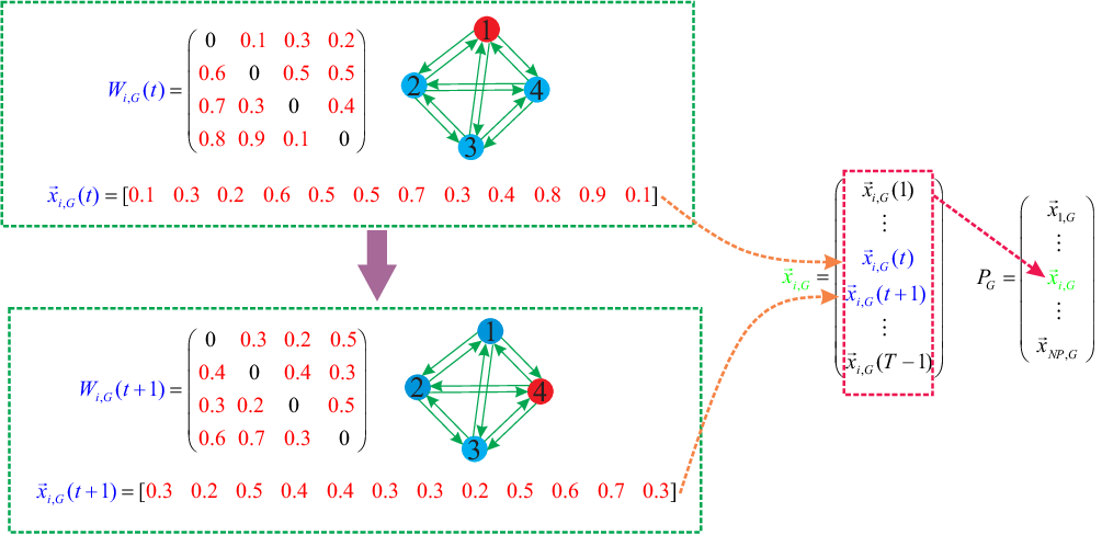
To better illustrate the encoding mechanism, a schematic graph is presented in Figure 1. The network consists of nodes, where blue and red nodes represent susceptible and infected individuals, respectively. denotes the th target vector in the -th generation, with a dimension of . Each element of corresponds to a specific element of the weight matrix at time in the manner presented in Figure 1. Bearing the infection cost and the weights adaption constraint in mind, the weight matrix at time is evolved adaptively to balance the objective function and constraint. Considering the time length , the th target vector at -th generation is formulated as:
To be noticed, the health status of all individuals in the network is varying from time to time. For example, as it is shown in Figure 1, node is infected at time while it is cured and become susceptible at time . Therefore, this is a dynamic optimization problem considering the interactions between the epidemic spreading process and weights adaptation.
Remark IV.1.
With this encoding mechanism, one inevitable problem is that the dimension of the decision space increases exponentially with the size of the network as it is shown in (4). Therefore, this constrained optimization problem (3) may suffers from the “curse of dimensionality”, which implies that most of the EAs’ performance deteriorates rapidly as the increasing of the dimensionality of the search space.
IV-B Differential Evolution with Neighborhood Search (NSDE)
As a variant of classical DE introduced in Section III, NSDE [28] is effective in escaping from local optima when searching in circumstances without knowing the preferred step size. The main difference between NSDE and DE is that the neighborhood search (NS) strategy is utilized, which is a typical technique in evolutionary programming (EP) [34]. To be more specific, the scaling factor in classical DE is replaced in the following manner:
| if | ||||
| otherwise. |
where is a Gaussian random number with mean 0.5 and standard deviation 0.5, and is a Cauchy random variable with scale parameter . In NSDE, the parameter was set to a constant number 0.5.
IV-C Constraint-handling Technique
The constraint-handling technique [35], which is adopted by the winner of IEEE CEC2010 competition, is utilized to compare two target vectors and . To be more specific, is better than if the following conditions are satisfied:
| if | (5a) | ||||
| if | (5b) | ||||
| otherwise. | (5c) |
where denotes the degree of constraint violation on the constraint as follows:
| if | ||||
| otherwise. |
where is the maximal degree of constraint violation of the initial population; is a parameter to truncate the value of ; is set to be in this paper.
IV-D A Constrained Cooperative Coevolution () Strategy
In this subsection, a novel coevolution strategy is developed to solve this dynamic constrained optimization problem motivated by the DECC-G algorithm in [27]. The core of this coevolution strategy is “divide-and-conquer”. That is, the original -dimensional search space is divided into number of -dimensional ones by random grouping strategy, where .
The constrained cooperative coevolution () framework for this problem can be summarized as follows:
(1) Set to start a new cycle.
(2) Decompose an original -dimensional target vector into low-dimensional subcomponents with dimension randomly, i.e. . Here “randomly” indicates that each dimension in the original target vector has the same probability to be assigned into any of the subcomponents.
(3) Optimize the th subcomponent with NSDE and constraint-handling technique introduced in Section IV-B and Section IV-C for a predefined number of fitness evaluations (FEs).
(4) if then and go to Step 3.
(5) Stop if halting criteria are satisfied; otherwise go to Step (1) for the next cycle.
Remark IV.2.
The probability of strategy to assign two interacting variables and into a single subcomponent for at least cycles is:
where is the total number of cycles and is the number of subcomponents.
In each separate cycle, the probability to assign two interacting variables and into a single subcomponent is
Let denotes the probability to assign and into a single subcomponent for exactly cycles. Obviously, satisfies the binomial distribution, so:
Thus,
Given network size and , then . Select , then the number of subcomponents . When the number of cycles , we have:
These results demonstrate that the strategy has relatively high probabilities to optimize interacting variables in a single subcomponent for at least one or two cycles.
IV-E NSDE under the framework
Considering NSDE as the base optimizer for the subcomponents, it is straightforward to obtain the NSDE with constrained cooperative coevolution algorithm, denoted as NSDE-. The pesudocode of NSDE- is given in Algorithm 1.
; 1
; 9
V Numerical Experiments
To validate the effectiveness of the proposed method, a synthetic network is obtained as the underlying network. When solving the dynamic constrained optimization problem in (3), each optimization algorithm is used for 25 independent runs.
V-A Datasets
For validation, one of the most famous synthetic complex network-the Bárabasi-Albert (BA) network [37] is used. When constructing the BA network, initially fully connected nodes are placed in the network. A new node is connected to existing nodes with probability proportional to the degree of them at each step [38]. A total number of nodes is fixed for the BA network in the simulations, originally this BA network is a bidirectional network.
The topologies of the BA network is presented in Figure 2, where circles represent nodes in the network and their sizes are proportional to degrees.
Table I below summarizes the topological features of the network, where denote the total number of nodes, average degree, average clustering coefficient and density of the network, respectively.
| Network name | ||||
|---|---|---|---|---|
| Bárabasi-Albert | 20 | 8.5 | 0.519 | 0.447 |
V-B Parameters Selection
For all experiments, the objective function for individual at time adopts the form:
Meanwhile, the cost function for weights adaptation for a pair of individuals and is:
The value of the constraint is selected as 700.
The objective function and the cost function adopt the current form for simple illustration. They represent one possible situation, there exists other sets of and in real-world scenarios. Since the weights adaptation optimization problem is still an open-problem and there lacks standard definition of both the objective function and the cost function, we adopted the current form similar to the way that was done in [16] and [17].
As for the value of the constraint , it was selected after the spreading network and epidemic parameters have been set.
Based on the underlying network introduced in the previous subsection, some numerical simulations are conducted to illustrate the effectiveness of the proposed method (NSDE-).
The epidemic parameters used in the simulations are presented in Table II, where denote the initial infection state, infection rate, curing rate, and terminal time, respectively. These parameters are carefully chosen to make sure that the infected level is relatively high when there is no weights adaptation, hence the effects of weights adaptation on epidemic spreading can be easily observed.
Remark V.1.
According to Theorem 2 in [39], assume that , then the metastable state is globally asymptotically stable when
where is the largest eigenvalue-the spectral radius of the matrix . Referring to the epidemic parameters in Table II, it is easily obtained that for the constructed BA network, hence the infected level is relatively high without weights adaptation.
Regarding to the algorithm parameters, the population size , the number of FEs and the crossover rate for both NSDE and NSDE- algorithms are the same. For NSDE- strategy, the dimension of the subcomponents is selected as .
| Network name | FEs | ||||||
|---|---|---|---|---|---|---|---|
| Bárabasi-Albert | 0.153 | 0.4 | 0.3 | 10 | 350 | 6.30e+06 | 0.9 |
V-C Results
For Bárabasi-Albert network, the simulation results are presented in Figure 3(a), 3(b), 3(c) and 3(d). Both the proposed NSDE- and the existing NSDE method are used. Meanwhile, two control groups are added for comparison, i.e. “No adaptation” and “constant adaptation” strategy. The formulation of these two strategies at time are as follows:
In this manner, these two strategies are employed as the baselines for comparison. “No adaptation” means that the weights remain unchanged in the considered time period, while “Constant adaptation” refers to a “discount” on the original weights with the budget fully used. For the epidemic parameters in Table II and , the constant adaptation ratio can be calculated as .
Figure 3(a) and 3(b) illustrate the evolution process of the mean best fitness value and constraint violation with respect to generations over 25 independent runs, respectively. For the “No adaptation” and “Constant adaptation” strategy, the solutions are determined initially. Hence the value of the objective function and constraint violation for these two strategies remain unchanged. For the “No adaptation” and “Constant adaptation” strategies, the constraint violation remains zero. Combing Figure 3(a) and 3(b), it is evident that the proposed NSDE- outperforms NSDE on BA network. Moreover, NSDE- outperforms both the “No adaptation” and “Constant adaptation” strategies.
Remark V.2.
One interesting phenomenon to be noticed in Figure 3(b) is that the evolution of constraint violation for NSDE- almost coincides with that of NSDE. However, the evolution of the mean best fitness value for these two algorithms are quite different. This is due to the use of constraint-handling technique in Section IV-C, which puts more emphasis on the constraint violation than the fitness value for earlier generations.
Figure 3(c) and 3(d) demonstrate the evolution process of two main indices, i.e. infected level and total weights over time, which characterize the epidemic spreading and weights adaptation level, respectively. The definition of theses two indices are as follows:
The physical meaning of the infected level and the total weights are the expectation of infection probability and total number of weights, respectively. In this manner, can be used as an index which reflects the current infected level among the whole population of individuals in the network. Similarly, reflects the weights variation of the network concerned. For infected level, “No adaptation” strategy achieves a relatively high level, which is used as a baseline for comparison as it is demonstrated in Section V-B and Remark V.1. However, the “Constant adaptation” strategy achieves a lower infected level than the “No adaptation” strategy, which is mainly due to that the “Constant adaptation” strategy makes full use of the budget as it is shown in Figure 3(d). Referring to the total weights variation in Figure 3(d), it is obvious that remains unchanged at every time for the “No adaptation” strategy. For the “Constant adaptation” strategy, the value of the total weights decreases to a lower value and keeps unchanged for the whole time period. However, for both the NSDE and NSDE- strategies, the value of total weights experience a decreasing process first and restore to the initial value of time , which coincide with the results in [17]. The restoring process of for NSDE- is more moderate than that of NSDE, hence the infected level is lower at most time. One interesting observation is that the value of the total weights for NSDE- drops to a lower value than that of the “Constant adaptation” strategy, and restores to the initial value at time , the infected levels indicate that this kind of “dynamically adaptation” is more effective in controlling the epidemic spreading scale.
In addition, to test statistical significance, the multi-problem Wilcoxon’s test [36] are implemented to compare these methods, the results are shown in Table III. Once more, the results indicate that the proposed NSDE- is superior to the other competitors.
| Algorithm | Mean OFV Std Dev | -value |
|---|---|---|
| NSDE- | 106.4530 0.1506 | - |
| NSDE | 127.1566 1.3425 | 1.4157e-09 |
| No adaptation | 160.5280 0.00 | 9.7285e-11 |
| Constant adaptation | 126.8617 0.00 | 9.7285e-11 |
Remark V.3.
To be noticed, the SIS model has been analytically and exactly solved in [40, 41], where the infection and recovery rate are time-varying. However, the NIMFA model is employed as the epidemic spreading model for its simplicity. In the future, we may extend our results with the help of the Lie algebra method.
VI Conclusion
In this paper, a dynamic constrained optimization problem of weights adaptation for heterogeneous epidemic spreading networks is formulated. Combining constrained cooperative coevolution () strategy with NSDE, a novel NSDE- algorithm is tailored for this problem. Numerical experiments on a BA network showed the effectiveness of this algorithm. In future research, how to expand this algorithm for on-line implementation is an interesting yet challenging topic. Moreover, the extension to the Mixed SI(R) epidemic dynamics in random graphs with general degree distributions and also the feedback control optimization are also our interests.
Some insights on the capability of our approach are provided as follows:
- •
First, in our problem setting, the dimension of a solution to be optimized increases exponentially with the increasing of the network size , which is obvious. And the curse of dimensionality problem is inevitable under such situations. However, even in the evolutionary computation community, state-of-the-art methods to deal with such large scale optimization problem is questionable. (The dimension of a solution in [27, 42] is only up to while it is in the numerical simulations studied in this manuscript.)
- •
The goal of this manuscript is not just to purse as high dimension as possible. More importantly, we focus on introducing evolutionary algorithms into the network optimization problems and shed some light on solving such large-scale optimization problems using the idea of cooperative coevolution.
In the numerical simulations, the number is selected due to the limitations on the hardware. Moreover, we do consider the capacity of the proposed algorithm seriously and there are still ways to improve. For example, for very large , we may consider dividing the solution of each subcomponent with dimension into small sub-subcomponents again and then deal with it in the same manner.
References
- [1] R. Pastor-Satorras, C. Castellano, P. Van Mieghem, and A. Vespignani, “Epidemic processes in complex networks,” Reviews of modern physics, vol. 87, no. 3, p. 925, 2015.
- [2] D. Bernoulli, “Essai d’une nouvelle analyse de la mortalité causée par la petite vérole, et des avantages de l’inoculation pour la prévenir,” Histoire de l’Acad., Roy. Sci.(Paris) avec Mem, pp. 1–45, 1760.
- [3] Y. Feng, Q. Fan, L. Ma, and L. Ding, “Epidemic spreading on uniform networks with two interacting diseases,” Physica A: Statistical Mechanics and its Applications, vol. 393, pp. 277–285, 2014.
- [4] B. Qu and H. Wang, “Sis epidemic spreading with heterogeneous infection rates,” IEEE Transactions on Network Science and Engineering, vol. 4, no. 3, pp. 177–186, 2017.
- [5] Y. Feng, L. Ding, Y.-H. Huang, and Z.-H. Guan, “Epidemic spreading on random surfer networks with infected avoidance strategy,” Chinese Physics B, vol. 25, no. 12, p. 128903, 2016.
- [6] Y. Huang, L. Ding, Y. Feng, and J. Pan, “Epidemic spreading in random walkers with heterogeneous interaction radius,” Journal of Statistical Mechanics: Theory and Experiment, vol. 2016, no. 10, p. 103501, 2016.
- [7] M. Nadini, A. Rizzo, and M. Porfiri, “Epidemic spreading in temporal and adaptive networks with static backbone,” IEEE Transactions on Network Science and Engineering, 2018.
- [8] C. Nowzari, V. M. Preciado, and G. J. Pappas, “Analysis and control of epidemics: A survey of spreading processes on complex networks,” IEEE Control Systems, vol. 36, no. 1, pp. 26–46, 2016.
- [9] L. L. Ghezzi and C. Piccardi, “Pid control of a chaotic system: An application to an epidemiological model,” Automatica, vol. 33, no. 2, pp. 181–191, 1997.
- [10] X.-J. Li, C. Li, and X. Li, “Minimizing social cost of vaccinating network sis epidemics,” IEEE Transactions on Network Science and Engineering, no. 1, pp. 1–1, 2017.
- [11] C. Nowzari, V. M. Preciado, and G. J. Pappas, “Optimal resource allocation for control of networked epidemic models,” IEEE Transactions on Control of Network Systems, vol. 4, no. 2, pp. 159–169, 2017.
- [12] H. Chen, G. Li, H. Zhang, and Z. Hou, “Optimal allocation of resources for suppressing epidemic spreading on networks,” Physical Review E, vol. 96, no. 1, p. 012321, 2017.
- [13] C. Pizzuti and A. Socievole, “A genetic algorithm for finding an optimal curing strategy for epidemic spreading in weighted networks,” in Proceedings of the Genetic and Evolutionary Computation Conference. ACM, 2018, pp. 498–504.
- [14] D. Xu, X. Xu, Y. Xie, and C. Yang, “Optimal control of an sivrs epidemic spreading model with virus variation based on complex networks,” Communications in Nonlinear Science and Numerical Simulation, vol. 48, pp. 200–210, 2017.
- [15] Y. Shang, “Optimal control strategies for virus spreading in inhomogeneous epidemic dynamics,” Canadian Mathematical Bulletin, vol. 56, no. 3, pp. 621–629, 2013.
- [16] Y. Feng, L. Ding, and P. Hu, “Epidemic spreading on random surfer networks with optimal interaction radius,” Communications in Nonlinear Science and Numerical Simulation, vol. 56, pp. 344–353, 2018.
- [17] P. Hu, L. Ding, and T. Hadzibeganovic, “Individual-based optimal weight adaptation for heterogeneous epidemic spreading networks,” Communications in Nonlinear Science and Numerical Simulation, vol. 63, pp. 339–355, 2018.
- [18] M. McAsey, L. Mou, and W. Han, “Convergence of the forward-backward sweep method in optimal control,” Computational Optimization and Applications, vol. 53, no. 1, pp. 207–226, 2012.
- [19] T. Bäck, D. B. Fogel, and Z. Michalewicz, Handbook of evolutionary computation. CRC Press, 1997.
- [20] M. Črepinšek, S.-H. Liu, and M. Mernik, “Exploration and exploitation in evolutionary algorithms: A survey,” ACM Computing Surveys (CSUR), vol. 45, no. 3, p. 35, 2013.
- [21] M. Gong, C. Chen, Y. Xie, and S. Wang, “Community preserving network embedding based on memetic algorithm,” IEEE Transactions on Emerging Topics in Computational Intelligence, no. 99, pp. 1–11, 2018.
- [22] W. Du, W. Ying, P. Yang, X. Cao, G. Yan, K. Tang, and D. Wu, “Network-based heterogeneous particle swarm optimization and its application in uav communication coverage,” IEEE Transactions on Emerging Topics in Computational Intelligence, pp. 1–12, 2019.
- [23] D. Wu, N. Jiang, W. Du, K. Tang, and X. Cao, “Particle swarm optimization with moving particles on scale-free networks,” IEEE Transactions on Network Science and Engineering, 2018.
- [24] S. Das and P. N. Suganthan, “Differential evolution: a survey of the state-of-the-art,” IEEE transactions on evolutionary computation, vol. 15, no. 1, pp. 4–31, 2011.
- [25] Y. Wang, Z. Cai, and Q. Zhang, “Differential evolution with composite trial vector generation strategies and control parameters,” IEEE Transactions on Evolutionary Computation, vol. 15, no. 1, pp. 55–66, 2011.
- [26] H. Liu, Z. Cai, and Y. Wang, “Hybridizing particle swarm optimization with differential evolution for constrained numerical and engineering optimization,” Applied Soft Computing, vol. 10, no. 2, pp. 629–640, 2010.
- [27] Z. Yang, K. Tang, and X. Yao, “Large scale evolutionary optimization using cooperative coevolution,” Information Sciences, vol. 178, no. 15, pp. 2985–2999, 2008.
- [28] Z. Yang, X. Yao, and J. He, “Making a difference to differential evolution,” in Advances in metaheuristics for hard optimization. Springer, 2007, pp. 397–414.
- [29] Y. Shang, “Global stability of disease-free equilibria in a two-group si model with feedback control,” Nonlinear Anal Model Control, vol. 20, no. 4, pp. 501–508, 2015.
- [30] P. Van Mieghem, J. Omic, and R. Kooij, “Virus spread in networks,” IEEE/ACM Transactions on Networking (TON), vol. 17, no. 1, pp. 1–14, 2009.
- [31] K. Devriendt and P. Van Mieghem, “Unified mean-field framework for susceptible-infected-susceptible epidemics on networks, based on graph partitioning and the isoperimetric inequality,” Physical Review E, vol. 96, no. 5, p. 052314, 2017.
- [32] R. Storn and K. Price, “Differential evolution–a simple and efficient heuristic for global optimization over continuous spaces,” Journal of global optimization, vol. 11, no. 4, pp. 341–359, 1997.
- [33] B.-C. Wang, H.-X. Li, J.-P. Li, and Y. Wang, “Composite differential evolution for constrained evolutionary optimization,” IEEE Transactions on Systems, Man, and Cybernetics: Systems, 2018.
- [34] X. Yao, Y. Liu, and G. Lin, “Evolutionary programming made faster,” IEEE Transactions on Evolutionary computation, vol. 3, no. 2, pp. 82–102, 1999.
- [35] T. Takahama and S. Sakai, “Constrained optimization by the constrained differential evolution with an archive and gradient-based mutation,” in Evolutionary Computation (CEC), 2010 IEEE Congress on. IEEE, 2010, pp. 1–9.
- [36] B.-C. Wang, H.-X. Li, and Y. Feng, “An improved teaching-learning-based optimization for constrained evolutionary optimization,” Information Sciences, vol. 456, pp. 131–144, 2018.
- [37] A.-L. Barabási and R. Albert, “Emergence of scaling in random networks,” science, vol. 286, no. 5439, pp. 509–512, 1999.
- [38] Y. Feng, L. Ding, Y.-H. Huang, and L. Zhang, “Epidemic spreading on weighted networks with adaptive topology based on infective information,” Physica A: Statistical Mechanics and its Applications, vol. 463, pp. 493–502, 2016.
- [39] A. Khanafer, T. Başar, and B. Gharesifard, “Stability properties of infected networks with low curing rates,” in 2014 American Control Conference. IEEE, 2014, pp. 3579–3584.
- [40] Y. Shang, “A lie algebra approach to susceptible-infected-susceptible epidemics,” Electronic Journal of Differential Equations, vol. 2012, no. 233, pp. 1–7, 2012.
- [41] ——, “Lie algebraic discussion for affinity based information diffusion in social networks,” Open Physics, vol. 15, no. 1, pp. 705–711, 2017.
- [42] Q. Duan, C. Shao, L. Qu, Y. Shi, and B. Niu, “When cooperative co-evolution meets coordinate descent: Theoretically deeper understandings and practically better implementations,” in 2019 IEEE Congress on Evolutionary Computation (CEC). IEEE, 2019, pp. 721–730.