Transceiver Design for Ambient Backscatter Communication over Frequency-Selective Channels

Chong Zhang Affiliation: School of Electronic and Information Engineering, Beijing Jiaotong University, Beijing, China Yao Qin Affiliation: School of Computer and Information Technology, Beijing Jiaotong University, Beijing, China Gongpu Wang Affiliation: School of Computer and Information Technology, Beijing Jiaotong University, Beijing, China Ruisi He Affiliation: School of Computer and Information Technology, Beijing Jiaotong University, Beijing, China Rongfei Fan Affiliation: School of Information and Electronics, Beijing Institute of Technology, Beijing, ChinaEmail: {15212111, 15281087, gpwang}@bjtu.edu.cn, ruisi.he@ieee.org, fanrongfei@bit.edu.cn

Abstract

Existing studies about ambient backscatter communication mostly assume flat-fading channels. However, frequency-selective channels widely exist in many practical scenarios. Therefore, this paper investigates ambient backscatter communication systems over frequency-selective channels. In particular, we propose an interference-free transceiver design to facilitate signal detection at the reader. Our design utilizes the cyclic prefix (CP) of orthogonal frequency-division multiplexing (OFDM) source symbols, which can cancel the signal interference and thus enhance the detection accuracy at the reader. Meanwhile, our design leads to no interference on the existing OFDM communication systems. Next we suggest a chi-square based detector for the reader and derive the optimal detection threshold. Simulations are then provided to corroborate our proposed studies.

Index Terms:

Ambient backscatter, chi-square distributions, frequency-selective channels, signal detection, wireless communications.

I Introduction

Ambient backscatter [1], a newborn green technology for the Internet of Things (IoT), has attracted much attention from both academia and industry [2, 3, 4, 5, 6, 7]. Ambient backscatter utilizes the ambient radio frequency signals to enable the backscatter communications of low data-rate devices such as tags or sensors, and can free them from batteries.

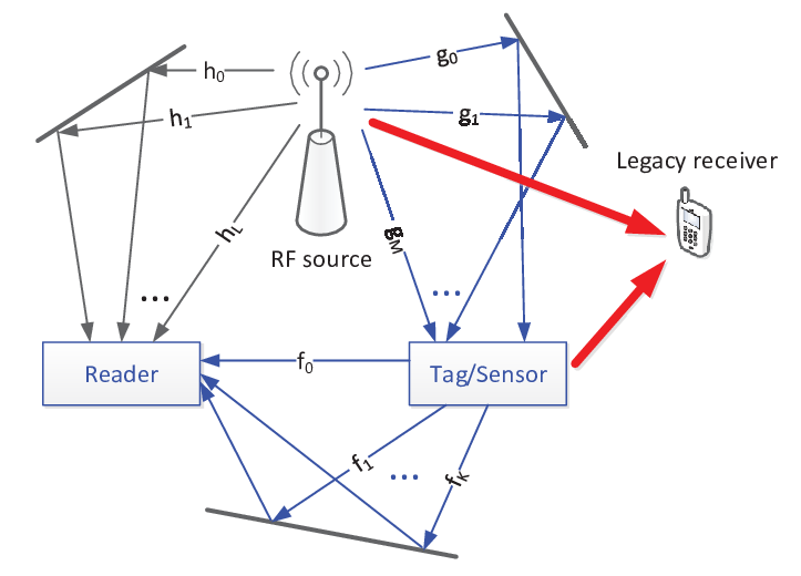
A typical ambient backscatter communication system includes three components: a radio frequency (RF) source, a tag (or a sensor), and a reader, as shown in Fig. 1. The communication process between the tag and the reader mainly contains two steps: first, the tag harvests energy from the signals of the RF source; second, the tag modulates its binary information onto the received RF signals and then backscatters them to the reader.

Almost all existing studies [1, 2, 3, 4, 5, 6, 7] about ambient backscatter communication are based on the assumption of flat-fading channels. However, the frequency-selective channels often exist in many practical scenarios. For ambient backscatter communication systems, frequency-selective channels may result in multiple copies of backscattered signals at the reader, together with multiple source signals. Accordingly, it is one challenging problem for the reader to decode and recover the tag signals.

In this paper, we investigate the ambient backscatter communication systems over frequency-selective channels and propose a transceiver design to cope with the signal detection challenge at the reader. Our design smartly utilizes the cyclic prefix (CP) of orthogonal frequency-division multiplexing (OFDM) source symbols, which can facilitate signal detection at the reader via cancelling the signal interference. Moreover, different from the transceiver design in [4], our design leads to no interference to the legacy receivers. A chi-square based detector is then proposed and the corresponding optimal detection threshold is derived. Simulation results show that our transceiver design for the frequency-selective channels is efficient and achieves low bit error rate (BER) due to interference cancellation.

Refer to caption — Fig. 1: System model.

The rest of this paper is organized as follows: Section II formulates the model of the ambient backscatter communication system over frequency-selective channels. Section III proposes the transceiver design and Section IV derives the chi-square based detector together with the optimal detection threshold. Section V provides the simulation results and finally Section VI summarizes this paper.

II System Model

Consider an ambient backscatter communication system over frequency-selective channels in Fig. 1. The multi-path channels between the RF source and reader, the RF source and tag, the reader and tag are denoted by $h_{l}\,\,(l=0,1,\cdots,L)$ , $g_{m}\,\,(m=0,1,\cdots,M)$ , $f_{k}\,\,(k=0,1,\cdots,K)$ , respectively. Both the reader and the legacy receiver receive signals from the RF source and the tag over frequency-selective channels.

Suppose the signal transmitted by the RF source is $s(n)$ with the zero-mean and the variance of $P_{s}$ and $s(n)\sim\mathcal{CN}(0,P_{s})$ . Due to the multi-path channels $g(m)\,\,(m=0,1,\cdots,M)$ , the signal arriving at the tag antenna can be given as

\displaystyle x(n)=\sum_{m=0}^{M}g_{m}s(n-m).

(1)

The tag next modulates its own binary signal $B(n)$ onto the received signal $x(n)$ to communicate with the reader via backscattering $x(n)$ or not. Specifically, the tag changes its antenna impedance to reflect $x(n)$ to the reader so as to indicate $B(n)=1$ ; and when indicating $B(n)=0$ , the tag switches the impedance to a certain value so that no signal can be reflected. Assume that $B(n)=0$ and $B(n)=1$ are equiprobable.

Finally, the received signal at the reader can be expressed as

\displaystyle y(n)=\sum_{l=0}^{L}h_{l}s(n-l)+\eta\sum_{k=0}^{K}f_{k}B(n-k)x(n-k)+w(n),

(2)

where $\eta$ represents the complex attenuation inside the tag, $w(n)$ denotes the additive white Gaussian noise (AWGN) and we assume $w(n)\sim\mathcal{CN}(0,N_{w})$ .

Remark 1

The reader aims to recover the tag signal $B(n)$ from the received signal $y(n)$ . Nevertheless, since the binary signal $B(n)$ hides in the received signal $y(n)$ , it is inefficient to utilize the methods in traditional point-to-point and relay communication systems to realize the recovery of $B(n)$ . In addition, the frequency-selective channels worsen this dilemma due to multiple copies of the source signals that appear in the received signals $y(n)$ . Consequently, a transceiver design together with a signal detector are required to achieve accurate recovery of $B(n)$ , which will be introduced in our later Section III and Section IV, respectively.

III Interference-free Transceiver Design

In this section, we describe an interference-free transceiver design, whose implementation mainly consists of three crucial aspects: the tag signal design, the signal interference cancelling method, and the discrete Fourier transformation (DFT) operation.

III-A Tag Signal Design

With the assumption that the RF source emits OFDM symbols, the structures of the RF source signal $s(n)$ , the tag signal $B(n)$ , and the received signal $x(n)$ at the tag, are presented in Fig. 2.¹¹ 1 Since the OFDM technique is ubiquitous in current wireless systems such as LTE and WiFi, it is reasonable to consider the RF source emitting OFDM symbols. We set $C$ and $N$ as the lengths of the CP and the effective part of the OFDM symbol, respectively. The parameter $Q$ is defined as $Q={\rm max}\{L,M,K\}$ .

Obviously, both $s(n)$ and $x(n)$ have repeating sequences, even if the signal $x(n)$ experiences the multi-path channels $g(m)\,\,(m=0,1,\cdots,M)$ . Besides, we divide one OFDM symbol period into four phases for the designed tag signal $B(n)$ . In Phase 1, Phase 3, and Phase 4, no received signal $x(n)$ will be reflected, i.e., $B(n)=0$ . In this case, the signals arriving at the reader directly come from the RF source. However, in Phase 2, the tag modulates its binary data onto the signal $x(n)$ from $n=Q$ to $n=C-K-1$ while no signal is backscattered to the reader in the rest of the Phase 2. By exploiting the signals arriving at the reader in Phase 2 and Phase 4, we can cancel the signal interference, which will be presented in the next subsection.

Remark 2

It can be checked from Fig. 2 that the signal structure of $B(n)$ merely effects the samples in the CP of the OFDM symbol. Since the CP will be removed at the legacy receiver, this transceiver design at the tag will lead to no interference to the legacy receivers.

III-B Signal Interference Cancelling Method

Denote the received signals at the reader in Phase 2 and Phase 4 as $y_{1}(n)\,\,\,(n=Q,\cdots,C-1)$ and $y_{2}(n)\,\,\,(n=N+Q,\cdots,N+C-1)$ , respectively. We can obtain

	$\displaystyle y_{1}(n)=$	$\displaystyle\sum_{l=0}^{L}h_{l}s(n-l)+\eta\sum_{k=0}^{K}f_{k}B(n-k)x(n-k)+w_{1}(n),$		(3)
	$\displaystyle y_{2}(n)=$	$\displaystyle\sum_{l=0}^{L}h_{l}s(n-l)+w_{2}(n),$		(4)

where $w_{1}(n)$ and $w_{2}(n)$ are both AWGN. Assume that $w_{1}(n)\sim\mathcal{CN}(0,N_{w})$ and $w_{2}(n)\sim\mathcal{CN}(0,N_{w})$ .

Apparently, the term $\sum_{l=0}^{L}h_{l}s(n-l)$ in (3) and (4) carries no tag binary information and thus is the interference for the tag signal recovery at the reader, which should be cancelled so as to enhance detection accuracy.

Signal interference cancelling is implemented via subtracting $y_{2}(n)$ from $y_{1}(n)$ , thus the received signals can be written as

$\displaystyle z(n)=$	$\displaystyle y_{1}(n+Q)-y_{2}(n+N+Q)$
$\displaystyle=$	$\displaystyle\eta\sum_{k=0}^{K}f_{k}B(n-k)x(n-k)+w_{1}(n)-w_{2}(n),$
$\displaystyle=$	$\displaystyle\eta\sum_{k=0}^{K}f_{k}B(n-k)x(n-k)+w_{e}(n),$	(5)

where $n=0,1,\cdots,C-Q-1$ and $w_{e}(n)\sim\mathcal{CN}(0,2N_{w})$ .

Assuming $T=C-Q-1$ and $R=C-Q-K-1$ , we rewrite (5) in matrix as

	$\displaystyle\begin{pmatrix}z(0)\\ z(1)\\ \vdots\\ z(n)\\ \vdots\\ z(T)\end{pmatrix}=\eta\begin{pmatrix}f_{0}&0&\cdots&0&\cdots&0&0\\ f_{1}&f_{0}&\cdots&0&\cdots&0&0\\ \vdots&\vdots&\cdots&\vdots&\cdots&\vdots&\vdots\\ f_{K}&f_{K-1}&\cdots&f_{0}&\cdots&0&0\\ \vdots&\vdots&\cdots&\vdots&\cdots&\vdots&\vdots\\ 0&0&\cdots&0&\cdots&f_{0}&0\\ 0&0&\cdots&0&\cdots&f_{1}&f_{0}\\ \vdots&\vdots&\cdots&\vdots&\cdots&\vdots&\vdots\\ 0&0&\cdots&0&\cdots&f_{K-1}&f_{K-2}\\ 0&0&\cdots&0&\cdots&f_{K}&f_{K-1}\\ 0&0&\cdots&0&\cdots&0&f_{K}\end{pmatrix}$
	$\displaystyle\begin{pmatrix}B(0)x(0)\\ B(1)x(1)\\ \vdots\\ B(n)x(n)\\ \vdots\\ B(R)x(R)\end{pmatrix}+\begin{pmatrix}w_{e}(0)\\ w_{e}(1)\\ \vdots\\ w_{e}(n)\\ \vdots\\ w_{e}(T)\end{pmatrix}.$		(6)

III-C DFT Operation

After signal interference cancelling at the reader, let us construct the signal vector z as

	$\displaystyle\textbf{z}=$	$\displaystyle[z(0)+z(R+1),\cdots,z(T-R-1)+z(T),$
		$\displaystyle\qquad\qquad\,\,\,\,\,z(T-R),\cdots,z(R-1),z(R)]^{\rm T}.$		(7)

Define

$\displaystyle\textbf{b}=$	$\displaystyle[B(0),B(1),\cdots,B(n),\cdots,B(R)],$	(8)
$\displaystyle\textbf{x}=$	$\displaystyle[x(0),x(1),\cdots,x(n),\cdots,x(R)]^{\rm T},$	(9)
$\displaystyle\textbf{w}=$	$\displaystyle[w_{e}(0)+w_{e}(R+1),\cdots,w_{e}(T-R-1)+w_{e}(T),$
	$\displaystyle\qquad\qquad\;\,w_{e}(T-R),\cdots,w_{e}(R-1),w_{e}(R)]^{\rm T}.$	(10)

Denote F as the $(R+1)\times(R+1)$ DFT matrix with the $(p,q)$ th element $\textbf{F}_{pq}=\exp(-j2\pi pq/(R+1))$ . Let us consider a Toeplitz matrix T, which possesses the first row of $\textbf{t}_{\textbf{r}}=[f_{0},0,\cdots,0,f_{K},f_{K-1},\cdots,f_{k},\cdots,f_{1}]$ and the first column of $\textbf{t}_{\textbf{c}}=[f_{0},f_{1},\cdots,f_{k},\cdots,f_{K},0,\cdots,0]^{\rm T}$ .

Consequently, we reconstruct the signal vector z based on DFT as, i.e., DFT outputs $\tilde{\textbf{z}}$

$\displaystyle\tilde{\textbf{z}}=$	Fz
$\displaystyle=$	$\displaystyle\,\eta\textbf{F}\textbf{T}\cdot{\rm diag}[\textbf{b}]\cdot\textbf{x}+\textbf{F}\textbf{w}$
$\displaystyle=$	$\displaystyle\,\eta\cdot{\rm diag}\left[\tilde{\textbf{f}}^{\rm T}\right]\cdot{\rm diag}[\textbf{b}]\cdot\tilde{\textbf{x}}+\tilde{\textbf{w}},$	(11)

where

$\displaystyle\tilde{\textbf{z}}=\,$	$\displaystyle[\tilde{z}(0),\tilde{z}(1),\cdots,\tilde{z}(n),\cdots,\tilde{z}(R)]^{\rm T}=\textbf{F}\textbf{z},$	(12)
$\displaystyle\tilde{\textbf{x}}=\,$	$\displaystyle[\tilde{x}(0),\tilde{x}(1),\cdots,\tilde{x}(n),\cdots,\tilde{x}(R)]^{\rm T}=\textbf{F}\textbf{x},$	(13)
$\displaystyle\tilde{\textbf{w}}=\,$	$\displaystyle[\tilde{w}_{e}(0),\tilde{w}_{e}(1),\cdots,\tilde{w}_{e}(n),\cdots,\tilde{w}_{e}(R)]^{\rm T}=\textbf{F}\textbf{w},$	(14)
$\displaystyle\tilde{\textbf{f}}=\,$	$\displaystyle[\tilde{f}_{0},\tilde{f}_{1},\cdots,\tilde{f}_{n},\cdots,\tilde{f}_{R}]^{\rm T}=\textbf{F}\textbf{t}_{\textbf{r}}^{\rm T}.$	(15)

According to the central limit theorem (CLT) [8], we assume $\tilde{x}(n)\sim\mathcal{CN}(0,P_{x})$ , $\tilde{w}_{e}(n)\sim\mathcal{CN}(0,P_{w})$ and $\tilde{f}_{n}\sim\mathcal{CN}(0,P_{f})$ , where

$\displaystyle P_{x}=$	$\displaystyle(R+1)P_{s}\sum_{m=0}^{M}\|g_{m}\|^{2},$	(16)
$\displaystyle P_{w}=$	$\displaystyle 2(T+1)N_{w},$	(17)
$\displaystyle P_{f}=$	$\displaystyle\sum_{k=0}^{K}\|f_{k}\|^{2}.$	(18)

IV Chi-square Based Signal Detection at the Reader

In this section, the chi-square based detector together with the optimal detection threshold are derived via the maximum likelihood (ML) principle. The corresponding BER expression is also obtained to evaluate the detection performance.

IV-A Chi-square Based Detector

Due to the lower data-rate of the tag signal $B(n)$ than that of the signal $\tilde{z}(n)$ , we suppose the signal $B(n)$ remains equivalent within $W$ samples of $\tilde{z}(n)$ . Let us construct the test statistic for detecting $B(n)$ as

\displaystyle\Gamma_{t}=\frac{1}{P_{w}}\sum_{n=(t-1)W+1}^{tW}\left|\tilde{z}(n)\right|^{2},

(19)

where $t=1,2,\cdots,T$ , and $\tilde{z}(n)$ is expanded as

\displaystyle\tilde{z}(n)=\left\{\begin{aligned} &\tilde{w}_{e}(n),&{\rm if}\,\,\,B(n)=0,\\ &\eta\tilde{f}_{n}\tilde{x}(n)+\tilde{w}_{e}(n),&{\rm if}\,\,\,B(n)=1.\\ \end{aligned}\right.

(20)

It can be readily checked that

\displaystyle\Gamma_{t}=\left\{\begin{aligned} &M_{t},&{\rm if}\,\,\,B(n)=0,\\ &J_{t}+M_{t}+V_{t},&{\rm if}\,\,\,B(n)=1,\\ \end{aligned}\right.

(21)

where

$\displaystyle M_{t}=$	$\displaystyle\frac{1}{P_{w}}\sum_{n=(t-1)W+1}^{tW}\left\|\tilde{w}_{e}(n)\right\|^{2},$	(22)
$\displaystyle J_{t}=$	$\displaystyle\frac{1}{P_{w}}\sum_{n=(t-1)W+1}^{tW}(\|\eta\|^{2}\left\|\tilde{f}_{n}\right\|^{2}\left\|\tilde{x}(n)\right\|^{2}),$	(23)
$\displaystyle V_{t}=$	$\displaystyle\frac{1}{P_{w}}\sum_{n=(t-1)W+1}^{tW}(2\mathcal{R}\{\eta\tilde{f}_{n}\tilde{x}(n){\tilde{w}^{*}_{e}(n)}\}).$	(24)

Let $\mathcal{H}_{1}$ and $\mathcal{H}_{0}$ represent $B(n)=1$ and $B(n)=0$ , respectively. Apparently, under $\mathcal{H}_{1}$ , the test statistic $\Gamma_{t}$ follows the noncentral chi-square distribution with $W$ degrees of freedom and noncentrality parameter $\lambda=W\gamma$ [9], i.e., $\Gamma_{t}\sim\chi^{2}_{W}(\lambda)$ , where $\gamma$ is the detection signal-to-noise ratio (SNR) that can be calculated as

\displaystyle\gamma=\frac{|\eta|^{2}P_{x}P_{f}}{P_{w}}=\frac{(R+1)|\eta|^{2}P_{s}\sum_{m=0}^{M}|g_{m}|^{2}\sum_{k=0}^{K}|f_{k}|^{2}}{2(T+1)N_{w}}.

(25)

While under $\mathcal{H}_{0}$ , $\Gamma_{t}$ follows the chi-square distribution with $W$ degrees of freedom, which is denoted as $\Gamma_{t}\sim\chi^{2}_{W}(0)$ .

Therefore, the probability density function (PDF) of $\Gamma_{t}$ under $\mathcal{H}_{0}$ is obtained as

\displaystyle{\rm Pr}(\Gamma_{t}|\mathcal{H}_{0})=f_{0}(\Gamma_{t},W),

(26)

where

\displaystyle f_{0}(x,n)=\left\{\begin{aligned} &\frac{1}{2^{\frac{n}{2}}\Gamma(n/2)}{\rm e}^{-\frac{x}{2}}x^{\frac{n}{2}-1},&{\rm if}\,\,\,x>0,\\ &0,&{\rm if}\,\,\,x\leq 0,\\ \end{aligned}\right.

(27)

and $\Gamma(x)=\int_{0}^{\infty}{\rm e}^{-t}t^{x-1}{\rm d}t$ as the Gamma function [10].

Similarly, under $\mathcal{H}_{1}$ , the PDF of $\Gamma_{t}$ is

\displaystyle{\rm Pr}(\Gamma_{t}|\mathcal{H}_{1})=f_{1}(\Gamma_{t},W,\lambda),

(28)

where

\displaystyle f_{1}(x,n,\lambda)=\left\{\begin{aligned} &\frac{1}{2}\left(\frac{x}{\lambda}\right)^{\frac{n-2}{4}}{\rm e}^{-\frac{x+\lambda}{2}}I_{\frac{n}{2}-1}\left(\sqrt{\lambda x}\right),&{\rm if}\,\,\,x>0,\\ &0,&{\rm if}\,\,\,x\leq 0,\\ \end{aligned}\right.

(29)

and $I_{r}(u)$ is the $r$ -order modified Bessel function of the first kind [10]

\displaystyle I_{r}(u)=\frac{\left(\frac{1}{2}u\right)^{r}}{\sqrt{\pi}\Gamma(r+\frac{1}{2})}\int_{0}^{\pi}{\rm e}^{u\cos\theta}\sin^{2r}{\theta}{\rm d}\theta.

(30)

Consequently, the chi-square based detector can be made through the ML principle as

\displaystyle\hat{B}(n)=\mathop{\arg\max}\limits_{B(n)\in\{0,1\}}{\rm Pr}(\Gamma_{t}|B(n)),

(31)

where ${\rm Pr}(\Gamma_{t}|B(n))$ is the probability density function (PDF) of $\Gamma_{t}$ given $B(n)$ . We can also reformulate the ML detection rule (31) as

\displaystyle\hat{B}(n)=\left\{\begin{aligned} &0,&{\rm if}\,\,\,{\rm Pr}(\Gamma_{t}|\mathcal{H}_{0})>{\rm Pr}(\Gamma_{t}|\mathcal{H}_{1}),\\ &1,&{\rm if}\,\,\,{\rm Pr}(\Gamma_{t}|\mathcal{H}_{0})<{\rm Pr}(\Gamma_{t}|\mathcal{H}_{1}).\\ \end{aligned}\right.

(32)

One example of the PDFs of $\Gamma_{t}$ under two conditions $\mathcal{H}_{0}$ and $\mathcal{H}_{1}$ is presented in Fig. 3.

IV-B Optimal Detection Threshold

The optimal detection threshold $T_{h}$ of this ML detector can be derived by setting that the PDF under $\mathcal{H}_{0}$ equals to that under $\mathcal{H}_{1}$

\displaystyle{\rm Pr}(\Gamma_{t}|\mathcal{H}_{0})={\rm Pr}(\Gamma_{t}|\mathcal{H}_{1})\big|_{\Gamma_{t}=T_{h}}.

(33)

Define

\displaystyle I=\int_{0}^{\pi}{\rm e}^{\sqrt{W\gamma T_{h}}}{\rm e}^{\cos\theta}\sin^{W-2}{\theta}{\rm d}\theta.

(34)

Substituting (27) and (29) into (33) will produce

\displaystyle\frac{T_{h}^{\frac{W-2}{4}}{\rm e}^{-\frac{T_{h}+W\gamma}{2}}\left(W\gamma T_{h}\right)^{\frac{W-2}{4}}}{2^{\frac{W}{2}}\sqrt{\pi}\left(W\gamma\right)^{\frac{W-2}{4}}\Gamma\left(\frac{W}{2}-\frac{1}{2}\right)}I=\frac{{\rm e}^{-\frac{T_{h}}{2}}T_{h}^{\frac{W-2}{2}}}{2^{\frac{W}{2}}\Gamma{\left(\frac{W}{2}\right)}},

(35)

which can be further simplified as

\displaystyle\frac{{\rm e}^{-\frac{W\gamma}{2}}I}{\sqrt{\pi}\Gamma{\left(\frac{W}{2}-\frac{1}{2}\right)}}=\frac{1}{\Gamma\left(\frac{W}{2}\right)}.

(36)

After exerting some mathematical manipulations in (36), one obtains

\displaystyle T_{h}=\left(\ln{\frac{\sqrt{\pi}\Gamma{\left(\frac{W}{2}-\frac{1}{2}\right)}}{{\rm e}^{-\frac{W\gamma}{2}}\Gamma\left(\frac{W}{2}\right)\int_{0}^{\pi}{\rm e}^{\cos\theta}\sin^{W-2}{\theta}{\rm d}\theta}}\right)^{2}\bigg/(W\gamma).

(37)

Therefore, the detection rule can be summarized as

\displaystyle\hat{B}(n)=\left\{\begin{matrix}0,&{\rm if}\,\,\,\Gamma_{t}<T_{h},\\ 1,&{\rm if}\,\,\,\Gamma_{t}>T_{h}.\end{matrix}\right.

(38)

IV-C BER Performance

Define $p_{0}={\rm Pr}(\hat{B}(n)=1|B(n)=0)$ and $p_{1}={\rm Pr}(\hat{B}(n)=0|B(n)=1)$ as the probability of false alarm and the probability of missing detection, separately.

The BER of the chi-square based detector is given by

	$\displaystyle P_{e}=$	$\displaystyle{\rm Pr}(B(n)=0)p_{0}+{\rm Pr}(B(n)=1)p_{1}$
	$\displaystyle=$	$\displaystyle\frac{1}{2}\left(p_{0}+p_{1}\right).$		(39)

By utilizing the approximations in [9], we can further derive the BER $P_{e}$ as

\displaystyle P_{e}\approx\frac{1}{2}Q\left(\frac{T_{h}-W}{\sqrt{2W}}\right)+\frac{1}{2}Q\left(\frac{W(1+\gamma)-T_{h}}{\sqrt{2W(1+2\gamma)}}\right),

(40)

where $Q(\cdot)$ denotes the Gaussian Q-function [10]

\displaystyle Q(x)=\frac{1}{\sqrt{2\pi}}\int_{x}^{\infty}{\rm e}^{-\frac{t^{2}}{2}}{\rm d}t.

(41)

V Simulation Results

In this section, numerical results are provided to assess the performance of proposed chi-square based detector. All the channels follow Gaussian distributions with the zero-mean and unit-variance. The number of channel taps $L+1$ , $M+1$ and $K+1$ are assumed to be $6$ in following simulations. We set the attenuation $|\eta|$ , the noise power $N_{w}$ and the length of CP $C$ as $0.5$ , $1$ and $256$ , separately. We also exert $10^{7}$ Monte Carlo trials for every experiment to examine BER performance of the chi-square based detector.

Fig. 4 plots the BER curves versus SNR for the chi-square based detector with the optimal detection threshold. We set the number of averaging samples $W$ as $3$ and $12$ , respectively. As seen, the BER performance could be enhanced with enlarging SNR or $W$ .

Fig. 5 depicts the BER curves versus the number of averaging samples $W$ with different SNR for our detector. We choose SNR as 13 dB and 16 dB, separately. It is found that the BER performance is improved with increasing $W$ . Besides, due to the exploitation of the approximation (40) for analytical BER, there is a small gap between the simulation and analytical results in Fig. 5.

VI Conclusion

This paper focused on the data transmission of the ambient backscatter communication systems over frequency-selective channels. A novel interference-free transceiver design, which exploits the CP structure of OFDM symbols to cancel the signal interference, was proposed to facilitate interference cancellation and signal detection in such scenario. Moreover, this transceiver design led to no interference to the legacy receivers since the CP will be removed at the legacy receiver. Furthermore, a chi-square based detector was derived, as well as the optimal detection threshold. Finally, the BER performance of the chi-square based detector was evaluated via Monte Carlo simulations. It was shown that the proposed transceiver design is efficient and the chi-square based detector demonstrates satisfying BER performance.

References

[1] V. Liu, A. Parks, V. Talla, S. Gollakota, D. Wetherall, and J. R. Smith, “Ambient backscatter: wireless communication out of thin air,” in Proc. ACM SIGCOMM, Hong Kong, China, 2013, pp. 1-13.
[2] G. Wang, F. Gao, R. Fan, and C. Tellambura, “Ambient backscatter communication systems: detection and performance analysis,” IEEE Trans. Commun., vol. 64, no. 11, pp. 1-10, Aug. 2016.
[3] J. Qian, F. Gao, G. Wang, S. Jin, and H. Zhu, “Noncoherent detections for ambient backscatter system,” IEEE Trans. Wireless Commun., vol. 16, no. 3, pp. 1412-1422, Mar. 2017.
[4] G. Yang, Y. C. Liang, R. Zhang, and Y. Pei, “Modulation in the air: backscatter communication over ambient OFDM carrier,” IEEE Trans. Commun., vol. 66, no. 3, pp. 1219-1233, Mar. 2018.
[5] S. Ma, G. Wang, R. Fan, and C. Tellambura, “Blind channel estimation for ambient backscatter communication systems,” IEEE Commun. Lett., vol. 22, no. 6, pp. 1296-1299, Jun. 2018.
[6] Z. Ma, T. Zeng, G. Wang, and F. Gao, “Signal detection for ambient backscatter system with multiple receiving antennas,” in Proc. IEEE 14th Can. Workshop Inf. Theory (CWIT), St. John¡¯s, NF, Canada, Jul. 2015, pp. 1-4.
[7] D. Li, W. Peng, and Y. Liang, “Hybrid ambient backscatter communication systems with harvest-then-transmit protocols,” IEEE Access, vol. 6, pp. 45288-45298, 2018.
[8] A. Papoulis and S. U. Pillai, Probability, Random Variables and Stochastic Processes. 4th ed. New York, NY, USA: McGraw-Hill, 2002, ch. 7, pp. 278-279.
[9] D. Horgan and C. C. Murphy, ”On the convergence of the chi square and noncentral chi square distributions to the normal distribution,” IEEE Commun. Lett., vol. 17, no. 12, pp. 2233-2236, Dec. 2013.
[10] I. M. Ryzhik, A. Jeffrey, and D. Zwillinger, Table of Integrals, Series and Products. San Diego, CA, USA: Academic, 2007.