Storage capacity in symmetric binary perceptrons

Benjamin Aubin Affiliation: Institut de physique théorique, Université Paris Saclay, CNRS, CEA Saclay, F-91191 Gif-sur-Yvette, France Will Perkins Affiliation: Department of Mathematics, Statistics and Computer Science, University of Illinois, Chicago, USA Lenka Zdeborová Affiliation: Institut de physique théorique, Université Paris Saclay, CNRS, CEA Saclay, F-91191 Gif-sur-Yvette, France

August 11, 2026

Abstract

We study the problem of determining the capacity of the binary perceptron for two variants of the problem where the corresponding constraint is symmetric. We call these variants the rectangle-binary-perceptron (RPB) and the $u-$ function-binary-perceptron (UBP). We show that, unlike for the usual step-function-binary-perceptron, the critical capacity in these symmetric cases is given by the annealed computation in a large region of parameter space (for all rectangular constraints and for narrow enough $u-$ function constraints, $K<K^{*}$ ). We prove this fact (under two natural assumptions) using the first and second moment methods. We further use the second moment method to conjecture that solutions of the symmetric binary perceptrons are organized in a so-called frozen-1RSB structure, without using the replica method. We then use the replica method to estimate the capacity threshold for the UBP case when the $u-$ function is wide $K>K^{*}$ . We conclude that full-step-replica-symmetry breaking would have to be evaluated in order to obtain the exact capacity in this case.

I Introduction

In this paper we revisit the problem of computing the capacity of the binary perceptron 1; 2 for storing random patterns. This problem lies at the core of early statistical physics studies of neural networks and their learning and generalization properties, for reviews see e.g. watkin1993statistical; seung1992statistical; engel2001statistical; NishimoriBook01. While the perceptron problem is motivated by studies of simple artificial neural networks as discussed in detail in the above literature, in this paper we view it as a random constraint satisfaction problem (CSP) where the vector of binary weights $\textbf{w}\in\{\pm 1\}^{N}$ (a solution) must satisfy $M$ step constraints of the type

\sum_{i=1}^{N}X_{\mu i}w_{i}\geq K\,,

(1)

where $\mu=1,\dots,M$ , $K\in\mathbbm{R}$ is the threshold, the random variables $X_{\mu i}$ are $iid$ Gaussian variables with zero mean and variance $1/N$ , and the rows of the matrix ${\mathbb{X}}\in\mathbb{R}^{M\times N}$ are called patterns. We define an indicator function associated to the perceptron with a step constraint as $\varphi^{s}(z)=\mathbbm{1}_{\displaystyle z\geq K}$ .

We say that a given vector w is a solution of the perceptron instance if all $M$ constraints given by eq. (1) are satisfied. The storage capacity is then defined similarly to the satisfiability threshold in random constraint satisfaction problems: we denote the constraint density as $\alpha\equiv M/N$ and define the storage capacity $\alpha_{c}(K)$ as the infimum of densities $\alpha$ such that in the limit $N\to\infty$ , with high probability (over the choice of the matrix ${\mathbb{X}}$ ) there are no solutions. It is natural to conjecture that the converse also holds, i.e. the storage capacity $\alpha_{c}(K)$ equals the supremum of $\alpha$ such that in the limit $N\to\infty$ solutions exist with high probability. In this case we would say the storage capacity is a sharp threshold.

Gardner and Derrida in their paper 1 assume the storage capacity $\alpha_{c}(K)$ is a sharp threshold and they apply the replica calculation to compute it, but reach a result inconsistent with a simple upper bound obtained by the first moment method. Mézard and Krauth 2 found a way to obtain a consistent prediction from the replica calculation and concluded that the storage capacity $\alpha^{s}_{c}(K)$ for the step binary perceptron (SBP), i.e. associated to the constraint $\varphi^{s}$ , is given by the largest $\alpha$ for which the following quantity, the entropy in physics, is positive:

\phi_{\rm RS}^{s}(\alpha,K)=\textrm{extr}_{q_{0},\hat{q}_{0}}\left\{\frac{1}{2}\left(q_{0}-1\right)\hat{q}_{0}+\int Dt\log\left[2\cosh\left(t\sqrt{\hat{q}_{0}}\right)\right]+\alpha\int Dt\log\left[\int^{\infty}_{\frac{K-t\sqrt{q_{0}}}{\sqrt{1-q_{0}}}}Du\right]\right\}\,,

(2)

where $Dt=\frac{e^{-t^{2}/2}}{\sqrt{2\pi}}dt$ is a normal Gaussian measure, and ” $\rm extr$ ” means that the expression is evaluated where the derivatives on the curl-bracket, with respect to $q_{0}\geq 0$ and $\hat{q}_{0}\geq 0$ , are zero.

Several decades of subsequent research in the statistical physics of disordered systems are consistent with the conjectured Mézard-Krauth formula for the storage capacity of the binary perceptron. Despite the simplicity of the above conjecture and decades of impressive progress in the mathematics of spin glasses and related problems, (see e.g. talagrand2006parisi; talagrand2003spin; 8; achlioptas2011solution; panchenko2014parisi; ding2015proof and many others), the storage capacity of the binary perceptron remains an open mathematical problem. In fact, even the very existence of a sharp threshold, i.e. the fact that in the limit $N\to\infty$ the probability that patterns can be stored drops sharply from one to zero at the capacity, is an open problem. Up to very recently only widely non-matching upper bounds and lower bounds for the storage capacity of the binary perceptron were available kim1998covering; stojnic2013discrete. As the present work was being finalized Ding and Sun ding2018capacity proved in a remarkable paper a lower bound on the capacity that matches the Krauth and Mezard conjecture (note that much like Theorem 4 below, the main theorem in ding2018capacity depends on a numerical hypothesis). A matching upper bound remains an open challenge in mathematical physics and probability theory.

In this paper we introduce two simple symmetric variants of the binary perceptron problem. Let $z_{\mu}(\textbf{w})=\sum_{i=1}^{N}X_{\mu i}w_{i}$ . For a threshold $K\in\mathbbm{R}^{+}$ , we consider two different types of symmetric constraints:

•

The rectangle binary perceptron (RBP) requires $|z_{\mu}|\leq K,\forall\mu=1,\dots,M$ . Its associated indicator function is $\varphi^{r}(z)=\mathbbm{1}_{\displaystyle|z|\leq K}$ .
•

The $u$ -function binary perceptron (UBP) requires $|z_{\mu}|\geq K,\forall\mu=1,\dots,M$ . Its associated indicator function is $\varphi^{u}(z)=\mathbbm{1}_{\displaystyle|z|\geq K}$ .

These constraints are symmetric in the sense that if w is a solution then $-\textbf{w}$ is a solution as well. Our motivation behind these symmetric variants of the perceptron is that this symmetry simplifies greatly the mathematical treatment of the problem, while keeping the relevant physical properties intact. Thus, results that remain open questions for the canonical perceptron can be established rigorously for these symmetric versions. Symmetric perceptron models are also directly related to the problem of determining the discrepancy of a random matrix or set system BansalSpencer19, a problem of interest in combinatorics.

The main result of the present paper, presented in section II, is a proof, subject to a numerical hypothesis, of a formula for the storage capacity, defined in the same way as for the step-function binary perceptron above. In particular, we show that in these symmetric variants the first moment upper bound (corresponding to the annealed capacity in physics) on the storage capacity is tight (except for $K>K^{*}\simeq 0.817$ for the UBP case). We prove this statement using the second moment method. We note that the existing physics literature on perceptron-like problem contains other cases of models where the first moment upper bound on the storage capacity was observed to be tight, in particular the parity machine opper1995statistical, and the reversed-wedge binary perceptron bex1995storage; hosaka2002statistical. Those works, however, rely on the comparison of the first moment bound on the capacity with the result of the replica method, rather than providing a rigorous justification.

To formally state our main result, let $Z\sim\mathcal{N}(0,1)$ , and for $K\in\mathbbm{R}^{+}$ let $p_{r,K}=\mathbb{P}[|Z|\leq K]$ and $p_{u,K}=\mathbb{P}[|Z|\geq K]$ .

•

The storage capacity for the rectangle binary perceptron is:

$\alpha_{c}^{r}(K)=\frac{-\log(2)}{\log(p_{r,K})}\hskip 14.22636pt\forall K\in\mathbb{R}^{+}\,.$ (3)
•

The storage capacity for the $u-$ function binary perceptron is:

$\alpha_{c}^{u}(K)=\frac{-\log(2)}{\log(p_{u,K})}\hskip 14.22636pt{\rm for}\hskip 5.69046pt0<K<K^{*}\simeq 0.817\,.$ (4)

The constant $K^{*}\simeq 0.817$ stems from the properties of the second moment entropy eq. (10). In the physics terms it is defined as the point of intersection between the annealed capacity $\alpha_{a}^{u}(K)$ and the local stability of the RS solution $\alpha_{\rm AT}^{u}(K)$ eq. (17). That is, $K^{*}$ is the solution of the following equation:

\pi p_{u,K}^{2}e^{K^{2}}\log(p_{u,K})=-2\log(2)K^{2}\,.

(5)

The two symmetric variants of the perceptron problem considered here share many of the intriguing geometric properties of the original step-function binary perceptron problem. Most significant is the conjectured frozen-1RSB 2 nature of the space of solutions that splits into well separated clusters of vanishing entropy at any $\alpha>0$ . Remarkably, this frozen-1RSB property can be deduced from the form of the second moment entropy as we explain in section III. Our justification of the frozen-1RSB property does not rely on the replica method and is hence of independent interest.

For the UBP and $K>K^{*}$ , the second-moment proof technique fails, and this failure marks tightly the onset of the replica symmetry breaking region. In that region, we evaluate the one-step replica symmetry breaking (1RSB) approximation for the storage capacity, but conclude that full-step replica symmetry breaking (FRSB) would be needed to obtain the exact result. While the FRSB equations can be written along the lines of 20, they are more involved than the ones for the Sherrington-Kirkpatrick model parisi1979infinite; parisi1980sequence; parisi1980order, and solving them numerically or getting additional insight from them is a challenging task left for future work. We present the replica analysis in section IV. Table 1 contains the summary of our main results along with the predictions for the step-function perceptron.

Binary perceptron	Constraint	Constraint function	Range of $K$	Storage capacity
Step-function	$z\geq K$	$\varphi^{s}(z)=\mathbbm{1}_{\displaystyle z\geq K}$	$\forall K\in{\mathbb{R}}$	RS eq. (2)
Rectangle	$\|z\|\leq K$	$\varphi^{r}(z)=\mathbbm{1}_{\displaystyle\|z\|\leq K}$	$\forall K\in{\mathbb{R}}^{+}$	Annealed eq. (3)
$U$ -function	$\|z\|\geq K$	$\varphi^{u}(z)=\mathbbm{1}_{\displaystyle\|z\|\geq K}$	$0<K<K^{*}=0.817$	Annealed eq. (4)
$U$ -function	$\|z\|\geq K$	$\varphi^{u}(z)=\mathbbm{1}_{\displaystyle\|z\|\geq K}$	$\forall K>K^{*}=0.817$	FRSB?

Table 1: This table summarizes results for storage capacity in binary perceptrons with different types of constraints. The result for canonical step-function is from 2. The results for the rectangle and

u

-function are obtained in this paper.

Finally let us comment on the simpler and more commonly considered case of spherical perceptron where the binary constraint on the vector ${\mathbb{w}}$ is replaced by the spherical constraint ${\mathbb{w}}^{\intercal}{\mathbb{w}}=\sum_{i=1}^{N}w^{2}_{i}=N$ . For $K=0$ the spherical perceptron reduces to the famous problem of intersection of half-spaces with capacity $\alpha_{c}=2$ as solved by Wendell wendel1962problem and Cover cover1965geometrical. For $K>0$ the Gardner-Derrida solution 1 is correct as proven in shcherbina2003rigorous; stojnic2013another. For $K<0$ the situation is more challenging and FRSB is needed to compute the storage capacity; for recent progress in physics see franz2016simplest; 20, while mathematical considerations about this case were presented in stojnic2013negative.

II Proof of correctness of the annealed capacity

To state the main results precisely we introduce some definitions. Let ${\mathbb{X}}({N,M})$ be the random $M\times N$ pattern matrix. Define the partition functions

\displaystyle\mathcal{Z}_{r}({\mathbb{X}})=\displaystyle\sum_{\textbf{w}\in\{\pm 1\}^{N}}\prod_{\mu=1}^{M}\varphi^{r}(\displaystyle z_{\mu}(\textbf{w}))\hskip 8.5359pt\textrm{ and }\hskip 8.5359pt\mathcal{Z}_{u}({\mathbb{X}})=\displaystyle\sum_{\textbf{w}\in\{\pm 1\}^{N}}\prod_{\mu=1}^{M}\varphi^{u}(\displaystyle z_{\mu}(\textbf{w}))\,,

which count respectively the number of solutions for the rectangle and $u-$ function constraints respectively. Let $\mathcal{E}^{r}(N,M)$ and $\mathcal{E}^{u}(N,M)$ be the events that $\mathcal{Z}_{r}({\mathbb{X}})\geq 1$ and $\mathcal{Z}_{u}({\mathbb{X}})\geq 1$ . We formally define the storage capacity.

Defintition 1.

The storage capacity $\alpha_{c}^{r}(K)$ is

\displaystyle\alpha_{c}^{r}(K)

\displaystyle=\inf\{\alpha:\lim_{N\to\infty}\mathbb{P}[\mathcal{E}^{r}(N,\lfloor\alpha N\rfloor)]=0\}\,,

and likewise for $\alpha_{c}^{u}(K)$ .

It is believed that there is a sharp threshold for the existence of solutions.

Conjecture 2.

The storage capacity is a sharp threshold:

\displaystyle\alpha^{r}_{c}(K)

\displaystyle=\sup\{\alpha:\lim_{N\to\infty}\mathbb{P}[\mathcal{E}^{r}(N,\lfloor\alpha N\rfloor)]=1\}\,,

and likewise for $\alpha_{c}^{u}(K)$ .

The corresponding conjecture for the random k-SAT model is the celebrated ‘satisfiability threshold conjecture’ proved for $k$ large by Ding, Sly, and Sun ding2015proof.

Next, couple two standard Gaussians $Z_{1},Z_{\beta}$ by letting $Z$ and $Z^{\prime}$ be independent standard Gaussians and setting $Z_{1}=\sqrt{\beta}Z+\sqrt{1-\beta}Z^{\prime}$ and $Z_{\beta}=\sqrt{\beta}Z-\sqrt{1-\beta}Z^{\prime}$ . Let

\displaystyle\begin{cases}q_{r,K}(\beta)&=\mathbb{P}[|Z_{1}|\leq K\wedge|Z_{\beta}|\leq K]=q_{K}(\beta)\,,\\ q_{u,K}(\beta)&=\mathbb{P}[|Z_{1}|\geq K\wedge|Z_{\beta}|\geq K]=1-2p_{r,K}+q_{K}(\beta)\,,\end{cases}

(6)

with $q_{K}(\beta)$ the probability that two standard Gaussians with correlation $2\beta-1$ are both at most $K$ in absolute value, that is:

\displaystyle q_{K}(\beta)

\displaystyle=\frac{1}{2\pi}\int_{-K}^{K}dy\int_{\frac{-K+(1-2\beta)y}{2\sqrt{\beta(1-\beta)}}}^{\frac{K+(1-2\beta)y}{2\sqrt{\beta(1-\beta)}}}e^{-\frac{x^{2}+y^{2}}{2}}dx\,.

Note that $q_{t,K}(1)=p_{t,K}$ and $q_{t,K}(1/2)=p_{t,K}^{2}$ for $t\in\{r,u\}$ . We now introduce the functions that dictate the effectiveness of the second moment bound. Let

	$\displaystyle F_{r,K,\alpha}(\beta)$	$\displaystyle=H(\beta)+\alpha\log q_{r,K}(\beta)$		(7)
	$\displaystyle\vskip 8.5359ptF_{u,K,\alpha}(\beta)$	$\displaystyle=H(\beta)+\alpha\log q_{u,K}(\beta)$		(8)

where $H(\beta)=-\beta\log\beta-(1-\beta)\log(1-\beta)$ is the Shannon entropy function.

We state a numerical hypothesis in terms of the derivatives of these two functions.

Hypothesis 3.

For all choices of $K>0$ and $\alpha>0$ so that $F^{\prime\prime}_{r,K,\alpha}(1/2)<0$ , there is exactly one $\beta\in(1/2,1)$ so that $F^{\prime}_{r,K,\alpha}(\beta)=0$ . The same holds for $F_{u,K,\alpha}$ .

Our main theorem is a proof, under Hypothesis 3, that the storage capacity is given by the annealed computation.

Theorem 4.

Under the assumption of Hypothesis 3, the following hold.

1.

For all $K>0$ , we have $\alpha_{c}^{r}(K)=-\log(2)/\log(p_{r,K})$ .
2.

For all $K\in(0,K^{*})$ , we have $\alpha_{c}^{u}(K)=-\log(2)/\log(p_{u,K})$ .

Under our definition of $\alpha_{c}^{r}(K)$ and $\alpha_{c}^{u}(K)$ , we must prove two statements to show that $\alpha_{c}^{r}(K)=-\log(2)/\log(p_{r,K})$ (and similarly for $\alpha_{c}^{u}(K)$ ). We use the first moment method to show that for $\alpha>-\log(2)/\log(p_{r,K})$ ,
$\lim_{N\to\infty}\Pr(\mathcal{E}^{r}(N,M))=0$ ; then we use the second moment method to show that for $\alpha<-\log(2)/\log(p_{r,K})$ , $\liminf_{N\to\infty}\Pr(\mathcal{E}^{r}(N,M))>0$ (a result analogous to what Ding and Sun prove for the more challenging step binary perceptron ding2018capacity). Conjecture 2 asserts the stronger statement that for $\alpha<-\log(2)/\log(p_{r,K})$ , $\lim_{N\to\infty}\Pr(\mathcal{E}^{r}(N,M))=1$ .

II.1 First moment upper bound

Proposition 5.

1.

If $\alpha>\alpha_{a}^{r}(K)=\frac{-\log(2)}{\log(p_{r,K})}$ , then whp there is no satisfying assignment to the binary perceptron with the rectangle activation function.
2.

If $\alpha>\alpha_{a}^{u}(K)=\frac{-\log(2)}{\log(p_{u,K})}$ , then whp there is no satisfying assignment to the binary perceptron with the $u$ -function activation function.

Proof.

We give the proof for the rectangle function as the proof for the $u$ -function is identical. Let $\epsilon=\alpha-\alpha_{a}^{r}(K)>0$ . Let ${\mathbb{1}}$ denote the vector of dimension $N$ with all $1$ entries.

	$\displaystyle\mathbb{P}[\mathcal{E}^{r}(N,\alpha N)]$	$\displaystyle\leq\mathbb{E}[\mathcal{Z}_{r}({\mathbb{X}}(N,\alpha N))]=2^{N}\mathbb{E}\left[\prod_{\mu=1}^{\alpha N}\mathbbm{1}_{\left\|z_{\mu}({\mathbb{1}})\right\|\leq K}\right]=2^{N}p_{r,K}^{\alpha N}=\exp(N(\log(2)+\alpha\log(p_{r,K})))$
		$\displaystyle=\exp(N\epsilon\log(p_{r,K}))\to 0\text{ as }N\to\infty\,.$

∎

II.2 Second moment lower bound

Proposition 6.

1.

If $\alpha<\frac{-\log(2)}{\log(p_{r,K})}$ , then

$\liminf_{N\to\infty}\mathbb{P}[\mathcal{E}^{r}(N,\alpha N)]>0.$
2.

If $K<K^{*}$ and $\alpha<\frac{-\log(2)}{\log(p_{u,K})}$ , then

$\liminf_{N\to\infty}\mathbb{P}[\mathcal{E}^{u}(N,\alpha N)]>0.$

To prove Proposition 6 we will apply the second-moment method in a similar fashion to Achlioptas and Moore achlioptas2002asymptotic who determined the satisfiability threshold of random $k$ -SAT to within a factor $2$ by considering not-all-equal satisfying assignments (not-all-equal satisfiability (NAE-SAT) constraints are symmetric in the same way the rectangle and $u$ -function constraints are symmetric). Recall the Paley-Zygmund inequality.

Lemma 7.

Let $X$ be a non-negative random variable. Then

\displaystyle\mathbb{P}[X>0]

\displaystyle\geq\frac{\mathbb{E}[X]^{2}}{\mathbb{E}[X^{2}]}\,.

We will also use the following application of Laplace’s method from Achlioptas and Moore achlioptas2002asymptotic.

Lemma 8.

Let $g(\beta)$ be a real analytic function on $[0,1]$ and let

\displaystyle G(\beta)

\displaystyle=\frac{g(\beta)}{\beta^{\beta}(1-\beta)^{1-\beta}}\,.

If $G(1/2)>G(\beta)$ for all $\beta\neq 1/2$ and $G^{\prime\prime}(1/2)<0$ , then there exists constants $c_{1},c_{2}$ so that for all sufficiently large $N$

\displaystyle c_{1}G(1/2)^{N}\leq\sum_{l=0}^{N}\binom{N}{l}g(l/N)^{N}\leq c_{2}G(1/2)^{N}\,.

II.2.1 Rectangle binary perceptron

We calculate

\displaystyle\mathbb{E}[\mathcal{Z}_{r}({\mathbb{X}})^{2}]

\displaystyle=\sum_{{\mathbb{w_{1}}},{\mathbb{w_{2}}}\in\{\pm 1\}^{N}}\mathbb{P}[{\mathbb{w_{1}}},{\mathbb{w_{2}}}\textrm{ satisfying}]=2^{N}\sum_{{\mathbb{w}}\in\{\pm 1\}^{N}}\mathbb{P}[{\mathbb{1}},{\mathbb{w}}\textrm{ satisfying}]=2^{N}\sum_{l=0}^{N}\binom{N}{l}q_{r,K}(l/N)^{\alpha N}\,,

where we recall $q_{r,K}$ from eq. (6). Define

\displaystyle G_{r,K,\alpha}(\beta)

\displaystyle\equiv\exp(F_{r,K,\alpha}(\beta))=\frac{q_{r,K}(\beta)^{\alpha}}{\beta^{\beta}(1-\beta)^{1-\beta}}\,,

(9)

If we can show that $G_{r,K,\alpha}(1/2)>G_{r,K,\alpha}(\beta)$ for all $\beta\neq 1/2$ and $G_{r,K,\alpha}^{\prime\prime}(1/2)<0$ , then by Lemma 8, we have

	$\displaystyle\mathbb{E}[\mathcal{Z}_{r}({\mathbb{X}})^{2}]$	$\displaystyle\leq c_{2}4^{N}q_{r,K}(1/2)^{\alpha N}$
		$\displaystyle=c_{2}4^{N}p_{r,K}^{2\alpha N}\,.$

Then since $\mathcal{Z}_{r}({\mathbb{X}})$ is integer valued, we have

	$\displaystyle\mathbb{P}[\mathcal{Z}_{r}({\mathbb{X}})\geq 1]$	$\displaystyle\geq\frac{\mathbb{E}[\mathcal{Z}_{r}({\mathbb{X}})]^{2}}{\mathbb{E}[\mathcal{Z}_{r}({\mathbb{X}})^{2}]}=\frac{(2^{N}p_{r,K}^{\alpha N})^{2}}{\mathbb{E}[\mathcal{Z}_{r}({\mathbb{X}})^{2}]}$
		$\displaystyle\geq\frac{(2^{N}p_{r,K}^{\alpha N})^{2}}{c_{2}4^{N}p_{r,K}^{2\alpha N}}=1/c_{2}>0\,.$

It remains to show that when $\alpha<\frac{-\log(2)}{\log(p_{r,K})}$ , then $G_{r,K,\alpha}(1/2)>G_{r,K,\alpha}(\beta)$ for all $\beta\neq 1/2$ and $G_{r,K,\alpha}^{\prime\prime}(1/2)<0$ . By eq. (9) and the fact that $G_{r,K,\alpha}^{\prime}(1/2)=0$ , it is enough to show the same for $F_{r,K,\alpha}$ .

Certainly one necessary condition is that $F_{r,K,\alpha}(1/2)>F_{r,K,\alpha}(1)$ . This reduces to the condition $2p_{r,K}^{2\alpha}>p_{r,K}^{\alpha}$ or $\alpha<\frac{-\log(2)}{\log(p_{r,K})}$ which is exactly the condition of Proposition 6. Next consider $F_{r,K,\alpha}^{\prime\prime}(1/2)$ .

A calculation shows that

\displaystyle F_{r,K,\alpha}^{\prime\prime}(1/2)

\displaystyle=4\left(-1+\frac{2}{\pi}\frac{\alpha K^{2}e^{-K^{2}}}{p_{r,K}^{2}}\right)\,.

In particular, $F_{r,K,\alpha}^{\prime\prime}(1/2)<0$ if and only if

\displaystyle\alpha

\displaystyle<\frac{\pi}{2}\frac{p_{r,K}^{2}}{K^{2}e^{-K^{2}}}\,.

But a calculation also shows that

\displaystyle-\frac{\log(2)}{\log(p_{r,K})}<\frac{\pi}{2}\frac{p_{r,K}^{2}}{K^{2}e^{-K^{2}}}

for all $K>0$ and so the condition of Proposition 6 implies that $F_{r,K,\alpha}^{\prime\prime}(1/2)<0$ .

Moreover, since $F_{r,K,\alpha}(\beta)$ is symmetric around $\beta=1/2$ and it has a local maximum at $\beta=1/2$ , Hypothesis 3 implies that the global maximum of $F_{r,K,\alpha}(\beta)$ occurs at either $1/2$ or $1$ , and since $F_{r,K,\alpha}(1/2)>F_{r,K,\alpha}(1)$ , we have that $F_{r,K,\alpha}(1/2)>F_{r,K,\alpha}(\beta)$ for all $\beta\neq 1/2$ , completing the proof of Proposition 6 for the rectangle binary perceptron.

II.2.2 $u$ -function binary perceptron

The proof for the $u$ -function is similar. We can calculate

\displaystyle\mathbb{E}[\mathcal{Z}_{u}({\mathbb{X}})^{2}]

\displaystyle=2^{N}\sum_{l=0}^{N}\binom{N}{l}q_{u,K}(l/N)^{\alpha N}=\exp\left(N(\log(2)+F_{u,K,\alpha}(\beta))\right)\,,

where we recall $q_{u,K}$ from eq. (6). Using Lemma 8 and Hypothesis 3 again, it suffices to show that for $0<K<K^{*}$ and $\alpha<\frac{-\log(2)}{\log(p_{u,K})}$ we have $F_{u,K,\alpha}(1/2)>F_{u,K,\alpha}(1)$ and $F_{u,K,\alpha}^{\prime\prime}(1/2)<0$ . The first follows immediately from the fact that $\alpha<\frac{-\log(2)}{\log(p_{u,K})}$ . For the second, we have

\displaystyle F_{u,K,\alpha}^{\prime\prime}(1/2)

\displaystyle=4\left(-1+\frac{2}{\pi}\frac{\alpha K^{2}e^{-K^{2}}}{p_{u,K}^{2}}\right)

and so $F_{u,K,\alpha}^{\prime\prime}(1/2)<0$ if and only if

\displaystyle\alpha

\displaystyle<\frac{\pi}{2}\frac{p_{u,K}^{2}}{K^{2}e^{-K^{2}}}\,.

Unlike with the rectangle function it is not true that

\displaystyle-\frac{\log(2)}{\log(p_{u,K})}<\frac{\pi}{2}\frac{p_{u,K}^{2}}{K^{2}e^{-K^{2}}}

(10)

for all $K$ : the left and right sides of the inequality cross at $K=K^{*}$ , which implicitly defines $K^{*}$ . Thus for $K<K^{*}$ and $\alpha<-\frac{\log(2)}{\log(p_{u,K})}$ we have $F_{u,K,\alpha}^{\prime\prime}(1/2)<0$ , which completes the proof of Proposition 6 for the $u$ -function binary perceptron.

Refer to caption — Figure 1: Second moment entropy densities. a): the rectangle binary perceptron for $\alpha\leq\alpha_{a}^{r}=1.816$ (dashed pink), $\beta=\frac{1}{2}$ is the global maximizer. For $\alpha\geq\alpha_{a}^{r}$ , $\beta=0$ and $\beta=1$ are the maximizers. b): the $u$ -function binary perceptron for $\alpha\leq\alpha^{*}=0.430$ , $\beta=\frac{1}{2}$ is the maximizer while for $\alpha^{*}\leq\alpha\leq\alpha_{a}^{u}=0.604$ (dashed yellow), the maximizer is non-trivial $\beta\neq 0$ .

II.2.3 Illustration

As an illustration, we plot the second moment entropy density $\lim_{N\to\infty}\frac{1}{N}\log\mathbb{E}[\mathcal{Z}_{t}^{2}]=\log(2)+F_{t,K,\alpha}$ for $t\in\{r,u\}$ at $K=1>K^{*}$ in fig. 1. For the rectangle function (a), the second moment is tight: the maximum is reached for $\beta=1/2$ for all $\alpha$ smaller than the first moment $\alpha_{a}^{r}$ (dashed pink). Exactly the same happens for the $u-$ function with $K<K^{*}$ . However for $K>K^{*}$ , the second moment method fails (b): $\beta=1/2$ becomes a minimum and the maximum is obtained for non trivial values $\beta\neq 1/2$ for constraint density smaller than the first moment $\alpha_{a}^{u}$ (dashed yellow).

III Frozen-1RSB structure of solutions in binary perceptrons

One of the most striking properties of the canonical step-function perceptron is the predicted frozen-1RSB 2 nature of the space of solutions. This means that the dominant (measure tending to one) part of the space of solutions splits into well separated clusters each of which has vanishing entropy density at any $\alpha>0$ . This frozen-1RSB scenario and quantitative properties of the solution space were studied in detail recently 16; huang2014origin. Following up on conjectures that such a frozen structure of solutions implies computational hardness in diluted constraint satisfaction problems zdeborova2008constraint, it was argued that finding a satisfying assignment in the binary perceptron should also be algorithmically hard since its solution space is dominated by clusters of vanishing entropy density huang2014origin. Yet this conjecture contradicted empirical results of braunstein2006learning. This paradox was resolved in baldassi2015subdominant where the authors identified that there are subdominant parts (i.e. parts of measure converging to zero as the system size diverges) of the solution space that form extended clusters with large local entropy and all the algorithms that work well always find a solution belonging to one of those large-local-entropy clusters. These sub-dominant clusters are not frozen and somewhat strangely are not captured in the canonical 1RSB calculation baldassi2015subdominant. It was argued that existence of these large-local-entropy clusters bears more general consequences on the dynamics of learning algorithms in neural networks, see e.g. baldassi2016unreasonable.

While frozen-1RSB structure has also been identified in constraint satisfaction problems on sparse graphs zdeborova2008locked; zdeborova2011quiet, we want to note that its nature in the binary perceptron is of a rather different nature. In sparse systems a simple argument using expansion properties of the underlying graph and properties of the constraints show that each cluster with high probability contains only one solution. In the perceptron model, which has a fully connected bipartite interaction graph, this argument from sparse models does not apply.

In the present paper, we deduce from the second moment calculation of the previous section that the space of solutions in the symmetric binary perceptrons is also of the frozen-1RSB type and this property moreover extends to any finite temperature (with energy being defined as the number of unsatisfied constraints). This is different from the locked constraint satisfaction problems of zdeborova2008constraint; zdeborova2011quiet living on diluted hypergraphs, where the solution-clusters have extensive entropy at any non-zero temperature. Another difference is that whereas in the locked constraint satisfaction problems the size of each cluster is one with high probability, in the binary perceptron there are still many solutions in the clusters, it is only their entropy density (i.e. logarithm of their number per variable) that vanishes as $N\to\infty$ .

Investigation of the large local entropy clusters and their implications for learning in the symmetric perceptrons is also of great interest, but left for future work. Clearly since mathematically the symmetric perceptrons are simpler than the step-function one, they should also be the proper playground to deepen our understanding of the large local entropy clusters and their relation to learning and generalization.

We present the frozen-1RSB scenario as a conjecture and then below indicate how the second moment calculation gives evidence for this conjecture. Given an instance ${\mathbb{X}}$ and a solution $\mathbf{w}$ , let $\Gamma(\mathbf{w},d)$ denote the set of solutions $\mathbf{w}^{\prime}$ with Hamming distance at most $d$ from $\mathbf{w}$ .

Conjecture 9.

For every $K>0$ and every $\alpha\in(0,\alpha_{c}^{r}(K))$ there exists $d_{\text{min}}>0$ so that with high probability over the choice of the random instance ${\mathbb{X}}$ from the RBP, the following property holds: for almost every solution $\mathbf{w}$ ,

\displaystyle\frac{1}{N}\log|\Gamma(\mathbf{w},d_{\text{min}})|\to 0

as $N\to\infty$ . The same holds for the UBP for all $K\leq K^{*}$ .

III.1 The link between the second-moment entropy and size of clusters

In this section we use $t\in\{r,u\}$ and note that the form of the second moment entropy density $\frac{1}{N}\log\mathbb{E}[\mathcal{Z}_{t}^{2}]$ has very direct implications on the structure of solutions in the corresponding models. As we defined it above, the second moment entropy is the normalized logarithm of the expected number of pairs of solutions of overlap $\beta$ .

For problems such as the symmetric binary perceptrons where the quenched and annealed entropies are equal in leading order, there is a striking relation between the planted and the random ensemble of the model achlioptas2008algorithmic; krzakala2009hiding. The random ensemble is the problem we have considered so far, while the planted ensemble is defined by starting with a configuration of the weights (a solution) and then including only constraints that are satisfied by this planted configuration. As long as the quenched and annealed entropies of the random ensemble are equal in leading order the planted and random ensembles should be contiguous, meaning that high-probability properties that hold in one ensemble also hold in the other. Moreover the planted configuration in the planted ensemble has all the properties of a configuration sampled uniformly at random in the random ensemble. These properties follow on the heuristic level from the cavity method reasoning krzakala2009hiding. They were established fully rigorously in a range of models, see e.g. achlioptas2008algorithmic; mossel2015reconstruction; coja2018information. In the present case of symmetric binary perceptrons we have not yet managed to prove contiguity between the random and the planted ensemble, and so we leave a rigorous mathematical result for future work. (In fact the missing ingredient is a version of Friedgut’s sharp threshold result friedgut1999sharp suitable for perceptrons; such a result combined with Theorem 4 would also prove Conjecture 2). We hence rely on the above heuristic argument and assume it holds in what follows.

Given a planted solution $\mathbf{w}$ and a configuration $\mathbf{w}_{\beta}$ that agrees with $\mathbf{w}$ on $\beta N$ coordinates, the probability that $\mathbf{w}_{\beta}$ is a solution in the planted model is $(q_{t,K}(\beta)/p_{t,K})^{M}$ , and thus the expected number of solutions at Hamming distance $\beta N$ from the planted solution in the planted ensemble is

\displaystyle\mathbb{E}[\mathcal{Z}_{\beta}]=\binom{N}{\beta N}(q_{t,K}(\beta)/p_{t,K})^{M}\,,

and its entropy density is

\displaystyle\omega_{t}(\beta)\equiv\lim_{N\to\infty}\frac{1}{N}\log\mathbb{E}[\mathcal{Z}_{\beta}]=F_{t,K,\alpha}(\beta)-\alpha\log{p_{t,K}}\textrm{ for }t\in\{r,u\}\,.

(11)

Recalling that contiguity implies that the planted solution has the properties of a uniformly chosen solution in the random ensemble then this entropy gives us direct access to properties of the solution space in the random ensemble at equilibrium. Most notably we notice (see derivation in section III.2 below) that the derivative of $\omega_{t}(\beta)$ at $\beta=1$ is $+\infty$ thus implying that $\forall\epsilon>0$ with high probability there are no solutions at overlap $\beta\in[d_{\rm min}(\alpha,K),(1-\epsilon)]$ . In turn, this means that the dominant (measure converging to one as $N\to\infty$ ) part of the solution space splits into clusters each of which has vanishing entropy density (i.e. logarithm of the number of solutions in the cluster divided by $N$ goes to zero as $N\to\infty$ ). The missing ingredient in a full proof of Conjecture 9 is a proof of the contiguity statement.

III.2 Form of the 2nd moment entropy implying frozen-1RSB

In fig. 2a we plot $\omega_{r}(\beta)$ for the rectangle binary perceptron, at $K=1$ , $\alpha=1.80\leq\alpha_{c}^{r}(K=1)$ . Thanks to the contiguity between the planted and random ensembles that holds as long as the second moment entropy density is twice the first moment entropy density, this curve represents also the annealed entropy of solutions at overlap $\beta$ with a random reference solution. We see notably that there is an interval of distances in which no solutions are present. Analytically we can see from the properties of the functions $F_{t,K,\alpha}(\beta)$ and $\log{p_{t,K}}$ that $F_{t,K,\alpha}(1)=\alpha\log{p_{t,K}}$ and the derivative of $F_{t,K,\alpha}(\beta)\to\infty$ . This is in contrast with, for instance, the satisfiability problems studied in achlioptas2002asymptotic, where the function corresponding to $F_{t,K,\alpha}(\beta)$ would have a negative derivative in $\beta=1$ (see fig. 2b). There could still be an interval of forbidden distance, but the bump in entropy for $\beta\approx 1$ corresponds to the size of the clusters to which typical solutions belong and those would be extensive.

III.2.1 Frozen 1RSB in rectangle binary perceptron

In the rectangle binary perceptron, the random and planted ensembles are conjectured to be contiguous for all $K>0$ and $\alpha\in(0,\alpha^{r}_{c}(K))$ . Using eq. (8), the first derivative of $\omega_{r}(\beta)$ , eq. (11), is given by (see Appendix VI.5)

\frac{\partial\omega_{r}}{\partial\beta}=\frac{\partial F_{r,K,\alpha}}{\partial\beta}=\log\left(\frac{1-\beta}{\beta}\right)+\frac{\alpha}{q_{r,K,T}(\beta)}\frac{1}{\pi\sqrt{\beta(1-\beta)}}\left(e^{-\frac{K^{2}}{2(1-\beta)}}\left(e^{\frac{(2\beta-1)K^{2}}{2(1-\beta)\beta}}-1\right)\right)\,,

and it diverges for all $K\in\mathbb{R}^{+}$ , $\alpha>0$ in the limit $\beta\to 1$ :

\frac{\partial\omega_{r}}{\partial\beta}\xrightarrow[\beta\to 1]{}+\infty\,.

(12)

This implies vanishing entropy density of clusters to which typical solutions belong.

III.2.2 Frozen 1RSB in the $u$ -function binary perceptron

In the $u$ -function binary perceptron, the random and planted ensembles are conjectured to be contiguous for all $0<K\leq K^{*}$ and $\alpha\in(0,\alpha^{u}_{c}(K))$ . Using eq. (8), the first derivative of $\omega_{u}(\beta)$ eq. (11), is given by

	$\displaystyle\frac{\partial\omega_{u}}{\partial\beta}$	$\displaystyle=\frac{\partial F_{u,K,\alpha}}{\partial\beta}=\log\left(\frac{1-\beta}{\beta}\right)+\frac{\alpha}{q_{u,K,T}(\beta)}\frac{1}{\pi\sqrt{\beta(1-\beta)}}\left(e^{-\frac{K^{2}}{2(1-\beta)}}\left(e^{\frac{(2\beta-1)K^{2}}{2(1-\beta)\beta}}-1\right)\right)$
		$\displaystyle\underset{\beta\to 1}{\longrightarrow}+\infty\,,$

thus reaching the same conclusion on presence of frozen-1RSB.

In appendix VI.5 we extend the second moment calculation to finite temperature (for both the rectangle and $u-$ function case). This means that we define energy of a configuration ${\cal E}({\mathbb{w}})$ as the number of constraints that are violated by this configurations. Then the corresponding partition function is defined ${\cal Z}(T)=\sum_{{\mathbb{w}}}e^{-{\cal E}({\mathbb{w}})/T}$ . There is a one-to-one mapping between the temperature $T$ and energy density $e={\cal E}/N$ , consequently the corresponding finite-temperature second moment entropy density counts the number of pairs of solutions at overlap $\beta$ and energy density $e$ . In appendix VI.5 we apply the same argument as here connecting the random and planted ensemble, and deduce that the finite-temperature solution space of the models is of also of the frozen-1RSB type for any $T<\infty$ .

III.3 Frozen-1RSB as derived from the replica analysis

Figure 3: Illustration of the configuration space for the different phases: a): RS - solutions are concentrated in a single cluster of typical size

1-q_{\rm RS}

. b): 1RSB - solutions form clusters of size

1-q_{1}

at a distance

1-q_{0}

from each other. c): f1RSB - clusters are point-like (

1-q_{1}\simeq 0

) at a distance

1-q_{0}=1-q_{RS}

from each other.

We stress that we derived the frozen-1RSB nature of the space of solutions without the use of replicas. For completeness we summarize here how this translates to the properties of the one-step-replica-symmetry breaking solution. This is the way this phenomena was originally discovered and described in 2; martin2004frozen; 16. For readers not familiar with the replica method this section should be read after reading section IV.

In general, three kinds of fixed points of the 1RSB equations are possible:

•

The replica symmetric (RS) solution $q_{0}=q_{1}=q_{\rm RS}<1$ ,
•

The frozen-1RSB solution (f1RSB) $(q_{0},q_{1})=(q_{\rm RS},1)$ ,
•

The 1RSB solution $(q_{0},q_{1})$ with $q_{1}\neq 1$ .

The frozen-1RSB is characterized by an inner-cluster overlap $q_{1}=1$ and an inter-cluster overlap $q_{0}=q_{\rm RS}$ , which means that clusters have vanishing entropy density and remain far from each other. Mathematically RS and f1RSB solutions are equivalent in the sense that these solutions have the same free energy eq. (20) $\Phi_{\rm 1RSB}\{q_{0}=q_{\rm RS},q_{1}=q_{\rm RS}\}=\Phi_{\rm 1RSB}\{q_{0}=q_{\rm RS},q_{1}=1\}$ , and the complexity of the f1RSB solution equals the RS entropy $\Sigma(\phi=0)=\phi_{\rm RS}$ eq. (22, 15). However, RS and f1RSB do not share the same configuration space. The RS phase is associated to a single cluster of solution with typical size $1-q_{\rm RS}$ , while the f1RSB configuration space is composed of many point-like solutions of size $q_{1}\simeq 1$ and at distance $1-q_{0}=1-q_{\rm RS}$ of each other, see fig. 3. From this point of view f1RSB is the correct description of the phase space.

IV Replica calculation of the storage capacity

In this section we recall the replica calculation leading to the expression of the storage capacity in the step-function binary perceptron. We show that in the symmetric binary perceptrons the annealed calculation is reproduced by the replica symmetric result. For the $u-$ function binary perceptron we show that $K^{*}$ coincides with the onset of replica symmetry breaking and we evaluate the 1RSB capacity for $K>K^{*}$ .

IV.1 Replica calculation

For the purpose of the calculations, we introduce the constraint function $\mathcal{C}(\textbf{z})$ that returns $1$ if ${\mathbb{w}}$ satisfies all the constraints { $\varphi(z_{\mu})\}_{\mu=1}^{M}$ and $0$ otherwise

\displaystyle\mathcal{C}({\mathbb{z}})=\displaystyle\prod_{\mu=1}^{M}\varphi(z_{\mu})\vskip 5.69046pt\textrm{ with }\vskip 5.69046ptz_{\mu}={\mathbb{X}}_{\mu}{\mathbb{w}}\,.

Recall the partition function $\mathcal{Z}$ is the number of satisfying vectors ${\mathbb{w}}$ , with prior distribution $P_{w}({\mathbb{w}})$ , for a given matrix ${\mathbb{X}}$

\mathcal{Z}({\mathbb{X}})=\displaystyle\sum_{{\mathbb{w}}\in\{\pm 1\}^{N}}\prod_{\mu=1}^{M}\varphi\left({\mathbb{X}}_{\mu}{\mathbb{w}}\right)=\int d{\mathbb{w}}P_{w}({\mathbb{w}})\int d{\mathbb{z}}\,\mathcal{C}({\mathbb{z}})\delta({\mathbb{z}}-{\mathbb{X}}{\mathbb{w}})\,.

The replica method allows one to compute explicitly the quenched average $\mathbb{E}_{{\mathbb{X}}}[\log(\mathcal{Z({\mathbb{X}})})]$ 3. More precisely, using the replica trick, the average of the logarithm can be expressed as the limit $n\to 0$ of the derivative with respect to $n$ of the average of the $n$ -th moment of the partition function. Finally the free entropy reads:

\phi(\alpha)\equiv\lim_{N\rightarrow+\infty}\frac{1}{N}\mathbb{E}_{{\mathbb{X}}}[\log(\mathcal{Z({\mathbb{X}})})]=\lim_{N\rightarrow+\infty}\lim_{n\rightarrow 0}\frac{1}{Nn}\frac{\partial\log\left(\mathbb{E}_{{\mathbb{X}}}[\mathcal{Z}({\mathbb{X}})^{n}]\right)}{\partial n}\,.

(13)

Computing the $n$ -th moment of the partition function $\mathcal{Z}$ , for $n\in\mathbbm{N}$ , is equivalent to considering $n$ copies, also called replicas, of the initial system. For a given disorder, these $n$ replicas are non-interacting and $\mathcal{Z}^{n}$ can be computed easily. However, averaging over the ”disorder” with distribution $P_{X}$ makes the replicas interacting: replicated weight-vectors ${\mathbb{w}}^{a}$ and ${\mathbb{w}}^{b}$ , for $a,b\in[1:n]$ , are correlated by the overlap matrix ${\mathbb{Q}}=\left(Q_{ab}\right)_{a,b=1}^{n}=\left(\frac{1}{N}\sum_{i=1}^{N}w_{i}^{a}w_{i}^{b}\right)_{a,b=1}^{n}$ .

We start averaging over the distribution $P_{X}$ and then use an analytical continuation for $n\in\mathbbm{R}$ and reverse the limits $N\to\infty$ and $n\to 0$ . The exchange of limits $n\to 0$ and $N\to\infty$ is a key and classical ingredient for replica calculations, rendering the replica method heuristic and not rigorously justified. Using this later point, we show in Appendix VI.1 that the free entropy $\phi$ eq. (13) can finally be expressed as a saddle point equation over $n\times n$ symmetric matrices ${\mathbb{Q}}$ and ${\mathbb{\hat{Q}}}$

\phi(\alpha)=-\text{SP}_{{\mathbb{Q}},{\mathbb{\hat{Q}}}}\left\{\lim_{n\rightarrow 0}\frac{\partial S_{n}(\mathbb{Q},\mathbb{\hat{Q}})}{\partial n}\right\}\,,

(14)

where ${\mathbb{\hat{Q}}}$ is a parameter involved in the change of variable between $\{{\mathbb{w}}^{a},{\mathbb{w}}^{b}\}$ and $Q_{ab}$ and with

\begin{cases}S_{n}({\mathbb{Q}},{\mathbb{\hat{Q}}})=\frac{1}{2}{\rm Tr}({\mathbb{Q\hat{Q}}})-\log(\mathcal{I}_{w}^{n}({\mathbb{\hat{Q}}}))-\alpha\log\left(\mathcal{I}_{z}^{n}({\mathbb{Q}})\right)\,,\vskip 5.69046pt\\ \mathcal{I}_{w}^{n}({\mathbb{\hat{Q}}})=\int_{\mathbbm{R}^{n}}d{\mathbb{\tilde{w}}}P_{\tilde{w}}({\mathbb{\tilde{w}}})e^{\frac{1}{2}{\mathbb{\tilde{w}}}^{\intercal}{\mathbb{\hat{Q}}}{\mathbb{\tilde{w}}}}\hskip 8.5359pt\textrm{ where }{\mathbb{\tilde{w}}}\in\mathbbm{R}^{n}\textrm{ and }\displaystyle P_{\tilde{w}}({\mathbb{\tilde{w}}})=\prod_{a=1}^{n}[\delta(\tilde{w}_{a}-1)+\delta(\tilde{w}_{a}+1)]\,,\vskip 5.69046pt\\ \mathcal{I}_{z}^{n}({\mathbb{Q}})=\int_{\mathbbm{R}^{n}}d{\mathbb{\tilde{z}}}P_{\tilde{z}}({\mathbb{\tilde{z}}})\mathcal{C}({\mathbb{\tilde{z}}})\hskip 35.56593pt\textrm{ where }{\mathbb{\tilde{z}}}\in\mathbbm{R}^{n}\textrm{ and }P_{\tilde{z}}\triangleq\mathcal{N}\left({\mathbb{0}},{\mathbb{Q}}\right)\,.\end{cases}

In order to be able to compute the derivative of $S_{n}$ with respect to $n$ eq. (14), we need an analytical formulation of ${\mathbb{Q}}$ and ${\mathbb{\hat{Q}}}$ as a function of $n$ .

IV.2 RS entropy

The simplest ansatz is to assume that the overlap matrix ${\mathbb{Q}}$ is Replica Symmetric (RS), which means that all replicas play the same role: the correlation between two arbitrary, but different, replicas is denoted $q_{0}$ , and therefore the RS ansatz reads:

\forall(a,b)\in[1:n]\times[1:n],\hskip 2.84544pt\frac{1}{N}({\mathbb{w}}^{a}\cdot{\mathbb{w}}^{b})=\begin{cases}q_{0}\textrm{ if }a\neq b\,,\\ Q=1\textrm{ if }a=b\,.\end{cases}

It enforces the matrix ${\mathbb{\hat{Q}}}$ to present the same symmetry, respectively with parameters $\hat{q}_{0}$ and $\hat{Q}=1$ . Using this ansatz and the $n\to 0$ limit, the Replica Symmetric (RS) entropy can be expressed as a set of saddle point equations over scalar parameters $q_{0}$ and $\hat{q}_{0}$ , evaluated at the saddle point (Appendix VI.2):

\phi_{\rm RS}(\alpha)=\textrm{extr}_{q_{0},\hat{q}_{0}}\left\{-\frac{1}{2}+\frac{1}{2}(q_{0}\hat{q}_{0}-1)+\mathcal{I}^{w}_{\rm RS}(\hat{q}_{0})+\alpha\mathcal{I}^{z}_{\rm RS}(q_{0})\right\}\,,

(15)

\textrm{ with }\begin{cases}\mathcal{I}^{w}_{\rm RS}(\hat{q}_{0})\equiv\int Dt\log\left(g_{0}^{w}(t,\hat{q}_{0})\right)\,,\vskip 14.22636pt\\ \mathcal{I}^{z}_{\rm RS}(q_{0})\equiv\int Dt\log\left(f_{0}^{z}(t,q_{0})\right)\,,\end{cases}\textrm{ and for $i\in\mathbbm{N}$ }\begin{cases}g_{i}^{w}(t,\hat{q}_{0})\equiv\displaystyle\int dw\,w^{i}P_{w}(w)\exp\left(\frac{(1-\hat{q}_{0})}{2}w^{2}+t\sqrt{\hat{q}_{0}}w\right)\,,\vskip 8.5359pt\\ f_{i}^{z}(t,q_{0})\equiv\displaystyle\int Dz\,z^{i}\varphi(\sqrt{q_{0}}t+\sqrt{1-q_{0}}z)\,.\end{cases}

(16)

Note that above and in what follows $Dt=\frac{e^{-t^{2}/2}}{\sqrt{2\pi}}dt$ . In the binary perceptron case, the function $P_{w}$ is defined as $P_{w}(w)=[\delta(w-1)+\delta(w+1)]$ (note that this is not a probability distribution because of the normalization), and recall $\varphi(z)$ is the indicator function, checking that a constraint on the argument is satisfied (e.g in the step case, $\varphi^{s}(z)=1$ if $z>K$ ).

While in the step binary perceptron (SBP) the fixed point solution $(q_{0},\hat{q}_{0})$ is non-trivial, the symmetry of the activation function in the RBP and UBP cases enforces the configuration space to be symmetric and the fixed point $(q_{0},\hat{q}_{0})=(0,0)$ to exist. If this symmetric fixed point is stable and has the lowest free energy, the RS free entropy matches the annealed entropy $\phi_{a}^{t}(\alpha)=\log(2)+\alpha\log(p_{t,K})=\frac{1}{N}\log\mathbb{E}_{{\mathbb{X}}}[\mathcal{Z}_{t}({\mathbb{X}})]$ from section II.1 with $t\in\{r,u\}$ .

IV.2.1 Rectangle

Solving numerically the corresponding saddle point equations leads to the single symmetric fixed point $(q_{0},\hat{q}_{0})=~(0,0)$ . Hence the RS entropy saturates the first moment bound:

\displaystyle\phi_{\rm RS}^{r}(\alpha)=\log(2)+\alpha\log\left(p_{r,K}\right)=\phi_{a}^{r}(\alpha)\,,

and the RS capacity equals the annealed capacity eq. (II.1):

\displaystyle\alpha_{\rm RS}^{r}(K)=\alpha_{a}^{r}(K)=\frac{-\log(2)}{\log\left(p_{r,K}\right)}\,.

IV.2.2 $U$ -function

•

For $K\leq K^{*}$ , only the symmetric fixed point $(q_{0},\hat{q}_{0})=(0,0)$ exists, which leads again to the annealed free entropy:

$\displaystyle\phi_{\rm RS}^{u}(\alpha)=\log(2)+\alpha\log\left(p_{u,K}\right)=\phi_{a}^{u}(\alpha)\,,$

and annealed capacity eq. (II.1):

$\displaystyle\alpha_{\rm RS}^{u}(K)=\alpha_{a}^{u}(K)=\frac{-\log(2)}{\log\left(p_{u,K}\right)}\,.$
•

For $K>K^{*}$ , the RS entropy does not match the annealed entropy because the fixed point $(q_{0},\hat{q}_{0})\neq(0,0)$ corresponds to a lower free energy than the symmetric fixed point $(0,0)$ . The symmetric fixed point becomes unstable for $K>K^{*}$ , where $K^{*}$ is remarkably given by the same value as in the independent section II.2.2. Hence it naturally verifies eq. (5) even though its definition derives from the stability of the RS solution, that we study in the next section.

IV.3 Stability

The local stability of the RS solution can be studied using de Almeida and Thouless (AT) method 22, based on the positivity of the Hessian of $S_{n}({\mathbb{Q}},{\mathbb{\hat{Q}}})$ . The replica symmetric AT-line $\alpha_{\rm AT}$ is given by the solution of the following implicit equation (Appendix VI.4):

\frac{1}{\alpha}=\frac{1}{(1-q_{0}(\alpha))^{2}}\int Dt\frac{\left(f_{0}^{z}(f_{0}^{z}-f_{2}^{z})+(f_{1}^{z})^{2}\right)^{2}}{(f_{0}^{z})^{4}}(t,q_{0}(\alpha))\int Dt\frac{\left(g_{0}^{w}g_{2}^{w}-(g_{1}^{w})^{2}\right)^{2}}{(g_{0}^{w})^{4}}(t,\hat{q}_{0}(\alpha))\,.

As illustrated above, for the rectangle and $u-$ function, the symmetry of the weights $P_{w}$ and the constraint $\varphi$ imposes the existence of the symmetric fixed point $(q_{0},\hat{q}_{0})=(0,0)$ . This simplifies the previous condition and becomes equivalent to the linear stability condition of the symmetric fixed point $(q_{0},\hat{q}_{0})=(0,0)$ (see Appendix VI.4):

\frac{1}{\alpha_{\rm AT}}=\left(\frac{\tilde{f}_{2}^{z}-\tilde{f}_{0}^{z}}{\tilde{f}_{0}^{z}}\right)^{2}\left(\frac{\tilde{g}_{2}^{w}}{\tilde{g}_{0}^{w}}\right)^{2}\,,\textrm{ where for $i\in\mathbbm{N}$: }\begin{cases}\tilde{g}_{i}^{w}=\displaystyle\int dww^{i}P_{w}(w)e^{\frac{w^{2}}{2}}\,,\vskip 5.69046pt\\ \tilde{f}_{i}^{z}=\displaystyle\int Dzz^{i}\varphi(z)\,.\end{cases}

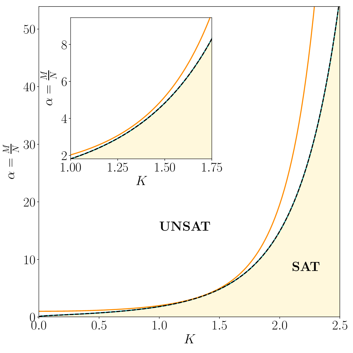
We plotted the annealed capacity, the replica symmetric capacity and the AT-line for the step, rectangle and $u$ -function binary perceptrons as functions of $K$ in fig. 4, 5, 6.

IV.3.1 Step binary perceptron

We note that for the step binary perceptron the RS solution is always stable towards 1RSB, even for negative threshold $K<0$ . This is interesting in the view of recent work on the spherical perceptron with negative threshold where the replica symmetry breaks for all $K<0$ , and full-step RSB is needed to evaluate the storage capacity 20.

IV.3.2 Rectangle

As the RS capacity $\alpha_{\rm RS}^{r}$ is always below the AT line $\alpha_{\rm AT}^{r}$ , the RS solution is always locally stable.

IV.3.3 $u$ -function

There is a crossing between the values of the RS capacity $\alpha_{\rm RS}^{u}$ and the AT-line $\alpha_{\rm AT}^{u}$ , which defines implicitly the value $K^{*}\simeq 0.817$ , and matches the equality in eq. (10):

\frac{-\log\left(2\right)}{\log\left(p_{u,K^{*}}\right)}=\frac{\pi}{2}\frac{\left(p_{u,K^{*}}\right)^{2}}{e^{-(K^{*})^{2}}(K^{*})^{2}}\,.

(17)

For $K\leq K^{*}$ , the RS solution is locally stable, while for $K>K^{*}$ the RS solution becomes unstable, and a symmetry breaking solution appears.

IV.4 1RSB calculation

In the previous section we concluded that the replica symmetric solution is unstable in the $u-$ function binary perceptron for $K>K^{*}$ , we analyze therefore the first-step of replica symmetry breaking (1RSB) ansatz in this section. This ansatz and calculations is due to seminal works of G. Parisi and is classic in the field of disordered systems and well presented in the literature 13; parisi1979infinite; parisi1980sequence; parisi1980order, we thus mainly give the key formulas and defer the details into the Appendix VI.3.

The 1RSB ansatz assumes that the space of configurations splits into states. Consequently replicas are not symmetric anymore and instead $n$ replicas are organized in $\frac{n}{m}$ groups containing $m$ replicas each:

\forall(a,b)\in[1:n]\times[1:n],\hskip 2.84544pt\frac{1}{N}({\mathbb{w}}^{a}\cdot{\mathbb{w}}^{b})=\begin{cases}q_{1}\textrm{ if $a$,$b$ belong to the same state,}\\ q_{0}\textrm{ if $a$,$b$ do not belong to the same state,}\\ Q=1\textrm{ if }a=b\,.\end{cases}

(18)

Following 25, the partition function $\mathcal{Z}_{m}$ associated to $m$ replicas falling in the same state is expressed as a sum over all possible states $\Psi$ weighted by their corresponding free entropy $\phi$ :

\mathcal{Z}_{m}=\sum_{\{\Psi\}}\exp(Nm\phi(\Psi))=\sum_{\{\phi\}}{\cal N}_{\phi}\exp(Nm\phi)=\sum_{\{\phi\}}\exp(N\Sigma(\phi))\exp(Nm\phi)\sim\int d\phi\exp(N(m\phi+\Sigma(\phi))\,,

where we introduced the number of states at a given free entropy $\phi$ : ${\cal N}_{\phi}\equiv\exp(N\Sigma(\phi))$ and the complexity $\Sigma(\phi)$ , also called the configurational entropy.

Using the saddle point method in the $N\to\infty$ limit, the 1RSB replicated free entropy $\Phi_{\rm 1RSB}$ is written as a function of the Parisi parameter $m$ , the free entropy $\phi$ and the complexity $\Sigma(\phi)$ :

\Phi_{\rm 1RSB}(m,\alpha)\equiv\lim_{N\to\infty}\frac{1}{N}\mathbb{E}_{{\mathbb{X}}}\left[\log(\mathcal{Z}_{m}({\mathbb{X}}))\right]=m\phi+\Sigma(\phi)\,.

(19)

Injecting the 1RSB ansatz eq. (18) in the replica derivation eq. (14), the 1RSB replicated free entropy $\Phi_{\rm 1RSB}$ is written as a saddle point equation over ${\mathbb{q}}=(q_{0},q_{1})$ and ${\mathbb{\hat{q}}}=(\hat{q}_{0},\hat{q}_{1})$ (see Appendix VI.3):

\Phi_{\rm 1RSB}(m,\alpha)=\underset{{\mathbb{q}},{\mathbb{\hat{q}}}}{\textrm{extr}}\left\{\frac{m}{2}\left(q_{1}\hat{q}_{1}-1\right)+\frac{m^{2}}{2}\left(q_{0}\hat{q}_{0}-q_{1}\hat{q}_{1}\right)+m\mathcal{I}^{w}_{\rm 1RSB}({\mathbb{\hat{q}}})+\alpha m\mathcal{I}^{z}_{\rm 1RSB}({\mathbb{q}})\right\}

(20)

\textrm{ with }\begin{cases}\mathcal{I}^{w}_{\rm 1RSB}({\mathbb{\hat{q}}})=\frac{1}{m}\int Dt_{0}\log\left(\int Dt_{1}g_{0}^{w}\left({\mathbb{t}},{\mathbb{\hat{q}}}\right)^{m}\right)\,,\vskip 8.5359pt\\ \mathcal{I}^{z}_{\rm 1RSB}({\mathbb{q}})=\frac{1}{m}\int Dt_{0}\log\left(\int Dt_{1}f_{0}^{z}\left({\mathbb{t}},{\mathbb{q}}\right)^{m}\right)\,,\end{cases}

\textrm{denoting ${\mathbb{t}}=(t_{0},t_{1})$, and for $i\in\mathbbm{N}$: }\begin{cases}g_{i}^{w}({\mathbb{t}},{\mathbb{\hat{q}}})=\int dw\,w^{i}P_{w}(w)\exp\left(\frac{(1-\hat{q}_{1})}{2}w^{2}+\left(\sqrt{\hat{q}_{0}}t_{0}+\sqrt{\hat{q}_{1}-\hat{q}_{0}}t_{1}\right)w\right)\,,\vskip 8.5359pt\\ f_{i}^{z}({\mathbb{t}},{\mathbb{q}})=\int Dz\,z^{i}\varphi(\sqrt{q_{0}}t_{0}+\sqrt{q_{1}-q_{0}}t_{1}+\sqrt{1-q_{1}}z)\,.\end{cases}

(21)

Taking the derivative of $\Phi_{\rm 1RSB}$ with respect to $m$ , the free entropy $\phi$ and complexity $\Sigma$ can be written as:

\begin{cases}\phi(\alpha)=\frac{\partial\Phi_{\rm 1RSB}(m,\alpha)}{\partial m}=\underset{{\mathbb{q}},{\mathbb{\hat{q}}}}{\textrm{extr}}\left\{\frac{1}{2}(q_{1}\hat{q}_{1}-1)+m\left(q_{0}\hat{q}_{0}-q_{1}\hat{q}_{1}\right)+\mathcal{J}^{w}_{\rm 1RSB}({\mathbb{\hat{q}}})+\alpha\mathcal{J}^{z}_{\rm 1RSB}({\mathbb{q}})\right\}\,,\vskip 8.5359pt\\ \Sigma(\phi)=\Phi_{\rm 1RSB}-m\phi=\underset{{\mathbb{q}},{\mathbb{\hat{q}}}}{\textrm{extr}}\left\{\frac{m^{2}}{2}(q_{1}\hat{q}_{1}-q_{0}\hat{q}_{0})+m(\mathcal{I}^{w}_{\rm 1RSB}-\mathcal{J}^{w}_{\rm 1RSB})({\mathbb{\hat{q}}})+m\alpha(\mathcal{I}^{z}_{\rm 1RSB}-\mathcal{J}^{z}_{\rm 1RSB})({\mathbb{q}})\right\}\,,\end{cases}

(22)

\textrm{ with }\begin{cases}\mathcal{J}^{w}_{\rm 1RSB}({\mathbb{\hat{q}}})=\frac{\partial\left(m\mathcal{I}^{w}_{\rm 1RSB}\right)}{\partial m}=\int Dt_{0}\frac{\int Dt_{1}\log\left(g_{0}^{w}({\mathbb{t}},{\mathbb{\hat{q}}})\right)g_{0}^{w}({\mathbb{t}},{\mathbb{\hat{q}}})^{m}}{\int Dt_{1}g_{0}^{w}({\mathbb{t}},{\mathbb{\hat{q}}})^{m}}\,,\vskip 5.69046pt\\ \mathcal{J}^{z}_{\rm 1RSB}({\mathbb{q}})=\frac{\partial\left(m\mathcal{I}^{z}_{\rm 1RSB}\right)}{\partial m}=\int Dt_{0}\frac{\int Dt_{1}\log\left(f_{0}^{z}({\mathbb{t}},{\mathbb{q}})\right)f_{0}^{z}({\mathbb{t}},{\mathbb{q}})^{m}}{\int Dt_{1}f_{0}^{z}({\mathbb{t}},{\mathbb{q}})^{m}}\,.\vskip 5.69046pt\\ \end{cases}

IV.5 1RSB results for UBP

From now on, we only consider the $u-$ function binary perceptron, whose RS solution is unstable for $K>K^{*}$ . To describe the equilibrium of the system in the SAT phase, we need to find the value of the Parisi parameter at equilibrium $m_{\rm eq}$ . The complexity $\Sigma(\phi)$ is the entropy of clusters having internal entropy $\phi$ . In order to capture clusters that carry almost all configurations, we need to maximize the total entropy $\phi_{\rm tot}=\Sigma(\phi)+\phi$ under the constraint that the free entropy and complexity are both positive $\phi\geq 0$ and $\Sigma(\phi)\geq 0$ . Hence from eq. (19), the equilibrium Parisi parameter $m_{\rm eq}$ verifies

\phi_{\rm eq}=\underset{\phi\geq 0,\Sigma\geq 0}{\textrm{argmax }}{\{\phi+\Sigma(\phi)\}}\hskip 28.45274pt\textrm{and}\hskip 28.45274ptm_{\rm eq}=\left.-\frac{d\Sigma}{d\phi}\right|_{\phi_{\rm eq}}\,.

Using the expressions eq. (22) and varying the Parisi parameter $m\in[0;1]$ , we obtain the curve of the complexity $\Sigma(\phi)$ as shown in fig. 7. At $m=1$ , the complexity is negative. Decreasing $m$ , the complexity increases and becomes positive at the value $m_{\rm eq}$ . Besides for small values of $m$ , an unphysical (convex) branch appears, as commonly observed in other systems solved by the replica method.

We note that at $\alpha$ increases both the equilibrium complexity and free entropy decrease. In constraint satisfaction problems such as K-satisfiability or random graph coloring the mechanism in which the satisfiability threshold appears is that the maximum of the complexity becomes negative. In the present UBP problem it is actually both the free entropy and the complexity that vanish together, as illustrated in fig. 7.

Computing the equilibrium value $m_{\rm eq}(\alpha)$ , we have access to the corresponding equilibrium overlaps $q_{0}^{*}$ and $q_{1}^{*}$ , that we may compare with the RS solution $q_{\rm RS}$ . All these are depicted in fig. 8. The function $m_{\rm eq}(\alpha)$ shows a non monotonic behaviour as it has been previously observed, e.g. in the Sherrington-Kirkpatrick model as a function of temperature Mezard1987.

We also compute the 1RSB entropy that verifies $\phi_{\rm 1RSB}^{u}\leq\phi_{\rm RS}^{u}$ and which vanishes at the 1RSB capacity $\alpha_{\rm 1RSB}^{u}$ as depicted in fig. 9a. We note that the above inequality is as predicted by Parisi’s replica theory Mezard1987, taking into account that we are working at strictly zero energy, where the entropy becomes minus the free energy.

The 1RSB solution provides a small correction to the RS result for storage capacity, as illustrated in fig. 9b, where we plotted the difference between the annealed upper bound and the capacity for the RS and 1RSB solutions: $\alpha_{a}^{u}-\alpha_{\rm RS}^{u}$ and $\alpha_{a}^{u}-\alpha_{\rm 1RSB}^{u}$ .

IV.6 1RSB Stability

In the previous section we evaluated the 1RSB storage capacity of the $u-$ function binary perceptron for $K>K^{*}$ . In this section we will argue that this cannot be an exact solution to the problem.

We could investigate the stability of 1RSB towards further levels of replica symmetry breaking along the same lines we did for the RS solution. However, in the present case we do not need to do that to see that the obtained solution cannot be correct. The explanations lies in the breaking of the up-down symmetry in the problem. This symmetry must either be broken explicitly as in the ferromagnet, where the system would acquire an overall magnetization, but we have not observed any trace of this in the present problem. Or this up-down symmetry must be conserved in the final correct solution. The conservation of the up-down symmetry is manifested in the value $q_{0}=0$ in the replica symmetric phase. The fact that in the 1RSB solution evaluated above we do not observe $q_{0}=0$ , but instead $q_{0}>0$ is a sign of the fact that we are evaluating a wrong solution. The only possible way to obtain an exact solution we foresee is to evaluate the full-step replica symmetry breaking with a continuity of overlaps $q(x)$ , the smallest one of them should be $0$ in order to restore the up-down symmetry. We let the evaluation of the full-RSB for future work.

Finally let us note that the 1RSB solution obtained in the previous section can be interpreted as frozen-2RSB. In 2RSB we would have 3 kinds of overlaps, $q_{0}$ , $q_{1}$ and $q_{2}$ . In frozen 2RSB we would have $q_{2}=1$ , $q_{1}=q_{1}^{\rm 1RSB}$ , $q_{0}=q_{0}^{\rm 1RSB}$ .

V Conclusion

The step-function binary perceptron has thus far eluded a rigorous establishment of the conjectured storage capacity, eq. (2). This prediction is expected to be exact because of the frozen-1RSB nature of the problem 2; 16. At the same time the work of baldassi2015subdominant sheds light on the fact that the structure of the space of solutions is not fully described by the frozen-1RSB picture, and that rare dense and unfrozen regions exist and in fact are amenable to dynamical procedures searching for solutions. It remains to be understood how is it possible that the 1RSB calculation does not capture these dense unfrozen regions of solutions baldassi2015subdominant. They do not dominate the equilibrium, but the RSB calculation is expected to describe rare events via their large deviations, which in this case it does not.

In this paper we focus on two cases of the binary perceptron with symmetric constraints, the rectangle binary perceptron and the $u-$ function binary perceptron. We prove (up to a numerical assumption) using the second moment method that the storage capacity agrees in those cases with the annealed upper bound, except for the $u-$ function binary perceptron for $K>K^{*}$ eq. (5). We analyze the 1RSB solution in that case and indeed obtain a lower prediction for the storage capacity. However, we do not expect the 1RSB to provide the exact solution because it does not respect the up-down symmetry of the problem. Though the precise nature of the satisfiable phase for the $u-$ function binary perceptron for $K>K^{*}$ remains illusive, we can conjecture it is full-RSB parisi1979infinite; parisi1980sequence; parisi1980order. Establishing this rigorously would provide much deeper understanding and remains a challenging subject for future work.

Acknowledgement

We thank Florent Krzakala, Joe Neeman, and Pierfrancesco Urbani for useful discussions. We acknowledge funding from the ERC under the European Unionâs Horizon 2020 Research and Innovation Programme Grant Agreement 714608-SMiLe. WP was supported in part by EPSRC grant EP/P009913/1.

References

[1] E. Gardner & B. Derrida. Optimal storage properties of neural network models. J. Phys. A: Math. and Gen, 1988.
[2] W. Krauth & M. Mézard. Storage capacity of memory networks with binary couplings. J. Phys. France, 1989.
[3] Timothy LH Watkin, Albrecht Rau, and Michael Biehl. The statistical mechanics of learning a rule. Reviews of Modern Physics, 65(2):499, 1993.
[4] HS Seung, Haim Sompolinsky, and N Tishby. Statistical mechanics of learning from examples. Physical Review A, 45(8):6056, 1992.
[5] A. Engel & C. Van den Broeck. Statistical mechanics of learning. Cambridge university press, 2001.
[6] H. Nishimori. Statistical Physics of Spin Glasses and Information Processing: An Introduction. Oxford University Press, Oxford, UK, 2001.
[7] Michel Talagrand. The Parisi formula. Annals of mathematics, pages 221–263, 2006.
[8] Michel Talagrand. Spin glasses: a challenge for mathematicians: cavity and mean field models, volume 46. Springer Science & Business Media, 2003.
[9] M. Mézard & A. Montanari. Information, Physics, and Computation. Oxford Graduate Texts, 2009.
[10] Dimitris Achlioptas, Amin Coja-Oghlan, and Federico Ricci-Tersenghi. On the solution-space geometry of random constraint satisfaction problems. Random Structures & Algorithms, 38(3):251–268, 2011.
[11] Dmitry Panchenko. The Parisi formula for mixed $p$ -spin models. The Annals of Probability, 42(3):946–958, 2014.
[12] Jian Ding, Allan Sly, and Nike Sun. Proof of the satisfiability conjecture for large k. In Proceedings of the forty-seventh annual ACM symposium on Theory of computing, pages 59–68. ACM, 2015.
[13] Jeong Han Kim and James R Roche. Covering cubes by random half cubes, with applications to binary neural networks. Journal of Computer and System Sciences, 56(2):223–252, 1998.
[14] Mihailo Stojnic. Discrete perceptrons. arXiv preprint arXiv:1306.4375, 2013.
[15] Jian Ding and Nike Sun. Capacity lower bound for the Ising perceptron. arXiv preprint arXiv:1809.07742, 2018.
[16] Nikhil Bansal and Joel H. Spencer. On-line balancing of random inputs. arXiv preprint arXiv:1903.06898, 2019.
[17] Manfred Opper. Statistical physics estimates for the complexity of feedforward neural networks. Physical Review E, 51(4):3613, 1995.
[18] Geert Jan Bex, Roger Serneels, and Christian Van den Broeck. Storage capacity and generalization error for the reversed-wedge ising perceptron. Physical Review E, 51(6):6309, 1995.
[19] Tadaaki Hosaka, Yoshiyuki Kabashima, and Hidetoshi Nishimori. Statistical mechanics of lossy data compression using a nonmonotonic perceptron. Physical Review E, 66(6):066126, 2002.
[20] S. Franz, G. Parisi, M. Sevelev, P. Urbani, and F. Zamponi. Universality of the SAT-UNSAT (jamming) threshold in non-convex continuous constraint satisfaction problems. SciPost Phys, 2017.
[21] Giorgio Parisi. Infinite number of order parameters for spin-glasses. Physical Review Letters, 43(23):1754, 1979.
[22] Giorgio Parisi. A sequence of approximated solutions to the sk model for spin glasses. Journal of Physics A: Mathematical and General, 13(4):L115, 1980.
[23] Giorgio Parisi. The order parameter for spin glasses: a function on the interval 0-1. Journal of Physics A: Mathematical and General, 13(3):1101, 1980.
[24] James G Wendel. A problem in geometric probability. Math. Scand, 11:109–111, 1962.
[25] Thomas M Cover. Geometrical and statistical properties of systems of linear inequalities with applications in pattern recognition. IEEE transactions on electronic computers, (3):326–334, 1965.
[26] Mariya Shcherbina and Brunello Tirozzi. Rigorous solution of the Gardner problem. Communications in mathematical physics, 234(3):383–422, 2003.
[27] Mihailo Stojnic. Another look at the Gardner problem. arXiv preprint arXiv:1306.3979, 2013.
[28] Silvio Franz and Giorgio Parisi. The simplest model of jamming. Journal of Physics A: Mathematical and Theoretical, 49(14):145001, 2016.
[29] Mihailo Stojnic. Negative spherical perceptron. arXiv preprint arXiv:1306.3980, 2013.
[30] Dimitris Achlioptas and Cristopher Moore. The asymptotic order of the random k-SAT threshold. In Foundations of Computer Science, 2002. Proceedings. The 43rd Annual IEEE Symposium on, pages 779–788. IEEE, 2002.
[31] K.Y.M Wong & Y. Kabashima H. Huang. Entropy landscape of solutions in the binary perceptron problem. Journal of Physics A: Mathematical and Theoretical, 2013.
[32] Haiping Huang and Yoshiyuki Kabashima. Origin of the computational hardness for learning with binary synapses. Physical Review E, 90(5):052813, 2014.
[33] Lenka Zdeborová and Marc Mézard. Constraint satisfaction problems with isolated solutions are hard. Journal of Statistical Mechanics: Theory and Experiment, 2008(12):P12004, 2008.
[34] Alfredo Braunstein and Riccardo Zecchina. Learning by message passing in networks of discrete synapses. Physical review letters, 96(3):030201, 2006.
[35] Carlo Baldassi, Alessandro Ingrosso, Carlo Lucibello, Luca Saglietti, and Riccardo Zecchina. Subdominant dense clusters allow for simple learning and high computational performance in neural networks with discrete synapses. Physical review letters, 115(12):128101, 2015.
[36] Carlo Baldassi, Christian Borgs, Jennifer T Chayes, Alessandro Ingrosso, Carlo Lucibello, Luca Saglietti, and Riccardo Zecchina. Unreasonable effectiveness of learning neural networks: From accessible states and robust ensembles to basic algorithmic schemes. Proceedings of the National Academy of Sciences, 113(48):E7655–E7662, 2016.
[37] Lenka Zdeborová and Marc Mézard. Locked constraint satisfaction problems. Physical review letters, 101(7):078702, 2008.
[38] Lenka Zdeborová and Florent Krzakala. Quiet planting in the locked constraint satisfaction problems. SIAM Journal on Discrete Mathematics, 25(2):750–770, 2011.
[39] Dimitris Achlioptas and Amin Coja-Oghlan. Algorithmic barriers from phase transitions. In Foundations of Computer Science, 2008. FOCS’08. IEEE 49th Annual IEEE Symposium on, pages 793–802. IEEE, 2008.
[40] Florent Krzakala and Lenka Zdeborová. Hiding quiet solutions in random constraint satisfaction problems. Physical review letters, 102(23):238701, 2009.
[41] Elchanan Mossel, Joe Neeman, and Allan Sly. Reconstruction and estimation in the planted partition model. Probability Theory and Related Fields, 162(3-4):431–461, 2015.
[42] Amin Coja-Oghlan, Florent Krzakala, Will Perkins, and Lenka Zdeborová. Information-theoretic thresholds from the cavity method. Advances in Mathematics, 333:694–795, 2018.
[43] Ehud Friedgut. Sharp thresholds of graph properties, and the k-SAT problem. Journal of the American mathematical Society, 12(4):1017–1054, 1999.
[44] OC Martin, M Mézard, and O Rivoire. Frozen glass phase in the multi-index matching problem. Physical review letters, 93(21):217205, 2004.
[45] C. Schülke. Statistical physics of linear and bilinear inference problems. PhD thesis, Université Paris Diderot - La Sapienza, 2016.
[46] J.R.L de Almeida and D.J Thouless. Stability of the Sherrington-Kirkpatrick solution of a spin glass model. J. Phys. A: Math. Gen, 1978.
[47] & M.Virasoro M.Mézard, G.Parisi. Spin glasses and beyond. World Science, Singapore, 1987.
[48] R. Monasson. Structural glass transition and the entropy of the metastable states. Physical Review Letter, (75 2847), 1995.
[49] Marc Mezard, Giorgio Parisi, and Miguel Angel Virasoro. Spin Glass Theory and Beyond, 1987.

VI Appendices

VI.1 General replica calculation

We present here the replica computation for general prior distribution $P_{w}$ and constraint function $\varphi$ . In order to compute the quenched average of the free entropy, we consider the partition function of $n\in\mathbb{N}$ identical copies of the initial system. Using the replica trick, and an analytical continuation, the averaged free entropy $\phi$ of the initial system reads:

\displaystyle\phi(\alpha)

\displaystyle\equiv\lim_{N\rightarrow+\infty}\frac{1}{N}\mathbb{E}_{{\mathbb{X}}}[\log(\mathcal{Z({\mathbb{X}})})]=\lim_{N\rightarrow+\infty}\lim_{n\rightarrow 0}\frac{1}{N}\frac{\partial\log\left(\mathbb{E}_{{\mathbb{X}}}[\mathcal{Z}({\mathbb{X}})^{n}]\right)}{\partial n}\,,

(23)

where the replicated partition function can be written as

\displaystyle\mathbb{E}_{{\mathbb{X}}}[\mathcal{Z}({\mathbb{X}})^{n}]

\displaystyle=\int d{\mathbb{X}}P_{X}({\mathbb{X}})\mathcal{Z}({\mathbb{X}})^{n}=\int d{\mathbb{X}}P_{X}({\mathbb{X}})\prod_{a=1}^{n}\int d{\mathbb{w}}^{a}P_{w}({\mathbb{w}}^{a})\int d{\mathbb{z}}^{a}\mathcal{C}({\mathbb{z}}^{a})\delta({\mathbb{z}}^{a}-{\mathbb{X}}{\mathbb{w}}^{a})\,,

(24)

with the global constraint function $\mathcal{C}({\mathbb{z}})=\displaystyle\prod_{\mu=1}^{M}\varphi(z_{\mu})$ .

We suppose that inputs are $iid$ distributed from $P_{X}\triangleq\mathcal{N}\left(0,\frac{1}{N}\right)$ . More precisely, for $i,j\in[1:N]$ , $\mu,\nu\in[1:M]$ , $\mathbb{E}_{\mathbb{X}}[X_{i\mu}X_{j\nu}]=\frac{1}{N}\delta_{\mu\nu}\delta_{ij}$ . Hence $z_{\mu}^{a}=\sum_{i=1}^{N}X_{i\mu}w_{i}^{a}$ is the sum of $iid$ random variables. The central limit theorem insures that $z_{\mu}^{a}\sim\mathcal{N}\left(\mathbb{E}_{{\mathbb{X}}}[z_{\mu}^{a}],\mathbb{E}_{{\mathbb{X}}}[z_{\mu}^{a}z_{\mu}^{b}]\right)$ , with two first moments:

\begin{cases}\mathbb{E}_{{\mathbb{X}}}[z_{\mu}^{a}]=\sum_{i=1}^{N}\mathbb{E}_{{\mathbb{X}}}[X_{i\mu}]w_{i}^{a}=0\\ \mathbb{E}_{{\mathbb{X}}}[z_{\mu}^{a}z_{\mu}^{b}]=\sum_{ij}\mathbb{E}_{{\mathbb{X}}}[X_{i\mu}X_{j\mu}]w_{i}^{a}w_{j}^{b}=\frac{1}{N}\sum_{ij}\delta_{ij}w_{i}^{a}w_{j}^{b}=\frac{1}{N}\sum_{i=1}^{N}w_{i}^{a}w_{i}^{b}\,.\end{cases}

(25)

In the following we introduce the symmetric overlap matrix ${\mathbb{Q}}\equiv(\frac{1}{N}\sum_{i=1}^{N}w_{i}^{a}w_{i}^{b})_{a,b=1..n}$ . Define ${\mathbb{\tilde{z}}}_{\mu}\equiv(z^{a}_{\mu})_{a=1..n}$ and ${\mathbb{\tilde{w}}}_{i}\equiv(w_{i}^{a})_{a=1..n}$ . ${\mathbb{\tilde{z}}}_{\mu}$ follows a multivariate gaussian distribution ${\mathbb{\tilde{z}}}_{\mu}\sim P_{\tilde{z}}\triangleq\mathcal{N}({\mathbb{0}},{\mathbb{Q}})$ and $P_{\tilde{w}}({\mathbb{\tilde{w}}})=\prod_{a=1}^{n}[\delta(\tilde{w}_{a}-1)+\delta(\tilde{w}_{a}+1)]$ . Introducing the change of variable and the Fourier representation of the $\delta$ -Dirac function that involves a new parameter ${\mathbb{\hat{Q}}}$ :

1=\int d{\mathbb{Q}}\prod_{a\leq b}\delta\left(NQ_{ab}-\sum_{i=1}^{N}w_{i}^{a}w_{i}^{b}\right)=\int d{\mathbb{Q}}\int d{\mathbb{\hat{Q}}}\exp\left(-\frac{N}{2}\\ Tr({\mathbb{Q\hat{Q}}})\right)\exp\left(\frac{1}{2}\sum_{i=1}^{N}{\mathbb{\tilde{w}}}_{i}^{\intercal}{\mathbb{\hat{Q}}}{\mathbb{\tilde{w}}}_{i}\right),

the replicated partition function becomes an integral over the matrix parameters ${\mathbb{Q}}$ and ${\mathbb{\hat{Q}}}$ , that can be evaluated using Laplace method in the $N\to\infty$ limit,

	$\displaystyle\mathbb{E}_{{\mathbb{X}}}[\mathcal{Z}({\mathbb{X}})^{n}]$	$\displaystyle=\int d{\mathbb{Q}}d{\mathbb{\hat{Q}}}e^{-N\left(\frac{1}{2}{\rm Tr}({\mathbb{Q\hat{Q}}})-\log\left(\int d{\mathbb{\tilde{w}}}P_{\tilde{w}}({\mathbb{\tilde{w}}})e^{\frac{1}{2}{\mathbb{\tilde{w}}}^{\intercal}{\mathbb{\hat{Q}}}{\mathbb{\tilde{w}}}}\right)-\alpha\log\left(\int d{\mathbb{\tilde{z}}}P_{\tilde{z}}({\mathbb{\tilde{z}}})\mathcal{C}({\mathbb{\tilde{z}}})\right)\right)}$		(26)
		$\displaystyle=\int d{\mathbb{Q}}d{\mathbb{\hat{Q}}}e^{-NS_{n}({\mathbb{Q}},{\mathbb{\hat{Q}}})}\underset{N\to\infty}{\simeq}e^{-N\cdot\text{SP}_{{\mathbb{Q}},{\mathbb{\hat{Q}}}}\left\{S_{n}({\mathbb{Q}},{\mathbb{\hat{Q}}})\right\}},$		(27)

where SP states for saddle point and we defined

\begin{cases}S_{n}({\mathbb{Q}},{\mathbb{\hat{Q}}})=\frac{1}{2}{\rm Tr}({\mathbb{Q\hat{Q}}})-\log(\mathcal{I}^{w}_{n}({\mathbb{\hat{Q}}}))-\alpha\log\left(\mathcal{I}^{z}_{n}({\mathbb{Q}})\right)\vskip 5.69046pt\\ \mathcal{I}^{w}_{n}({\mathbb{\hat{Q}}})=\int_{\mathbb{R}^{n}}d{\mathbb{\tilde{w}}}P_{\tilde{w}}({\mathbb{\tilde{w}}})e^{\frac{1}{2}{\mathbb{\tilde{w}}}^{\intercal}{\mathbb{\hat{Q}}}{\mathbb{\tilde{w}}}}\vskip 5.69046pt\\ \mathcal{I}^{z}_{n}({\mathbb{Q}})=\int_{\mathbb{R}^{n}}d{\mathbb{\tilde{z}}}P_{\tilde{z}}({\mathbb{\tilde{z}}})\mathcal{C}({\mathbb{\tilde{z}}}).\end{cases}

(28)

Finally, using eq. (23) and switching the two limits $n\to 0$ and $N\to\infty$ , the quenched free entropy $\phi$ simplifies as a saddle point equation

\phi(\alpha)=-\text{SP}_{{\mathbb{Q}},{\mathbb{\hat{Q}}}}\left\{\lim_{n\rightarrow 0}\frac{\partial S_{n}(\mathbb{Q},\mathbb{\hat{Q}})}{\partial n}\right\},

(29)

over general symmetric matrices ${\mathbb{Q}}$ and ${\mathbb{\hat{Q}}}$ . In the following we will assume simple ansatz for these matrices that allows to get analytic expressions in $n$ in order to take the derivative.

VI.2 RS entropy

Let’s compute the functional $S_{n}({\mathbb{Q}},{\mathbb{\hat{Q}}})$ appearing in the free entropy eq. (29) in the simplest ansatz: the Replica Symmetric ansatz. This later assumes that all replica remain equivalent with a common overlap $q_{0}=\frac{1}{N}\sum_{i=1}^{N}w_{i}^{a}w_{i}^{b}$ for $a\neq b$ and a norm $Q=\frac{1}{N}\sum_{i=1}^{N}w_{i}^{a}w_{i}^{a}$ , leading to the following expressions of the matrices ${\mathbb{Q}}$ and ${\mathbb{\hat{Q}}}\in\mathbb{R}^{n\times n}$ :

\begin{aligned} {\mathbb{Q}}=\begin{pmatrix}Q&q_{0}&...&q_{0}\\ q_{0}&Q&...&...\\ ...&...&...&q_{0}\\ q_{0}&...&q_{0}&Q\\ \end{pmatrix}\end{aligned}\hskip 14.22636pt\textrm{ and }\hskip 14.22636pt\begin{aligned} {\mathbb{\hat{Q}}}=\begin{pmatrix}\hat{Q}&\hat{q}_{0}&...&\hat{q}_{0}\\ \hat{q}_{0}&\hat{Q}&...&...\\ ...&...&...&\hat{q}_{0}\\ \hat{q}_{0}&...&\hat{q}_{0}&\hat{Q}\\ \end{pmatrix}.\end{aligned}

(30)

Let’s compute separately the terms involved in the functional $S_{n}({\mathbb{Q}},{\mathbb{\hat{Q}}})$ eq. (28): the first is a trace term, the second a term of prior $\mathcal{I}^{w}_{n}$ and finally the third a term depending on the constraint $\mathcal{I}^{z}_{n}$ .

Trace term

The trace term can be easily computed and takes the following form:

\left.\frac{1}{2}{\rm Tr}({\mathbb{Q\hat{Q}}})\right|_{\rm RS}=\frac{1}{2}\left(nQ\hat{Q}+n(n-1)q_{0}\hat{q}_{0}\right).

(31)

Prior integral

Evaluated at the RS fixed point, and using a gaussian identity also known as a Hubbard-Stratonovich transformation, the prior integral can be further simplified

	$\displaystyle\left.\mathcal{I}^{w}_{n}({\mathbb{\hat{Q}}})\right\|_{\rm RS}$	$\displaystyle=\int d{\mathbb{\tilde{w}}}P_{\tilde{w}}({\mathbb{\tilde{w}}})e^{\frac{1}{2}{\mathbb{\tilde{w}}}^{\intercal}{\mathbb{\hat{Q}}}{\mathbb{\tilde{w}}}}=\int d{\mathbb{\tilde{w}}}P_{\tilde{w}}({\mathbb{\tilde{w}}})\exp{\left({\frac{(\hat{Q}-\hat{q}_{0})}{2}\sum_{a=1}^{n}(\tilde{w}^{a})^{2}}\right)}\exp{\left(\hat{q}_{0}\left(\sum_{a=1}^{n}\tilde{w}^{a}\right)^{2}\right)}$		(32)
		$\displaystyle=\int Dt\left[\int dwP_{w}(w)\exp{\left({\frac{(\hat{Q}-\hat{q}_{0})}{2}w^{2}}+t\sqrt{\hat{q}_{0}}w\right)}\right]^{n}.$		(33)

Constraint integral

Recall the vector ${\mathbb{\tilde{z}}}\sim P_{\tilde{z}}\triangleq\mathcal{N}({\mathbb{0}},{\mathbb{Q}})$ follows a gaussian distribution with zero mean and covariance matrix ${\mathbb{Q}}$ . In the RS ansatz, the covariance can be rewritten as a linear combination of the identity ${\mathbb{I}}$ and ${\mathbb{J}}$ the matrix with all ones entries of size $n\times n$ : $\left.{\mathbb{Q}}\right|_{\rm RS}=(Q-q_{0}){\mathbb{I}}+q_{0}{\mathbb{J}}$ , that allows to split the variable $z^{a}=\sqrt{q_{0}}t+\sqrt{Q-q_{0}}u^{a}$ with $t\sim\mathcal{N}(0,1)$ and $\forall a,~u_{a}\sim\mathcal{N}(0,1)$ . Finally, the constraint integral reads:

	$\displaystyle\left.\mathcal{I}^{z}_{n}({\mathbb{Q}})\right\|_{\rm RS}$	$\displaystyle=\int d{\mathbb{\tilde{z}}}P_{\tilde{z}}({\mathbb{\tilde{z}}})\mathcal{C}({\mathbb{\tilde{z}}})=\int Dt\int\prod_{a=1}^{n}Du^{a}\varphi\left(\sqrt{q_{0}}t+\sqrt{Q-q_{0}}u^{a}\right)$		(34)
		$\displaystyle=\int Dt\left[\int Du\varphi\left(\sqrt{q_{0}}t+\sqrt{Q-q_{0}}u\right)\right]^{n}.$		(35)

Summary and RS free entropy $\phi_{\rm RS}$

Finally putting pieces together, the functional $S_{n}$ taken at the RS fixed point has an explicit formula and dependency in $n$ :

$\displaystyle\left.S_{n}({\mathbb{Q}},{\mathbb{\hat{Q}}})\right\|_{\rm RS}$	$\displaystyle=\left.\frac{1}{2}{\rm Tr}({\mathbb{Q\hat{Q}}})-\log(\mathcal{I}_{w}^{n}({\mathbb{\hat{Q}}}))-\alpha\log\left(\mathcal{I}_{z}^{n}({\mathbb{Q}})\right)\right\|_{\rm RS}$	(36)
	$\displaystyle\underset{n\to 0}{\simeq}\frac{1}{2}\left(nQ\hat{Q}+n(n-1)q_{0}\hat{q}_{0}\right)-n\int Dt\log\left(\int dwP_{w}(w)\exp{\left({\frac{(\hat{Q}-\hat{q}_{0})}{2}w^{2}}+t\sqrt{\hat{q}_{0}}w\right)}\right)$	(37)
	$\displaystyle-n\alpha\int Dt\log\left(\int Du\varphi\left(y,\sqrt{q_{0}}t+\sqrt{Q-q_{0}}u\right)\right).$	(38)

Finally taking the derivative with respect to $n$ and the $n\to 0$ limit, the RS free entropy has a simple expression

\phi_{\rm RS}(\alpha)=\textrm{SP}_{q_{0},\hat{q}_{0}}\left\{-\frac{1}{2}Q\hat{Q}+\frac{1}{2}q_{0}\hat{q}_{0}+\mathcal{I}^{w}_{\rm RS}(\hat{q}_{0})+\alpha\mathcal{I}^{z}_{\rm RS}(q_{0})\right\},

(39)

with $Q=\hat{Q}=1$ and the following notations,

\begin{cases}\mathcal{I}^{w}_{\rm RS}(\hat{q}_{0})\equiv\int Dt\log\left(\int dwP_{w}(w)\exp{\left({\frac{(\hat{Q}-\hat{q}_{0})}{2}w^{2}}+t\sqrt{\hat{q}_{0}}w\right)}\right)\vskip 14.22636pt\\ \mathcal{I}^{z}_{\rm RS}(q_{0})\equiv\int Dt\log\left(\int Dz\varphi\left(\sqrt{q_{0}}t+\sqrt{Q-q_{0}}z\right)\right)\end{cases}.

(40)

VI.3 1RSB entropy

The free entropy eq. (23) can also be evaluated at the simplest non trivial fixed point: the one step Replica Symmetry Breaking ansatz (1RSB). Instead assuming that replicas are equivalent, it assumes that the symmetry between replica is broken and that replicas are clustered in different states, with inner overlap $q_{1}$ and outer overlap $q_{0}$ . Translating this in a matrix formulation, the matrices can be expressed as

{\mathbb{Q}}=q_{0}{\mathbb{J}}_{n}+\left(q_{1}-q_{0}\right){\mathbb{I}}_{\frac{n}{m}}\otimes{\mathbb{J}}_{m}+\left(Q-q_{1}\right){\mathbb{I}}_{n}\hskip 5.69046pt\textrm{ and }\hskip 5.69046pt{\mathbb{\hat{Q}}}=\hat{q}_{0}{\mathbb{J}}_{n}+\left(\hat{q}_{1}-\hat{q}_{0}\right){\mathbb{I}}_{\frac{n}{m}}\otimes{\mathbb{J}}_{m}+\left(\hat{Q}-\hat{q}_{1}\right){\mathbb{I}}_{n}\,.

(41)

Trace term

Again, the trace term can be easily computed

\left.\frac{1}{2}{\rm Tr}({\mathbb{Q\hat{Q}}})\right|_{\rm 1RSB}=\frac{1}{2}\left(nQ\hat{Q}+n(m-1)q_{1}\hat{q}_{1}+n(n-m)q_{0}\hat{q}_{0}\right).

(42)

Prior integral

Separating replicas with different overlaps, the prior integral can be written as

	$\displaystyle\left.\mathcal{I}^{w}_{n}({\mathbb{\hat{Q}}})\right\|_{\rm 1RSB}$	$\displaystyle=\int d{\mathbb{\tilde{w}}}P_{\tilde{w}}({\mathbb{\tilde{w}}})e^{\frac{(\hat{Q}-\hat{q}_{1})}{2}\sum_{a=1}^{n}(\tilde{w}^{a})^{2}+\frac{(\hat{q}_{1}-\hat{q}_{0})}{2}\sum_{k=1}^{\frac{n}{m}}\sum_{a,b=(k-1)m+1}^{km}\tilde{w}^{a}\tilde{w}^{b}+\frac{\hat{q}_{0}}{2}\left(\sum_{a=1}^{n}\tilde{w}^{a}\right)^{2}}$		(43)
		$\displaystyle=\int Dt_{0}\left[\int Dt_{1}\left[\int dwP_{w}(w)\exp\left(\frac{(\hat{Q}-\hat{q}_{1})}{2}w^{2}+\left(\sqrt{\hat{q}_{0}}t_{0}+\sqrt{\hat{q}_{1}-\hat{q}_{0}}t_{1}\right)w\right)\right]^{m}\right]^{\frac{n}{m}}$		(44)

Constraint integral

Again the vector ${\mathbb{\tilde{z}}}\sim P_{\tilde{z}}\triangleq\mathcal{N}({\mathbb{0}},{\mathbb{Q}})$ follows a gaussian vector with zero mean and covariance $\left.{\mathbb{Q}}\right|_{\rm 1RSB}=q_{0}{\mathbb{J}}_{n}+\left(q_{1}-q_{0}\right){\mathbb{I}}_{\frac{n}{m}}\otimes{\mathbb{J}}_{m}+\left(Q-q_{1}\right){\mathbb{I}}_{n}$ . The gaussian vector of covariance $\left.{\mathbb{Q}}\right|_{\rm 1RSB}$ can be decomposed in a sum of normal gaussian vectors $t_{0}\sim\mathcal{N}(0,1)$ , $\forall k\in[1:\frac{n}{m}],t_{k}\sim\mathcal{N}(0,1)$ and $\forall a\in[(k-1)m+1:km]$ , $u_{a}\sim\mathcal{N}(0,1)$ : $z^{a}=\sqrt{q_{0}}t_{0}+\sqrt{q_{1}-q_{0}}t_{k}+\sqrt{Q-q_{1}}u_{a}$ . Finally the constraint integral reads

	$\displaystyle\left.\mathcal{I}^{z}_{n}({\mathbb{Q}})\right\|_{\rm 1RSB}$	$\displaystyle=\int Dt_{0}\int\prod_{k=1}^{\frac{n}{m}}Dt_{k}\int\prod_{a=(k-1)m+1}^{km}Du_{a}\varphi(\sqrt{q_{0}}t_{0}+\sqrt{q_{1}-q_{0}}t_{k}+\sqrt{Q-q_{1}}u_{a})$		(45)
		$\displaystyle=\int Dt_{0}\left[\int Dt_{1}\left[\int Du\varphi(\sqrt{q_{0}}t_{0}+\sqrt{q_{1}-q_{0}}t_{1}+\sqrt{Q-q_{1}}u)\right]^{m}\right]^{\frac{n}{m}}.$		(46)

Summary and 1RSB free entropy $\phi_{\rm 1RSB}$

Gathering the previous computations eq. (42, 44, 46), the functional $S_{n}$ evaluated at the 1RSB fixed point reads:

$\displaystyle\left.S_{n}({\mathbb{Q}},{\mathbb{\hat{Q}}})\right\|_{\rm 1RSB}$	$\displaystyle=\left.\frac{1}{2}{\rm Tr}({\mathbb{Q\hat{Q}}})-\log(\mathcal{I}_{w}^{n}({\mathbb{\hat{Q}}}))-\alpha\log\left(\mathcal{I}_{z}^{n}({\mathbb{Q}})\right)\right\|_{\rm 1RSB}$	(47)
	$\displaystyle\underset{n\to 0}{\simeq}\frac{1}{2}\left(nQ\hat{Q}+n(m-1)q_{1}\hat{q}_{1}+n(n-m)q_{0}\hat{q}_{0}\right)$	(48)
	$\displaystyle-\frac{n}{m}\int Dt_{0}\log\left(\int Dt_{1}\left[\int d\tilde{w}P_{w}(\tilde{w})\exp\left(\frac{(\hat{Q}-\hat{q}_{1})}{2}\tilde{w}^{2}+\left(\sqrt{\hat{q}_{0}}t_{0}+\sqrt{\hat{q}_{1}-\hat{q}_{0}}t_{1}\right)\tilde{w}\right)\right]^{m}\right)$	(49)
	$\displaystyle-\alpha\frac{n}{m}\int dy\int Dt_{0}\log\left(\int Dt_{1}\left[\int Du\varphi(y,\sqrt{q_{0}}t_{0}+\sqrt{q_{1}-q_{0}}t_{1}+\sqrt{Q-q_{1}}u)\right]^{m}\right).$	(50)

Let’s introduce the replicated free entropy following [48]. We consider $m$ reals replicas of the same system and we imagine we put a small field, that allows the $m$ replicas to fall in the same state. The replicated free entropy is the free entropy corresponding to these $m$ uncorrelated copies in the limit of zero coupling. To compute it, we consider $n^{\prime}=\frac{n}{m}$ replicas. Denoting ${\mathbb{q}}=(q_{0},q_{1})$ and ${\mathbb{\hat{q}}}=(\hat{q}_{0},\hat{q}_{1})$ , the replicated free entropy reads as $m$ times the free entropy of $n$ replicas with 1RSB structure:

$\displaystyle\Phi^{\rm 1RSB}(\alpha):$	$\displaystyle=\left(\lim_{N\to\infty}\frac{1}{N}\mathbb{E}_{{\mathbb{X}}}\left[\log(\mathcal{Z}_{m}({\mathbb{X}})\right]\right)\simeq\lim_{N\to\infty}\frac{1}{N}\lim_{n^{\prime}\rightarrow 0}\frac{\partial\log\left(\mathbb{E}_{{\mathbb{X}}}[\mathcal{Z}^{mn^{\prime}}({\mathbb{X}})]\right)}{\partial n^{\prime}}$	(51)
	$\displaystyle=m\left(\lim_{N\to\infty}\lim_{n\to 0}\frac{1}{N}\frac{\partial\log\left(\mathbb{E}[\mathcal{Z}^{n}({\mathbb{X}})]_{{\mathbb{X}}}\right)}{\partial n}\right)=m\left(-\text{SP}_{{\mathbb{Q}},{\mathbb{\hat{Q}}}}\left\{\lim_{n\rightarrow 0}\frac{\partial S_{n}(\mathbb{Q},\mathbb{\hat{Q}})}{\partial n}\right\}\right)$	(52)
	$\displaystyle=\underset{{\mathbb{q}},{\mathbb{\hat{q}}}}{\textrm{SP}}\left\{\frac{m}{2}\left(q_{1}\hat{q}_{1}-Q\hat{Q}\right)+\frac{m^{2}}{2}\left(q_{0}\hat{q}_{0}-q_{1}\hat{q}_{1}\right)+m\mathcal{I}^{w}_{\rm 1RSB}({\mathbb{\hat{q}}})+\alpha m\mathcal{I}^{z}_{\rm 1RSB}({\mathbb{q}})\right\}\,.$	(53)

with ${\mathbb{t}}=(t_{0},t_{1})$ , $g_{0}^{w}$ and $f_{0}^{z}$ defined in eq. (21) and

\mathcal{I}^{w}_{\rm 1RSB}({\mathbb{\hat{q}}})=\frac{1}{m}\int Dt_{0}\log\left(\int Dt_{1}g_{0}^{w}\left({\mathbb{t}},{\mathbb{\hat{q}}}\right)^{m}\right)\hskip 5.69046pt\textrm{ and }\hskip 5.69046pt\mathcal{I}^{z}_{\rm 1RSB}({\mathbb{q}})=\frac{1}{m}\int Dt_{0}\log\left(\int Dt_{1}f_{0}^{z}\left({\mathbb{t}},{\mathbb{q}}\right)^{m}\right)\,.

(54)

VI.4 RS Stability

VI.4.1 De Almeida Thouless RS Stability

The stability of a given saddle point ansatz is related to the positivity the hessian of the functional $S_{n}$ . This stability analysis has first been done by de Almeida Thouless and following [46, 1, 5], replicons eigenvalues of the RS ansatz $\lambda_{3}^{A}$ and $\lambda_{3}^{B}$ can be expressed as functions of $\{g_{i}^{w},f_{i}^{z}\}_{i=0}^{2}$ defined in eq. (16):

\displaystyle\lambda_{3}^{A}(q_{0})=\frac{1}{(Q-q_{0})^{2}}\int Dt\frac{\left(f_{0}^{z}(f_{0}^{z}-f_{2}^{z})+(f_{1}^{z})^{2}\right)^{2}}{(f_{0}^{z})^{4}}(t,q_{0})\,,\hskip 5.69046pt\textrm{ and }\hskip 5.69046pt\lambda_{3}^{B}(\hat{q}_{0})=\int Dt\frac{\left(g_{0}^{w}g_{2}^{w}-(g_{1}^{w})^{2}\right)^{2}}{(g_{0}^{w})^{4}}(t,\hat{q}_{0})\,.

(55)

The instability AT-line is defined when the determinant of the hessian vanishes that translates as an implicit equation over $\alpha$ , where $q_{0},\hat{q}_{0}$ are solution of the saddle point equations eq. (15) at $\alpha=\alpha_{AT}$ :

\displaystyle\frac{1}{\alpha_{AT}}

\displaystyle=\lambda_{3}^{A}\left(q_{0}(\alpha_{AT}),\beta\right)\lambda_{3}^{B}\left(\hat{q}_{0}(\alpha_{AT})\right)\,.

(56)

However for $\alpha<\alpha_{AT}$ , $(q_{0},\hat{q}_{0})=(0,0)$ is the only solution. Using $\{\tilde{f}^{z}_{i},\tilde{g}^{w}_{i}\}_{i=0}^{2}$ defined eq. (58), this expression simplifies because of the symmetry of the prior distribution $P_{w}$ and the constraints $\varphi$ in the rectangle and $u-$ function cases. In fact the symmetry imposes $\tilde{f}_{1}^{z}=0$ and $\tilde{g}_{1}^{w}=0$ and the condition reads:

\displaystyle\frac{1}{\alpha_{AT}}

\displaystyle=\left(\frac{\tilde{f}_{2}^{z}-\tilde{f}_{0}^{z}}{\tilde{f}_{0}^{z}}\right)^{2}\left(\frac{\tilde{g}_{2}^{w}}{\tilde{g}_{0}^{w}}\right)^{2}\,.

(57)

VI.4.2 Existence and stability of the RS fixed point $(q_{0},\hat{q}_{0})=(0,0)$

We provide an alternative approach to get the instability condition of the RS solution for symmetric prior and constraint. In this symmetric case, the stability can be derived from the existence and stability of the symmetric fixed point $(q_{0},\hat{q}_{0})=(0,0)$ . Let’s define

\displaystyle\begin{cases}F(q_{0})\equiv\alpha\int Dt\frac{(f_{1}^{z})^{2}-2t\sqrt{q_{0}}f_{0}^{z}f_{1}^{z}+q_{0}t^{2}(f_{0}^{z})^{2}}{(1-q_{0})^{2}(f_{0}^{z})^{2}}(t,q_{0})\,,\vskip 8.5359pt\\ G(\hat{q}_{0})\equiv\int Dt\frac{g_{2}^{w}-t\hat{q}_{0}^{-1/2}g_{1}^{w}}{g_{0}^{w}}(t,\hat{q}_{0})\,,\end{cases}\textrm{ with }\begin{cases}\tilde{f}_{i}^{z}(y)\equiv\int Dzz^{i}\varphi(z)\,,\vskip 8.5359pt\\ \tilde{g}_{i}^{w}\equiv\int dww^{i}P_{w}(w)e^{\frac{w^{2}}{2}}\,.\end{cases}

(58)

In fact the saddle point equations at the RS fixed point eq. (15) can be written using the functions $F,G$ , and can be reduced to a single fixed point equation over $q_{0}$ :

\displaystyle\begin{cases}q_{0}=G(\hat{q}_{0})\,,\vskip 8.5359pt\\ \hat{q}_{0}=F(q_{0})\,,\end{cases}\Rightarrow\begin{cases}q_{0}=G\circ F(q_{0})\equiv H(q_{0})\,.\\ \end{cases}

(59)

As stressed above, the RS stability is equivalent to the existence and stability of the fixed point $q_{0}=0$ . According to that, let’s compute the stability of the above fixed point equation eq. (59). Computing $F,F^{\prime},G,G^{\prime}$ in the limit $(q_{0},\hat{q}_{0})\to(0,0)$ , expanding $\{f_{i}^{z}$ , $g_{i}^{w}\}_{i}$ as functions of $\{\tilde{f}^{z}_{i},\tilde{g}^{w}_{i}\}_{i}$ and finally using the symmetry that implies $\tilde{f}_{1}^{z}=0$ and $\tilde{g}_{1}^{w}=0$ :

\begin{cases}F(q_{0})\underset{q_{0}\to 0}{=}\alpha\left[\left(\frac{\tilde{f}_{1}^{z}}{\tilde{f}_{0}^{z}}\right)^{2}+q_{0}\left(\frac{(\tilde{f}_{2}^{z}-\tilde{f}_{0}^{z})^{2}}{(\tilde{f}_{0}^{z})^{2}}+3\frac{(\tilde{f}_{1}^{z})^{4}}{(\tilde{f}_{0}^{z})^{4}}-4\frac{(\tilde{f}_{1}^{z})^{2}(\tilde{f}_{2}^{z}-\tilde{f}_{0}^{z})}{(\tilde{f}_{0}^{z})^{3}}\right)+\mathcal{O}(q_{0}^{2})\right]{\sim}\alpha q_{0}\left(\frac{\tilde{f}_{2}^{z}-\tilde{f}_{0}^{z}}{\tilde{f}_{0}^{z}}\right)^{2}\underset{q_{0}\to 0}{\longrightarrow}0\,,\vskip 5.69046pt\\ \frac{\partial F}{\partial q_{0}}(q_{0})\underset{q_{0}\to 0}{=}\alpha\left[\left(\frac{\tilde{f}_{2}^{z}-\tilde{f}_{0}^{z}}{\tilde{f}_{0}^{z}}\right)^{2}+\left(\frac{\tilde{f}_{1}^{z}}{\tilde{f}_{0}^{z}}\right)^{2}\left(3\frac{(\tilde{f}_{1}^{z})^{2}}{(\tilde{f}_{0}^{z})^{2}}-4\frac{(\tilde{f}_{2}^{z}-\tilde{f}_{0}^{z})}{\tilde{f}_{0}^{z}}\right)+\mathcal{O}(q_{0})\right]\underset{q_{0}\to 0}{\longrightarrow}\alpha\left(\frac{\tilde{f}_{2}^{z}-\tilde{f}_{0}^{z}}{\tilde{f}_{0}^{z}}\right)^{2}\,,\vskip 5.69046pt\\ G(\hat{q}_{0})\underset{\hat{q}_{0}\to 0}{=}\left(\frac{\tilde{g}_{1}^{w}}{\tilde{g}_{0}^{w}}\right)^{2}+\hat{q}_{0}\left(\left(\frac{\tilde{g}_{2}^{w}}{\tilde{g}_{0}^{w}}\right)^{2}+\frac{\tilde{g}_{1}^{w}}{\tilde{g}_{0}^{w}}\left(3\left(\frac{\tilde{g}_{1}^{w}}{\tilde{g}_{0}^{w}}\right)^{3}-4\frac{\tilde{g}_{1}^{w}\tilde{g}_{2}^{w}}{(\tilde{g}_{0}^{w})^{2}}\right)\right)+\mathcal{O}(\hat{q}_{0}^{3/2})\underset{\hat{q}_{0}\to 0}{\longrightarrow}0\,,\vskip 5.69046pt\\ \frac{\partial G}{\partial\hat{q}_{0}}(\hat{q}_{0})\underset{\hat{q}_{0}\to 0}{=}\left(\frac{\tilde{g}_{2}^{w}}{\tilde{g}_{0}^{w}}\right)^{2}+\frac{\tilde{g}_{1}^{w}}{\tilde{g}_{0}^{w}}\left(3\left(\frac{\tilde{g}_{1}^{w}}{\tilde{g}_{0}^{w}}\right)^{3}-4\frac{\tilde{g}_{1}^{w}\tilde{g}_{2}^{w}}{(\tilde{g}_{0}^{w})^{2}}\right)+\mathcal{O}(\sqrt{\hat{q}_{0}})\underset{\hat{q}_{0}\to 0}{\longrightarrow}\left(\frac{\tilde{g}_{2}^{w}}{\tilde{g}_{0}^{w}}\right)^{2}\,.\end{cases}

(60)

Finally, the existence and stability conditions of the fixed point $(q_{0},\hat{q}_{0})=(0,0)$ translate as an explicit condition over $\alpha$ that defines $\alpha_{AT}$

\begin{cases}H(q_{0})=G\circ F(q_{0})\underset{q_{0}\to 0}{\to}0\vskip 8.5359pt\\ \left.\frac{\partial H}{\partial q_{0}}\right|_{q_{0}=0}=\left.\frac{\partial G}{\partial\hat{q}_{0}}\right|_{\hat{q}_{0}=0}\left.\frac{\partial F}{\partial q_{0}}\right|_{q_{0}=0}\leq 1\,,\end{cases}\Rightarrow\hskip 14.22636pt\alpha\leq\left[\left(\frac{\tilde{f}_{2}^{z}-\tilde{f}_{0}^{z}}{\tilde{f}_{0}^{z}}\right)^{2}\left(\frac{\tilde{g}_{2}^{w}}{\tilde{g}_{0}^{w}}\right)^{2}\right]^{-1}\equiv\alpha_{AT}\,.

(61)

VI.5 Moments at finite temperature

In this section we generalize the definition of the partition function for any temperature $T$ . The energy of a configuration ${\mathbb{w}}$ is defined as the number of unsatisfied constraints and the corresponding partition function is defined by $\mathcal{Z}({\mathbb{X}},T)=\sum_{{\mathbb{w}}\in\{\pm 1\}^{N}}e^{-\mathcal{E}({\mathbb{w}})/T}$ . In particular for the rectangle and $u-$ function constraints, the partition functions at temperature $T$ read

\displaystyle\mathcal{Z}_{r}({\mathbb{X}},T)=\displaystyle\sum_{\textbf{w}\in\{\pm 1\}^{N}}\prod_{\mu=1}^{M}e^{-\frac{1}{T}\left(1-\mathbbm{1}_{\left|\displaystyle z_{\mu}(\textbf{w})\right|\leq K}\right)}\hskip 5.69046pt\textrm{ and }\hskip 5.69046pt\mathcal{Z}_{u}({\mathbb{X}},T)=\displaystyle\sum_{\textbf{w}\in\{\pm 1\}^{N}}\prod_{\mu=1}^{M}e^{-\frac{1}{T}\left(1-\mathbbm{1}_{\left|\displaystyle z_{\mu}(\textbf{w})\right|\geq K}\right)}\,.

(62)

We define the probabilities that constraints are satisfied at temperature $T$ :

\begin{cases}p_{r,K,T}\equiv\int Dze^{-\frac{1}{T}\left(1-\mathbbm{1}_{\left|\displaystyle z\right|\leq K}\right)}=e^{-\frac{1}{T}}+(1-e^{-\frac{1}{T}})p_{r,K}\,,\vskip 5.69046pt\\ p_{u,K,T}\equiv\int Dze^{-\frac{1}{T}\left(1-\mathbbm{1}_{\left|\displaystyle z\right|\geq K}\right)}=e^{-\frac{1}{T}}+(1-e^{-\frac{1}{T}})p_{u,K}\,,\vskip 5.69046pt\\ p_{s,K,T}\equiv\int Dze^{-\frac{1}{T}\left(1-\mathbbm{1}_{\displaystyle z\geq K}\right)}=e^{-\frac{1}{T}}+(1-e^{-\frac{1}{T}})p_{s,K}\,.\vskip 2.84544pt\\ \end{cases}

(63)

VI.5.1 First moment at finite temperature

Let $\mathcal{E}^{r}(N,M,T)$ the event that $\mathcal{Z}_{r}({\mathbb{X}},T)\geq 1$ . Let’s compute the first moment in the rectangle case,

	$\displaystyle\mathbb{P}[\mathcal{E}^{r}(N,\alpha N,T)]$	$\displaystyle\leq\mathbb{E}[\mathcal{Z}_{r}({\mathbb{X}}(N,\alpha N),T)]=2^{N}\mathbb{E}\left[\prod_{\mu=1}^{\alpha N}e^{-\frac{1}{T}\left(1-\mathbbm{1}_{\left\|\displaystyle z_{\mu}(\textbf{1})\right\|\leq K}\right)}\right]$		(64)
		$\displaystyle=2^{N}p_{r,K,T}^{\alpha N}=\exp(N(\log(2)+\alpha\log(p_{r,K,T})))\,.$		(65)

and this derivation holds similarly for the step and $u-$ function.

VI.5.2 Second moment at finite temperature

Again we show the computation for the rectangle and it can be done similarly for the $u-$ function.

Expression of $F_{r,K,\alpha,T}$

$\displaystyle\mathbb{E}[\mathcal{Z}_{r}({\mathbb{X}}(N,\alpha N),T)^{2}]$	$\displaystyle=\sum_{{\mathbb{w_{1}}},{\mathbb{w_{2}}}\in\{\pm 1\}^{N}}\mathbb{E}\left[\prod_{\mu=1}^{\alpha N}e^{-\frac{1}{T}\left(1-\mathbbm{1}_{\left\|\displaystyle z_{\mu}({\mathbb{w_{1}}})\right\|\leq K}\right)}e^{-\frac{1}{T}\left(1-\mathbbm{1}_{\left\|\displaystyle z_{\mu}({\mathbb{w_{2}}})\right\|\leq K}\right)}\right]$	(66)
	$\displaystyle=2^{N}\sum_{{\mathbb{w}}\in\{\pm 1\}^{N}}\prod_{\mu=1}^{\alpha N}\mathbb{E}\left[e^{-\frac{1}{T}\left\{\left(1-\mathbbm{1}_{\left\|\displaystyle z_{\mu}({\mathbb{1}})\right\|\leq K}\right)+\left(1-\mathbbm{1}_{\left\|\displaystyle z_{\mu}({\mathbb{w}})\right\|\leq K}\right)\right\}}\right]$	(67)
	$\displaystyle=2^{N}\sum_{l=0}^{N}\binom{N}{l}q_{r,K,T}(l/N)^{\alpha N}\equiv\exp(N(\log(2)+F_{r,K,\alpha,T}))\,,$	(68)

where we defined $q_{r,K,T}$ the probability that two standard Gaussians with correlation $\beta$ are both at most $K$ in absolute value at temperature $T$ . Defining $\rho(\beta)=1-2\beta$ and

\displaystyle\mathcal{I}_{\alpha_{1},\beta_{1}}^{\alpha_{2},\beta_{2}}(\rho)\equiv\int_{\alpha_{1}}^{\beta_{1}}\int_{\alpha_{2}}^{\beta_{2}}dxdy\frac{e^{-\frac{1}{2}(x^{2}+y^{2}+2\rho xy)}}{2\pi\sqrt{1-\rho^{2}}}=\frac{1}{2\pi}\int_{\alpha_{2}}^{\beta_{2}}\int_{\frac{\alpha_{1}+\rho y}{\sqrt{1-\rho^{2}}}}^{\frac{\beta_{1}+\rho y}{\sqrt{1-\rho^{2}}}}dydxe^{-\frac{y^{2}+x^{2}}{2}}\,,

(69)

the function $F_{r,K,\alpha,T}$ at finite temperature can be written

\displaystyle F_{r,K,\alpha,T}

\displaystyle=H(\beta)+\alpha\log q_{r,K,T}(\beta)\,,

where

		$\displaystyle q_{r,K,T}(\beta)\equiv\int_{\mathbbm{R}^{2}}dxdy\frac{e^{-\frac{1}{2}(x^{2}+y^{2}+2\rho(\beta)xy)}}{2\pi\sqrt{1-\rho(\beta)^{2}}}e^{-\frac{1}{T}\left(\left(1-\mathbbm{1}_{\left\|\displaystyle z_{\mu}({\mathbb{1}})\right\|\leq K}\right)+\left(1-\mathbbm{1}_{\left\|\displaystyle z_{\mu}({\mathbb{w}})\right\|\leq K}\right)\right)}$		(70)
		$\displaystyle=\mathcal{I}_{-K,K}^{-K,K}+e^{-\frac{1}{T}}\left(\mathcal{I}_{-\infty,-K}^{-K,K}+\mathcal{I}_{K,+\infty}^{-K,K}+\mathcal{I}_{-K,K}^{-\infty,-K}+\mathcal{I}_{-K,K}^{K,+\infty}\right)+e^{-\frac{2}{T}}\left(\mathcal{I}_{-\infty,-K}^{-\infty,-K}+\mathcal{I}_{-\infty,-K}^{K,+\infty}+\mathcal{I}_{K,+\infty}^{-\infty,-K}+\mathcal{I}_{K,+\infty}^{K,+\infty}\right)\,.$		(71)

Expression of $\partial_{\beta}F_{r,K,\alpha,T}$

To compute the derivative of $q_{r,K,T}$ , we first introduce

\displaystyle\mathcal{G}_{\gamma}^{\alpha_{2},\beta_{2}}(\rho)\equiv\frac{1}{2\pi}\int_{\alpha_{2}}^{\beta_{2}}dye^{-\frac{y^{2}}{2}}e^{-\frac{1}{2}\frac{(\gamma+\rho y)}{1-\rho^{2}}}(y+\gamma\rho)\,.

The derivative of each integral involved in eq. (71) can be easily computed as

\displaystyle\partial_{\beta}\mathcal{I}_{\alpha_{1},\beta_{1}}^{\alpha_{2},\beta_{2}}(\rho(\beta))=-\frac{1}{4(\beta(1-\beta))^{3/2}}\left(\mathcal{G}_{\beta_{1}}^{\alpha_{2},\beta_{2}}-\mathcal{G}_{\alpha_{1}}^{\alpha_{2},\beta_{2}}\right)(\rho(\beta))\,.

(72)

Hence taking the derivative of each term of the form $\mathcal{I}_{\alpha_{1},\beta_{1}}^{\alpha_{2},\beta_{2}}$ and simplifying it, the probability $q_{r,K,T}$ reads:

\displaystyle q_{r,K,T}(\beta)

\displaystyle=-\frac{1}{4(\beta(1-\beta))^{3/2}}\left(\mathcal{G}_{K}^{-K,K}-\mathcal{G}_{-K}^{-K,K}\right)(\rho)(1-e^{-1/T})^{2}=\frac{(1-e^{-1/T})^{2}}{\pi\sqrt{\beta(1-\beta)}}\left(e^{-\frac{K^{2}}{2(1-\beta)}}\left(e^{\frac{(2\beta-1)K^{2}}{2(1-\beta)\beta}}-1\right)\right)\,.

In the end, the derivative of the second moment can be evaluated for $\beta=0$ and $\beta=1$ at all temperature $T$ :

	$\displaystyle\frac{\partial F_{r,K,\alpha,T}}{\partial\beta}(\beta)$	$\displaystyle=\log\left(\frac{1-\beta}{\beta}\right)+\frac{\alpha}{q_{r,K,T}}\frac{\partial q_{r,K,T}(\beta)}{\partial\beta}$		(73)
		$\displaystyle=\log\left(\frac{1-\beta}{\beta}\right)+\frac{\alpha}{q_{r,K,T}(\beta)}\frac{(1-e^{-1/T})^{2}}{\pi\sqrt{\beta(1-\beta)}}\left(e^{-\frac{K^{2}}{2(1-\beta)}}\left(e^{\frac{(2\beta-1)K^{2}}{2(1-\beta)\beta}}-1\right)\right)\xrightarrow[\beta\to 1/2\pm 1/2]{}\pm\infty\,.$		(74)

In particular at $T=0$ ,

\displaystyle\frac{\partial F_{r,K,\alpha}}{\partial\beta}(\beta)

\displaystyle=\log\left(\frac{1-\beta}{\beta}\right)+\frac{\alpha}{q_{r,K,T}(\beta)}\frac{1}{\pi\sqrt{\beta(1-\beta)}}\left(e^{-\frac{K^{2}}{2(1-\beta)}}\left(e^{\frac{(2\beta-1)K^{2}}{2(1-\beta)\beta}}-1\right)\right)\,.

(75)

Expression of $\partial_{\beta}F_{u,K,\alpha,T}$

Adapting the previous steps and using

		$\displaystyle q_{u,K,T}(\beta)\equiv\int_{\mathbbm{R}^{2}}dxdy\frac{e^{-\frac{1}{2}(x^{2}+y^{2}+2\rho(\beta)xy)}}{2\pi\sqrt{1-\rho(\beta)^{2}}}e^{-\frac{1}{T}\left(\left(1-\mathbbm{1}_{\left\|\displaystyle z_{\mu}({\mathbb{1}})\right\|\leq K}\right)+\left(1-\mathbbm{1}_{\left\|\displaystyle z_{\mu}({\mathbb{w}})\right\|\leq K}\right)\right)}$
		$\displaystyle=\left(\mathcal{I}_{-\infty,-K}^{-\infty,-K}+\mathcal{I}_{-\infty,-K}^{K,+\infty}+\mathcal{I}_{K,+\infty}^{-\infty,-K}+\mathcal{I}_{K,+\infty}^{K,+\infty}\right)+e^{-\frac{1}{T}}\left(\mathcal{I}_{-\infty,-K}^{-K,K}+\mathcal{I}_{K,+\infty}^{-K,K}+\mathcal{I}_{-K,K}^{-\infty,-K}+\mathcal{I}_{-K,K}^{K,+\infty}\right)+e^{-\frac{2}{T}}\left(\mathcal{I}_{-K,K}^{-K,K}\right)$
		$\displaystyle=q_{r,K,-T}e^{-\frac{2}{T}}\,,$

and eq. (74) the derivative for the $u-$ function is straightforward to compute and is given by

	$\displaystyle\frac{\partial F_{u,K,\alpha,T}}{\partial\beta}(\beta)$	$\displaystyle=\log\left(\frac{1-\beta}{\beta}\right)+\frac{\alpha}{q_{u,K,T}(\beta)}\frac{\partial q_{u,K,T}}{\partial\beta}(\beta)$
		$\displaystyle=\log\left(\frac{1-\beta}{\beta}\right)+\frac{\alpha}{q_{u,K,T}(\beta)}\frac{(e^{-1/T}-1)^{2}}{\pi\sqrt{\beta(1-\beta)}}\left(e^{-\frac{K^{2}}{2(1-\beta)}}\left(e^{\frac{(2\beta-1)K^{2}}{2(1-\beta)\beta}}-1\right)\right)$
		$\displaystyle\xrightarrow[\beta\to 1/2\pm 1/2]{}\pm\infty\,.$

Storage capacity in symmetric binary perceptrons

Abstract

I Introduction

II Proof of correctness of the annealed capacity

Defintition 1.

Conjecture 2.

Hypothesis 3.

Theorem 4.

II.1 First moment upper bound

Proposition 5.

Proof.

II.2 Second moment lower bound

Proposition 6.

Lemma 7.

Lemma 8.

II.2.1 Rectangle binary perceptron

II.2.2 uu-function binary perceptron

II.2.3 Illustration

III Frozen-1RSB structure of solutions in binary perceptrons

Conjecture 9.

III.1 The link between the second-moment entropy and size of clusters

III.2 Form of the 2nd moment entropy implying frozen-1RSB

III.2.1 Frozen 1RSB in rectangle binary perceptron

III.2.2 Frozen 1RSB in the uu-function binary perceptron

III.3 Frozen-1RSB as derived from the replica analysis

IV Replica calculation of the storage capacity

IV.1 Replica calculation

IV.2 RS entropy

IV.2.1 Rectangle

IV.2.2 UU-function

IV.3 Stability

IV.3.1 Step binary perceptron

IV.3.2 Rectangle

IV.3.3 uu-function

IV.4 1RSB calculation

IV.5 1RSB results for UBP

IV.6 1RSB Stability

V Conclusion

Acknowledgement

References

VI Appendices

VI.1 General replica calculation

VI.2 RS entropy

Trace term

Prior integral

Constraint integral

Summary and RS free entropy ϕRS\phi_{\rm RS}

VI.3 1RSB entropy

Trace term

Prior integral

Constraint integral

Summary and 1RSB free entropy ϕ1​R​S​B\phi_{\rm 1RSB}

VI.4 RS Stability

VI.4.1 De Almeida Thouless RS Stability

VI.4.2 Existence and stability of the RS fixed point (q0,q^0)=(0,0)(q_{0},\hat{q}_{0})=(0,0)

VI.5 Moments at finite temperature

VI.5.1 First moment at finite temperature

VI.5.2 Second moment at finite temperature

Expression of Fr,K,α,TF_{r,K,\alpha,T}

Expression of ∂βFr,K,α,T\partial_{\beta}F_{r,K,\alpha,T}

Expression of ∂βFu,K,α,T\partial_{\beta}F_{u,K,\alpha,T}

II.2.2 $u$ -function binary perceptron

III.2.2 Frozen 1RSB in the $u$ -function binary perceptron

IV.2.2 $U$ -function

IV.3.3 $u$ -function

Summary and RS free entropy $\phi_{\rm RS}$

Summary and 1RSB free entropy $\phi_{\rm 1RSB}$

VI.4.2 Existence and stability of the RS fixed point $(q_{0},\hat{q}_{0})=(0,0)$

Expression of $F_{r,K,\alpha,T}$

Expression of $\partial_{\beta}F_{r,K,\alpha,T}$

Expression of $\partial_{\beta}F_{u,K,\alpha,T}$