A Bayesian Spatial Model for Imaging Genetics

We consider multivariate multiple regression modeling within the context of imaging genetics where interest lies in uncovering the associations between genetic variations and neuroimaging measures as quantitative traits (QTs). This problem has received a great deal of attention recently and is challenging because it combines the analysis of neuroimaging data with genetic data (see e.g., Vounou et al., 2010; Stein et al., 2010; Silver et al., 2010; Inkster et al., 2010; Hibar et al., 2011; Ge et al., 2012; Thompson et al., 2013; Stingo et al., 2013; Zhu et al., 2014; Hibar et al., 2015; Huang et al., 2015; Huang et al., 2017; Lu et al., 2017). Recent reviews of statistical issues in this area are discussed in Liu and Calhoun (2014) and Nathoo et al. (2018).

The neuroimaging measures can serve as endophenotypes for neurological disorders such as Alzheimer’s disease (AD). As described in Szefer et al. (2017), the estimated heritability of late-onset AD is 60 - 80 percent (Gatz et al., 2006). The largest susceptibility allele is the $\epsilon$4 allele of the Apolipoprotein E gene (APOE; Corder et al. 1993), which may play a role in 20 to 25 percent of AD cases. The remaining heritability of AD may be explained by many additional genetic variants and these may have a small effect.

In our work, we consider the setting where interest lies in assessing the association between a moderate number of brain imaging phentoypes (e.g., 111 ROIs in Vounou et al., 2010; 12 ROIs in Wang et al., 2012; 93 ROIs in Zhu et al., 2014; 56 ROIs in Greenlaw et al., 2017) and with the number of SNPs ranging from between a few hundred to a few thousand. Within this setting a multivariate model with regression matrix jointly characterizing the associations between all ROIs and genetic markers is feasible.

Greenlaw et al. (2017) propose a Bayesian group sparse multi-task regression model where the primary focus is the use of a shrinkage prior based on a product of multivariate Laplace kernels developed following the ideas of Park and Casella (2008) and Kyung et al. (2010). The specific prior developed is motivated by the penalized multi-task regression estimator proposed by Wang et al. (2012). This development is an effort to move from point estimation to Bayesian credible intervals and fully Bayesian inference.

While these authors demonstrate the advantage of characterizing posterior uncertainty in their imaging genetics application to the ADNI study, their model makes a simplifying assumption for the covariance matrix of the imaging phenotypes, where the first level of the model assumes:

$$\yl|\mathbf{W},\sigma^{2}\mathbin{\overset{ind}{\kern 0.0pt\sim}}MVN_{c}(\Wxl\>,\>{\sigma^{2}I_{c}})\hskip 8.0pt\ell=1,\dots,n,$$

(1)

where $\yl=(\mathbf{y}_{\ell 1},\dots,\mathbf{y}_{\ell c})^{T}$ denotes the vector of imaging phenotypes for subject $\ell$ and $c$ is the dimension of the imaging phenotype, where $\ell=1,\dots,n$; $\mathbf{A}^{T}$ denotes transpose of matrix $\mathbf{A}$, $\mathbf{W}$ is the regression matrix; $\mathbf{x}_{\ell}=(\mathbf{x}_{\ell 1},\dots,\mathbf{x}_{\ell d})^{T}$, where $\mathbf{x}_{\ell}$ denotes the vector of genetic markers for subject $\ell$ and $d$ is the number of such markers. The assumed covariance structure ignores spatial correlation as well as bilateral correlation across brain hemispheres.

We develop a new model that allows for this type of correlation by adopting a proper bivariate conditional autoregressive process (BCAR; see, e.g., Gelfand and Vounatsou, 2003; Jin et al., 2005) for the errors in the regression model. While spatial models for functional magnetic resonance imaging (fMRI) and other neuroimaging modalities have been developed to a large extent (see, e.g., Penny et al., 2005; Bowman, 2005; Bowman et al., 2008; Derado et al., 2013; Teng et al., 2018a; Teng et al., 2018b), to our knowledge there has been very little development of explicitly spatial models for imaging genetics. One exception is the mixture model developed by Stingo et al. (2013) where an Ising prior, a binary Markov random field, is used for Bayesian variable selection. Our model is rather different in both its aims and structure as it is based on a continuous bivariate Markov random field that is specified at the first level of the model for the imaging phenotype directly.

In Figure 1 we show several summaries of the data from our motivating application demonstrating the need to account for correlation across brain hemispheres. For example, the sample correlation between the volume of the right cerebral cortex and the volume of the left cerebral cortex is 0.90, and across all 28 pairs of measurements, the median left/right correlation between corresponding phenotypes is approximately 0.8. The bivariate CAR structure allows us to account for this between-hemisphere correlation while also allowing us to account for within-hemisphere correlation using a graph structure based on a neighbourhood matrix.

Typically, models incorporating multivariate CAR specifications are used for modelling observations (in the case of a proper CAR model) or spatially-varying parameters when multiple observations or parameters appear at each spatial site. For our application the use of this process is non-standard in the sense that we do not model multiple observations at each site, but rather, we pair corresponding observations on opposite hemispheres of the brain and use the bivariate spatial process to model a combination of the bilateral correlation across the left and right brain hemispheres as well as potential correlation within each hemisphere. As a matter of fact for the MRI data considered in our application the bilateral correlation is a very strong signal in the observed data and so it is important to account for it.

For the bivariate spatial model we use a separable BCAR process as it is reasonable in our application to assume (as it might be in other neuroimaging studies) that the spatial covariance on the two hemispheres of the brain is similar. Non-separable multivariate spatial models (see, e.g., Gelfand and Banerjee, 2010; MacNab 2016) could be adopted for more flexibility allowing the spatial structure on the two hemispheres to be different; however, we do not expect that this additional flexibility would be useful in the current context. This spatial process is combined with a group Lasso prior for the regression coefficients, where each group corresponds to a single row of $\mathbf{W}$. Each row in this case represents the associations between a given SNP and all of the phenotypes.

To compute the posterior distribution we develop two algorithms, both of which are implemented in our R package bgsmtr for imaging genetics regression modelling. The package is available for download on the Comprehensive R Archive Network (CRAN). The first algorithm is a Gibbs sampling algorithm and the second is a faster mean-field variational Bayes (VB) approximation to the posterior distribution (see e.g., Ormerod and Wand, 2010). Within the context of hierarchical models for spatial data, mean-field VB inference has been considered by Ren et al. (2011) who make comparisons with inference from MCMC within the context of spatial process models. In addition to the computation of the posterior distribution, the bgsmtr package now incorporates Bayesian FDR procedures (Morris et al., 2008) for SNP selection. This can be used alongside or as an alternative to SNP selection based on credible intervals.

The overall contribution of our work is four-fold. First, we develop an explicitly spatial model for imaging genetics based on the BCAR process. Second, we develop both an MCMC algorithm and a mean-field VB algorithm for approximating the posterior distribution. Third, we incorporate Bayesian FDR procedures for SNP selection within the new spatial model. Fourth, our new developments are implemented in the latest version of the bgsmtr R package.

The remainder of this paper is structured as follows. In Section 2, we present our new spatial model for imaging genetics. Computation of the posterior distribution and SNP selection is discussed in Section 3. Section 4 presents a simulation study evaluating the performance of the spatial model relative to a non-spatial model and inference based on MCMC relative to that from VB. In Section 5 we apply our new model to our motivating application examining data from the ADNI-1 study, examining 56 structural brain imaging phenotypes, 486 SNPs from 33 genes, and 632 subjects. The paper concludes with a discussion in Section 6.

Let $\yl=(\mathbf{y}_{\ell,1},\dots,\mathbf{y}_{\ell,c})^{T}$ and $\mathbf{x}_{\ell}=(\mathbf{x}_{\ell,1},\dots,\mathbf{x}_{\ell,d})^{T}$ denote the imaging measures at $c$ ROIs and the genetic data respectively for subject $\ell$, $\ell=1,\dots,n$, where $\mathbf{x}_{\ell,j}\in\{0,1,2\}$ represents the number of minor alleles of the $j_{th}$ SNP for subject $\ell$. The regression model takes the form $E(\mathbf{y_{\ell}})=\mbox{\boldmath$W$ \unboldmath}\!\!^{T}\mathbf{x}_{\ell},\;\ell=1,\dots,n$, where $W$ has dimensions $d\times c$ and $W_{i,j}$ represents the association between the $i_{th}$ SNP and the $j_{th}$ imaging phenotype.

Our model is developed for settings where the imaging data are symmetric with the same measures collected on each hemisphere of the brain. This is true when the neuroimaging data are considered at the voxel level and it is also the case for the study considered here where we analyze MRI data from the ADNI-1 database preprocessed using the FreeSurfer V4 software (Fischl, 2012). We conduct automated parcellation to define volumetric and cortical thickness values from the $28$ ROIs considered in Shen et al. (2010), Szefer et al. (2017), and Greenlaw et al. (2017) on each hemisphere leading to $c=56$ brain measures in total.

As described in Szefer et al. (2017), potential confounders in the analysis are population stratification and APOE genotype. Since true population structure is not observed, a set of principal coordinates from multidimensional scaling are used to derive proxy variables for population stratification in the data. We also adjust for APOE genotype, since it can account for the population stratification in the data, over and above the principal components or principal coordinates (Lucotte et al. 1997).

The response imaging measures at each brain ROI are first adjusted for the ten principal coordinates, as well as for dummy variables representing APOE genotype, using weighted ordinary least squares regression. The residuals from each regression are then used as the adjusted neuroimaging phenotypes (Szefer et al., 2017).

Let $\bm{y}_{\ell,i}=(y_{l,i}^{(L)},y_{l,i}^{(R)})^{\prime}$ be the brain summary measures obtained at the $i_{th}$ ROI in the left hemisphere (L) and the right hemisphere (R). Then $\bm{y}_{\ell}=(\bm{y}_{\ell,1}^{\prime},\dots,\bm{y}_{\ell,c/2}^{\prime})^{\prime}$ is the imaging data ordered so that left-right imaging phenotype pairs are adjacent in the response vector. There are thus $c/2$ ROIs on each hemisphere and we let $\bm{A}$ denote a $c/2\times c/2$ symmetric neighborhood matrix which in the simplest case can have binary elements, where $A_{i,j}=1$ indicates that ROI $i$ and $j$ are neighbors $i\neq j$, or more generally $A_{i,j}\geq 0$ and $A_{i,i}=0$, $i=1,\dots,c/2$. A user input is thus a neighborhood matrix $\bm{A}$ or in the absence of user input our software implementation takes $A_{i,j}$ to be the average of the absolute value of the sample correlation between phenotype/ROI $i$ and phenotype/ROI $j$, where the average is taken over left/right hemisphere. The regression model then takes the form

$$\bm{y}_{\ell}=\mbox{\boldmath$W$ \unboldmath}\!\!^{T}\bm{x}_{\ell}+\bm{\epsilon}_{\ell}$$

(2)

and the model for the errors $\bm{\epsilon}_{\ell}$ is a mean-zero multivariate normal distribution of dimension $c$, which can be specified through a set of $c/2$ compatible bivariate conditional distributions for $\bm{\epsilon}_{l,i}=(\epsilon_{l,i}^{(L)},\epsilon_{l,i}^{(R)})^{\prime}$, specified as follows:

$$\bm{\epsilon}_{l,i}|\bm{\epsilon}_{l(-i)},\rho,\bm{\Sigma}\sim\text{BVN}\big(\frac{\rho}{{A}_{i.}}\sum_{j=1}^{c/2}A_{i,j}\bm{\epsilon_{l,j}},\frac{1}{{A}_{i.}}\bm{\Sigma}\big)$$

where, $\bm{\epsilon_{l(-i)}}$ denotes the rest after removing $\bm{\epsilon}_{l,i}$ from $\bm{\epsilon}_{l}$, $A_{i.}=\sum_{j=1}^{\frac{c}{2}}A_{i,j}$, $\rho\in[0,1)$ characterizes spatial dependence with $\rho=0$ corresponding to independence across all ROI pairs and $\bm{\Sigma}$ is a $2\times 2$ matrix where $\kappa=\Sigma_{12}/\sqrt{\Sigma_{11}\Sigma_{22}}\in(-1,1)$ quantifies within pair dependence, and with $\kappa=0$ corresponding to independence within ROI pairs.

As far as we are aware, this spatial model for neuroimaging data is one of the first to explicitly model dependence across brain hemispheres in addition to accounting for local dependence. Often, this left/right bilateral dependence is ignored with neuroimaging data. In our data it is a very clear and strong signal as is evident in Figure 1. As the parameter $\Sigma$ is free in the model it can be informed by the data. Therefore, we expect that the posterior will reflect some degree of between hemisphere correlation when it is present to a sufficient degree, and will remain at roughly a diagonal form when it is not, in diseases that have major differences across hemispheres, for example. The prior for $\Sigma$ is chosen so that it is centered on a diagonal matrix.

Under this new specification the first level of the regression model takes the following form:

$$\bm{y}_{\ell}|\bm{W},\bm{\Sigma}\stackrel{{\scriptstyle ind}}{{\sim}}\text{MVN}_{c}(\bm{W}^{T}\bm{x}_{\ell},{{(\bm{D_{A}}-\rho\bm{A})^{-1}\otimes\bm{\Sigma}})},\,l=1,\dots,n,$$

(3)

where $\text{MVN}_{c}$ denotes a $c$-dimensional multivariate normal distribution, $\otimes$ is the kronecker product, $\bm{D_{A}}=\text{diag}\{A_{i.},i=1,...,c/2\}$ and as before $A_{i.}=\sum_{j=1}^{\frac{c}{2}}A_{i,j}.$ For the regression coefficients, we let $\tilde{W}_{i,j^{*}}=(W_{i,j},W_{i,{j+1}})$,  $j=2j^{*}-1$,  $j^{*}=1,...,\frac{c}{2}$, and we adopt a shrinkage prior based on a bivariate Gaussian scale mixture

$$\tilde{W}_{i,j^{*}}|\omega_{i}^{2},\Sigma\stackrel{{\scriptstyle ind}}{{\sim}}\text{BVN}(\bm{0},\omega_{i}^{2}\Sigma),$$

$$\omega_{i}^{2}|\lambda^{2}\stackrel{{\scriptstyle iid}}{{\sim}}\text{Gamma}(\frac{c+1}{2},\lambda^{2}/2),\,\,\Sigma\sim\text{Inv-Wishart}(v,\bm{S}),$$

where $\rho$ and $\lambda^{2}$ are tuning parameters controlling spatial dependence and regression sparsity respectively. Tuning of the model is discussed in Section 3.3 after our discussion of computational algorithms for fitting the model. The remaining hyperparameters $v$ and $\bm{S}$ are set at $v=2$ and $\bm{S}=\bm{I}$ to yield a prior that is somewhat vague, and they can be varied as part of a sensitivity analysis.

We conduct a simulation study where the dimension of the data is the same as that in our motivating application with 56 structural brain imaging phenotypes, 486 SNPs from 33 genes, and 632 subjects. The data are simulated from the spatial model with parameter values set at the estimates obtained from the real data.

We use 100 simulation replicates and run the MCMC algorithms for both the spatial model and the non-spatial model for 10000 iterations with 5000 iterations used as burn-in for each replicate, and we run the variational Bayes algorithm to convergence of the ELBO, where convergence is declared when the absolute relative change in the ELBO is smaller than $\epsilon=10^{-4}$ for $K=2$ consecutive iterations. The tuning parameters are chosen using the WAIC over a coarse grid for the spatial model implemented via MCMC; set using the default approach in the R package for the model of Greenlaw et al. (based on five-fold cross-validation over a grid of possible values with out-of-sample prediction based on an approximate posterior mode, the estimator of Wang et al. (2012), that can be computed quickly) and using our moment based approach to obtain $\lambda^{2}$ for VB, while the spatial parameter is held fixed at the default value of $\rho=0.95$ for VB (the true value set when simulating the data is $\rho=0.8$).

Five measures are used for comparison in this study and are listed in Table 1. For the best overall estimation performance, the spatial model implemented using MCMC has an average mean-squared error (MSE) of 0.0055, followed by the non-spatial model with an average MSE of 0.012 and finally the spatial model implemented with VB with an average MSE of 0.043. Here, the average is taken over the 27,216 regression coefficients in the model. Next, we examine the correlation between the posterior mean estimates of $\text{vec}(\mathbf{W})$ and the true values averaged over simulation replicates. The spatial model implemented using MCMC has the best performance (0.69), followed by the non-spatial model implemented via MCMC (0.67) and then the spatial model implemented using VB (0.65). The average-squared bias is lowest for the non-spatial model (3.29$\times 10^{-4}$), followed by the spatial model implemented with MCMC (4.70$\times 10^{-3}$) and finally the spatial model implemented using VB (9.10$\times 10^{-3}$) has the highest average-squared bias. Both the non-spatial and spatial models appear to exhibit adequate coverage probability overall when implemented with MCMC while the variational Bayes implementation of the spatial model exhibits coverage of 95% equal-tail credible intervals that is slightly lower at 0.91. The average posterior standard deviation obtained from the spatial model (MCMC) is slightly larger than that obtained from the non-spatial model perhaps indicating that the spatial model is adequately accounting for the dependence. As is typical with variational Bayes the posterior standard deviation is underestimated. This arises from the Kullback-Leibler objective function $KL(q||p)$ for variational Bayes which under-penalizes approximations that are under-dispersed.

To evaluate the empirical FDR of the Bayesian FDR approach when the expected Bayesian FDR is controlled with $\alpha=0.05$, leading to the threshold for posterior probabilities $\phi_{\alpha=0.05}$, we conduct an additional 100 simulation replicates where the error structure underlying the simulated data is again set to that obtained from the real data application. All but 100 SNPs have their 56 coefficients set to exactly zero while 50 rows of W have coefficients set to $W_{ij}=1$, 25 rows have coefficients set to $W_{ij}=2$ and the remaining 25 rows have coefficients set to $W_{ij}=3$. Here we evaluate the empirical FDR for the spatial model and both of its implementations. The methodology of Greenlaw et al. (2017) uses credible intervals rather than Bayesian FDR for SNP selection. Both the VB and MCMC algorithms use the moment estimate for $\lambda^{2}$. The empirical proportion of false discoveries averaged over simulation replicates is reported in Supplementary Material Table 2 for both VB and MCMC as a function of $c^{*}$. We note that these $c^{*}$ values are based on each simulated response matrix Y having its columns centered and scaled. The empirical FDR appears to drop to 0 with increasing $c^{*}$ faster with the MCMC implementation which is consistent with the VB implementation being more liberal in selecting SNPs.

We apply our spatial model as well as the group sparse multi-task regression model of Greenlaw et al. (2017) to MRI and genetic data collected from $n=632$ subjects from the ADNI-1 database. The genetic data comprise SNPs belonging to the top 40 Alzheimer’s Disease (AD) candidate genes listed on the AlzGene database as of June 10, 2010. The data presented here are queried from the genome build as of December 2014, from the ADNI-1 data. After quality control and imputation steps, the genetic data used for this study include 486 SNPs from the 33 targeted genes discussed in Szefer et al. (2017). The freely available software package PLINK (Purcell et.al., 2007) is used for genomic quality control. Subjects are included if their genotyping data is available, they have a baseline MRI scan, and they have at least one additional follow-up baseline scan. Among all SNPs, only SNPs belonging to the top 40 AD candidate genes listed on the AlzGene database (www.alzgene.org) as of June 10, 2010, are selected after the standard quality control (QC) and imputation steps. The QC criteria for the SNP data include (i) call rate check per subject and per SNP marker, (ii) gender check, (iii) sibling pair identification, (iv) the Hardy-Weinberg equilibrium test, (v) marker removal by the minor allele frequency and (vi) population stratification. Our thresholds for SNP and subject exclusion are the same as in Wang et al. (2012) with three exceptions. In the data quality control step, we used a stricter minimum call rate of 95% on SNPs vs. Wang et al.’s call rate of 90%. To assign SNPs to genes, we use a genome build (Build GRCh38.p2) from December 2014 whereas these authors use a genome build (Build 36.2) from September 2006, and use all subjects with a baseline measurement whereas we choose subjects with a baseline MRI scan and a scan at at least one additional time point in the longitudinal study.

The response measures are obtained by preprocessing the MRI data using the FreeSurfer V4 software which conducts automated parcellation to define volumetric and cortical thickness values from the $28$ ROIs considered in Szefer et al. (2017) and Greenlaw et al. (2017) on each hemisphere of the brain, leading to $c=56$ brain measures in total. These ROIs are chosen based on prior knowledge that they are related to Alzheimer’s Disease. Each of the response variables are adjusted for age, gender, education, handedness, baseline total intracranial volume (ICV), potential population stratification and APOE genotype and centered to have zero-sample-mean and unit-sample-variance.

We fit our new spatial model to these data using both Algorithm 1 (Gibbs sampling) and Algorithm 2 (VB). In addition, we fit the non-spatial model of Greenlaw et al. (2017) using the MCMC sampler derived therein, with the tuning parameters for the non-spatial model set at $\lambda_{1}^{2}=1000$ and $\lambda_{2}^{2}=1000$ based on the values selected in Greenlaw et al. (2017). In all cases, MCMC sampling is run for 10,000 iterations with the initial 5,000 iterations discarded. The required computation time for the spatial model (MCMC) is 50 hours on a single core (2.66-GHz Xeon x5650) with 20GB of RAM, while the computation for the non-spatial model is 5hrs. Some trace plots and MCMC convergence diagnostics are presented in Supplementary Material Web Appendix E and these demonstrate rapid convergence and good mixing of the MCMC sampling chains. The VB algorithm is run to convergence and requires 45 minutes with the ELBO converging in approximately 16 iterations. The tuning parameter $\lambda^{2}$ is set based on the moment estimator and we set $\rho=0.95$ for VB. The convergence of VB based on successive values of the ELBO is depicted in Figure 2.

Supplementary Material Figure 3 presents the WAIC computed for a number of different choices of the tuning parameters $\rho$ and $\lambda^{2}$. For the values of $\rho=0.8$ and $\lambda^{2}=10,000$, the value of the WAIC is $83,170$. While the WAIC is able to identify a value for $\rho$, it is monotone decreasing as a function of $\lambda^{2}$. We will thus summarize the results over several values of $\lambda^{2}$. The WAIC obtained for the non-spatial model with value of the tuning parameters used in Greenlaw et al. (2017) ($\lambda_{1}^{2}=1000$ and $\lambda_{2}^{2}=1000$) is $108,745$.

Figure 3 presents the number of SNPs chosen by the spatial model for each ROI using Bayesian FDR (based on a critical value of $c^{*}=0.044$) as a function of the tuning parameter $\lambda^{2}$ for both Gibbs sampling and VB. As expected, the curves are monotone decreasing but we note that their shapes differ when comparing the algorithms. In particular, VB selects a larger number of SNPs at all values of $\lambda^{2}$. We suggest that the VB algorithm be used for obtaining starting values to initialize the MCMC as well as a tool to gain some initial insight into the data while the MCMC sampler runs to completion. This is useful because the MCMC sampler requires a relatively long run time, and the VB algorithm can be used initially (requiring 45 minutes in our study) while the MCMC sampler runs (requiring 50 hrs in our study).

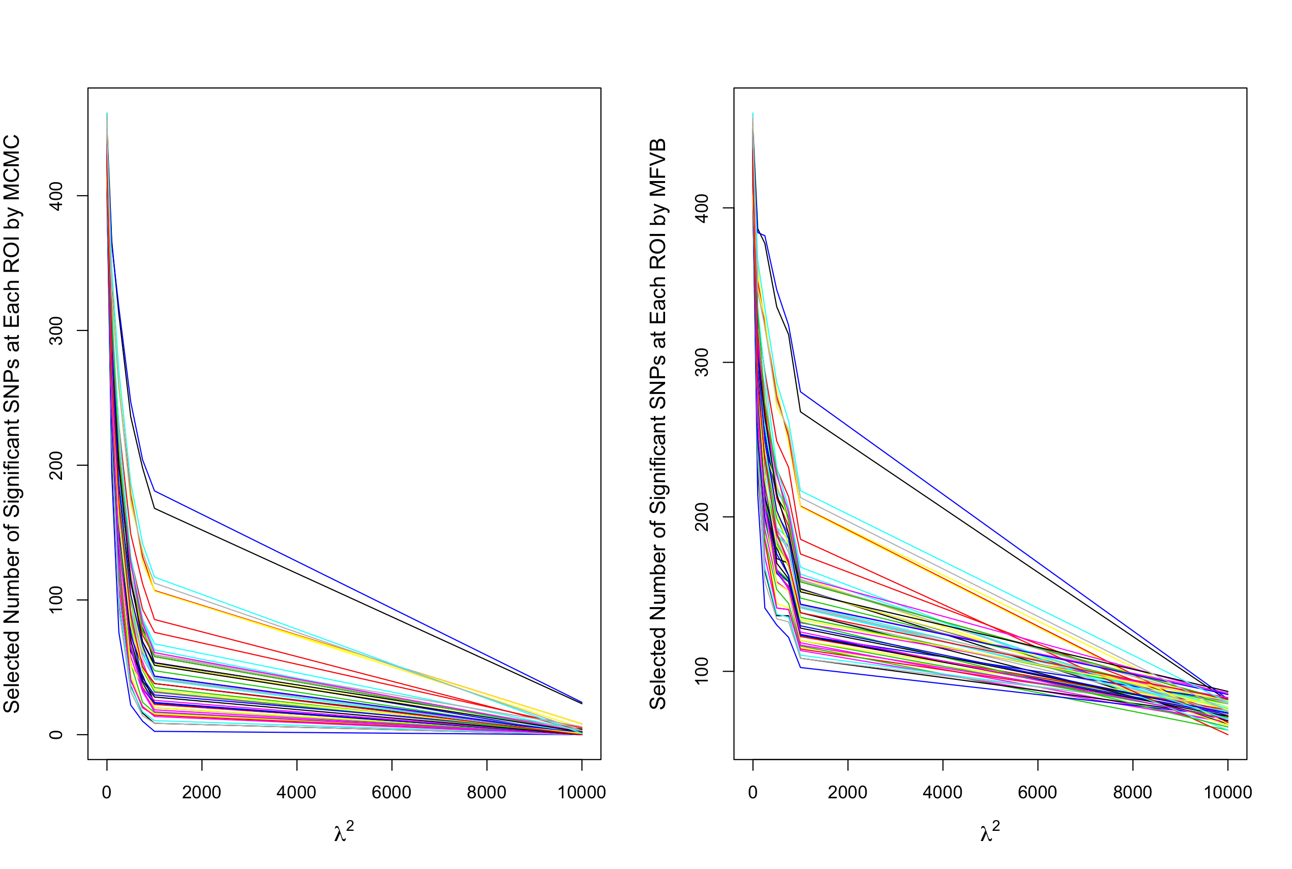
For the values of the tuning parameters $\rho=0.8$, $\lambda^{2}=10,000$, the average number of SNPs selected per ROI is 2, while more than half of the ROIs have no SNPs selected. In total, 75 SNPs across all 56 ROIs are selected and these are listed in Table 1 of the Supplementary Material along with the corresponding phenotypes that they are associated with. With the VB approximation, 150 SNPs are selected, and the set of SNP-ROI pairs selected by MCMC is a proper subset of the set selected by VB. In addition, the subset of SNPs and phenotypes also selected by the approach of Greenlaw et al. (2017) where the marginal posterior 95% credible interval is used for SNP selection are also highlighted in bold in Table 1 of the Supplementary Material.

Considering all three approaches, a consistent signal is found at the APOE gene, where all three methods select SNP rs405509 and the Bayesian FDR procedure selects this SNP for four phenotypes, namely, the middle temporal gyrus thickness on the right hemisphere, supramarginal gyrus thickness on the right hemisphere, mean thickness of the caudal midfrontal, rostral midfrontal, superior frontal, lateral orbitofrontal, and medial orbitofrontal gyri and frontal pole on the right hemisphere, and the mean thickness of the inferior temporal, middle temporal, and superior temporal gyri on the right hemisphere. We note that the selected associations for this SNP all correspond to ROIs in the right brain hemisphere. The associations between the genetic signal represented in our analysis by APOE SNP rs405509 with phenotypes on the right hemisphere of the brain may be of potential interest for further investigation.

The associated point estimates and 95% equal-tail credible intervals for all 56 phenotypes and APOE SNP rs405509 are presented in Table 3 of the Supplementary Material and a subset of these results for 26 phenotypes is presented in Table 2. Overall, there is broad agreement based on the overlap of the interval estimates, though, we also see a number of examples where the 95% interval estimate obtained from the spatial model includes the value 0 while the corresponding interval estimate for the non-spatial model does not include zero. The higher bias arising from VB in the simulation studies may also be apparent in the results presented in Table 2. The interval estimates arising from VB appear to be slightly more narrow than those obtained from MCMC, but not to a large degree, and this may also be reflected in the selection rates depicted in Figure 3 which are slightly higher. This is consistent with the coverage probabilities found in the first simulation study.

Another consistent signal is found at the ACE gene with SNP rs4311, which is found associated with 12 ROIs. We note that all but one of these ROIs is in the right hemisphere, and three of these ROIs (all of which are in the right hemisphere) are in common with the ROIs selected for this SNP by Greenlaw et al. (2017). In Figure 4 we indicate the SNPs chosen for each ROI, where the SNPs are grouped on the x-axis by gene and the ROIs are grouped in left/right pairs on the y-axis. The selected SNPs for each ROI are shown for tuning parameter values $\lambda^{2}=1000$ and $\lambda^{2}=10,000$. In both cases the value of the spatial tuning parameter for the CAR model is set at $\rho=0.8$ as suggested by Supplementary Material Figure 3.

Examining Figure 4, two ROIs stand out has having a relatively broad genetic signal that persists even as the tuning parameter increases from $\lambda^{2}=1000$ to $\lambda^{2}=10,000$. These are Left-Supramarg (thickness of the left supramarginal gyrus) and Left-SupTemporal (thickness of the left superior temporal gyrus). For the case where $\lambda^{2}=1000$, phenotype Left-Supramarg is associated with 188 SNPs (top panel of Figure 4) and this decreases to 24 SNPs (bottom panel of Figure 4) when $\lambda^{2}=10,000$. When $\lambda^{2}=1000$ phenotype Left-SupTemporal is associated with 188 SNPs and this decreases to 23 SNPs when $\lambda^{2}=10,000$. This is to be compared with the average number of SNPs selected over all ROIs when $\lambda^{2}=10,000$ which is just 2. The regularization paths for these two regions are shown in Supplementary Material Figure 4 where the SNPs having the most persistent signal across values of $\lambda^{2}$ are highlighted. These include SNP rs10868609 for the thickness of the left supramarginal gyrus and rs10501426 for the thickness of the left superior temporal gyrus.

We have developed a spatial multi-task regression model for relating genetic data to imaging phenotypes. The error structure for the imaging phenotype is based on a computationally convenient proper bivariate conditional autoregressive model, which allows us to account for bilateral correlation across brain hemispheres while also allowing us to account for within-hemisphere correlation using a graph structure. Examination of the data can assist in the determination of whether a model allowing for correlation is required. In our case it is clear that a model accounting for correlation is indeed required (see, e.g., Figure 1) for bilateral correlation. Empirical correlation between neighbouring regions can also be computed to determine if a simpler model should be considered. Examination of alternative spatial models and comparisons with respect to estimation, inference and robustness relative to that currently implemented under different settings will be part of future work.

Future developments may also incorporate the Bayesian false discovery probability proposed by Wakefield et al. (2007) which allows the user to account explicitly for the cost of false discoveries and the cost of false non-discovery. With regards to the two computational algorithms, we recommend that the approximate VB procedures be used to initialize the MCMC algorithm and also to obtain an initial insight into the data while the MCMC sampler runs. It appears that VB combined with Bayesian FDR tends to be more liberal in the selection of SNPs, and in our application the SNP-ROI pairs selected by MCMC + Bayesian FDR are a proper subset of that selected by VB + Bayesian FDR. Nevertheless, Figure 3 suggests that the approximation can be reasonable when good initializations are used.

Research is supported by funding from the Natural Sciences and Engineering Research Council of Canada and the Canadian Statistical Sciences Institute. F.S. Nathoo holds a Tier II Canada Research Chair in Biostatistics for Spatial and High-Dimensional Data. Research was enabled in part by support provided by WestGrid (www.westgrid.ca) and Compute Canada (www.computecanada.ca). Data collection and sharing for this project was funded by the Alzheimer’s Disease Neuroimaging Initiative (ADNI) (National Institutes of Health Grant U01 AG024904) and DOD ADNI (Department of Defense award number W81XWH-12-2-0012).

Recall that $\mbox{\boldmath$\omega$ \unboldmath}\!\!^{2}=(\omegao,\cdots,\omegad)$, $\tilde{W}_{i,j^{*}}=({W}_{i,j},W_{i,{j+1}})$, $i=1,...,d,~j=2j^{*}-1$,  $j^{*}=1,...,\frac{c}{2}$. based on the hierarchical prior setting, the joint posterior distribution can be expressed up to a normalizing constant as

$$\begin{split}p(\bm{W},\omegao,\cdots,\omegad,\bm{{\bm{\Sigma}}},|\bm{Y}){}&\propto{}p(\bm{Y}|\bm{W},\bm{{\bm{\Sigma}}})p(\bm{W}|\bm{{\bm{\Sigma}}},\mbox{\boldmath$\omega$ \unboldmath}\!\!^{2})p(\mbox{\boldmath$\omega$ \unboldmath}\!\!^{2})p(\bm{{\bm{\Sigma}}})\\ &\propto{}|(D_{A}-\rho A)^{-1}\otimes\bm{{\bm{\Sigma}}}|^{-\frac{n}{2}}\exp\Bigg\{-\frac{1}{2}\sum_{\ell=1}^{n}(\bm{y}_{\ell}-\bm{W}^{T}\bm{x}_{\ell})^{T}[(D_{A}-\rho A)^{-1}\otimes\bm{{\bm{\Sigma}}}]^{-1}\\ &(\bm{y}_{\ell}-\bm{W}^{T}\bm{x}_{\ell})\Bigg\}\\ &\times\prodid(\omega_{i}^{2})^{-\frac{c}{2}}|\bm{{\bm{\Sigma}}}|^{-\frac{c}{4}}\exp\{-\frac{1}{2}\sum_{j=1}^{\frac{c}{2}}\tilde{W}_{i,j}^{T}(\omega_{i}^{2}\bm{{\bm{\Sigma}}})^{-1}\tilde{W}_{i,j}\}\\ &\times\prodid\frac{{(\frac{\lambda^{2}}{2})^{\frac{c+1}{2}}}}{\Gamma(\frac{c+1}{2})}(\omega_{i}^{2})^{\frac{c}{2}-\frac{1}{2}}\exp\{-\frac{\lambda^{2}}{2}\omega_{i}^{2}\}\\ &\times\frac{|S|^{\frac{v}{2}}}{2^{v}\Gamma_{2}(\frac{v}{2})}|\bm{{\bm{\Sigma}}}|^{-\frac{v+3}{2}}\exp\left\{-\frac{1}{2}tr(S\bm{{\bm{\Sigma}}}^{-1})\right\}\\ \end{split}$$

The full conditional distribution of $\bm{W_{(i)}}$

For any matrix $A$, let $A_{(i)}$ be the $i_{th}$ row of $A$, $A_{i,j}$ be $i_{th}$ row and $j_{th}$ column of $A$ if $A$ is a matrix and $A_{(i)}$ be the $i_{th}$ element of $A$ if $A$ is a vector. And let $A_{(-i)}$ be the rest after removing $A_{(i)}$ from $A$. The full conditional distribution of $\bm{W_{(i)}},\;i=1,\dots,d$ is expressed as

$$(\bm{W}_{(i)})^{T}\big|\bm{Y},\bm{W}_{(-i)},\mbox{\boldmath$\omega$ \unboldmath}\!\!,\bm{{\bm{\Sigma}}}\sim MVN_{c}(\;\bvmui,\;\bm{{\bm{\Sigma}}}_{i}),$$

where

	$\displaystyle\bvmui$	$\displaystyle=\bm{{\bm{\Sigma}}}_{i}\Bigg(-\sumln(\bm{x}_{\ell(i)}\otimes I_{c})[(D_{A}-\rho A)\otimes\bm{{\bm{\Sigma}}}^{-1}](\bm{x}_{\ell(-i)}^{T}\otimes I_{c})(\bm{W}_{(-i)}^{T})$
		$\displaystyle+\sumln(\bm{x}_{\ell(i)}\otimes I_{c})[(D_{A}-\rho A)\otimes\bm{{\bm{\Sigma}}}^{-1}]\bm{y}_{\ell}\Bigg)$

$$\bm{{\bm{\Sigma}}}_{i}=\left(\bm{H}_{i}+\sumln(\bm{x}_{\ell(i)}\otimes I_{c})[(D_{A}-\rho A)\otimes\bm{{\bm{\Sigma}}}^{-1}](\bm{x}_{\ell(i)}^{T}\otimes I_{c})\right)^{-1}.$$

$$\bm{H}_{i}=\left[\left\{\frac{1}{\omega_{i}^{2}}\right\}\otimes I_{\frac{c}{2}}\otimes\bm{{\bm{\Sigma}}}^{-1}\right].$$

Since we already have the full conditional distribution, the coordinate-wise updates for mean field variational Bayes can be derived as:

	$\displaystyle q((\bm{W}_{(i)})^{T})$	$\displaystyle\propto exp\Big\{{\bf{E}}_{-i}(logP((\bm{W}_{(i)})^{T}|rest))\Big\}$
		$\displaystyle\propto exp\Big\{{\bf{E}}_{-i}\Big(-\frac{c}{2}log(2\pi)-\frac{1}{2}log(det|\bm{{\bm{\Sigma}}}_{i}|)-\frac{1}{2}((\bm{W}_{(i)})^{T}-\bvmui)^{T}\bm{{\bm{\Sigma}}}_{i}^{-1}((\bm{W}_{(i)})^{T}-\bvmui)\Big)\Big\}$
		$\displaystyle\propto exp\Big\{{\bf{E}}_{-i}\Big(-const-\frac{1}{2}(\bm{W}_{(i)})\bm{{\bm{\Sigma}}}_{i}^{-1}(\bm{W}_{(i)})^{T}+(\bm{W}_{(i)})\bm{{\bm{\Sigma}}}_{i}^{-1}\bvmui\Big)\Big\}$
		$\displaystyle\propto exp\Big\{const-\frac{1}{2}(\bm{W}_{(i)}){\bf{E}}_{-i}(\bm{{\bm{\Sigma}}}_{i}^{-1})(\bm{W}_{(i)})^{T}+(\bm{W}_{(i)}){\bf E}_{-i}\big(\bm{{\bm{\Sigma}}}_{i}^{-1}\bvmui\big)\Big\}$

REFERENCES

- [2] [] Bowman, F. D. (2005), “Spatio-temporal modeling of localized brain activity,” Biostatistics, 6(4), 558–575.
- [4] [] Bowman, F. D., Caffo, B., Bassett, S. S., and Kilts, C. (2008), “A Bayesian hierarchical framework for spatial modeling of fMRI data,” NeuroImage, 39(1), 146–156.
- [6] [] Corder, E. H., Saunders, A. M., Strittmatter, W. J., Schmechel, D. E., Gaskell, P. C., Small, G., Roses, A. D., Haines, J., and Pericak-Vance, M. A. (1993), “Gene dose of apolipoprotein E type 4 allele and the risk of Alzheimer’s disease in late onset families,” Science, 261(5123), 921–923.
- [8] [] Derado, G., Bowman, F. D., Zhang, L., and Initiative, A. D. N. (2013), “Predicting brain activity using a Bayesian spatial model,” Statistical methods in medical research, 22(4), 382–397.
- [10] [] Fischl, B. (2012), “FreeSurfer,” Neuroimage, 62(2), 774–781.
- [12] [] Gatz, M., Reynolds, C. A., Fratiglioni, L., Johansson, B., Mortimer, J. A., Berg, S., Fiske, A., and Pedersen, N. L. (2006), “Role of genes and environments for explaining Alzheimer disease,” Archives of general psychiatry, 63(2), 168–174.
- [14] [] Ge, T., Feng, J., Hibar, D. P., Thompson, P. M., and Nichols, T. E. (2012), “Increasing power for voxel-wise genome-wide association studies: the random field theory, least square kernel machines and fast permutation procedures,” Neuroimage, 63(2), 858–873.
- [16] [] Gelfand, A. E., and Banerjee, S. (2010), “Multivariate spatial process models,” Handbook of Spatial Statistics, pp. 495–515.
- [18] [] Gelfand, A. E., and Vounatsou, P. (2003), “Proper multivariate conditional autoregressive models for spatial data analysis,” Biostatistics, 4(1), 11–15.
- [20] [] Greenlaw, K., Szefer, E., Graham, J., Lesperance, M., Nathoo, F. S., and Initiative, A. D. N. (2017), “A Bayesian group sparse multi-task regression model for imaging genetics,” Bioinformatics, 33(16), 2513–2522.
- [22] [] Hibar, D. P., Stein, J. L., Kohannim, O., Jahanshad, N., Saykin, A. J., Shen, L., Kim, S., Pankratz, N., Foroud, T., Huentelman, M. J. et al. (2011), “Voxelwise gene-wide association study (vGeneWAS): multivariate gene-based association testing in 731 elderly subjects,” Neuroimage, 56(4), 1875–1891.
- [24] [] Hibar, D. P., Stein, J. L., Renteria, M. E., Arias-Vasquez, A., Desrivières, S., Jahanshad, N., Toro, R., Wittfeld, K., Abramovic, L., Andersson, M. et al. (2015), “Common genetic variants influence human subcortical brain structures,” Nature, 520(7546), 224.
- [26] [] Huang, C., Thompson, P., Wang, Y., Yu, Y., Zhang, J., Kong, D., Colen, R. R., Knickmeyer, R. C., Zhu, H., Initiative, A. D. N. et al. (2017), “FGWAS: Functional genome wide association analysis,” Neuroimage, 159, 107–121.
- [28] [] Huang, M., Nichols, T., Huang, C., Yu, Y., Lu, Z., Knickmeyer, R. C., Feng, Q., Zhu, H., Initiative, A. D. N. et al. (2015), “FVGWAS: Fast voxelwise genome wide association analysis of large-scale imaging genetic data,” Neuroimage, 118, 613–627.
- [30] [] Inkster, B., Nichols, T. E., Saemann, P. G., Auer, D. P., Holsboer, F., Muglia, P., and Matthews, P. M. (2010), “Pathway-based approaches to imaging genetics association studies: Wnt signaling, GSK3beta substrates and major depression,” Neuroimage, 53(3), 908–917.
- [32] [] Jin, X., Carlin, B. P., and Banerjee, S. (2005), “Generalized hierarchical multivariate CAR models for areal data,” Biometrics, 61(4), 950–961.
- [34] [] Kyung, M., Gill, J., Ghosh, M., Casella, G. et al. (2010), “Penalized regression, standard errors, and Bayesian lassos,” Bayesian Analysis, 5(2), 369–411.
- [36] [] Liu, J., and Calhoun, V. D. (2014), “A review of multivariate analyses in imaging genetics,” Frontiers in neuroinformatics, 8, 29.
- [38] [] Lu, Z.-H., Khondker, Z., Ibrahim, J. G., Wang, Y., Zhu, H., Initiative, A. D. N. et al. (2017), “Bayesian longitudinal low-rank regression models for imaging genetic data from longitudinal studies,” Neuroimage, 149, 305–322.
- [40] [] Lucotte, G., Loirat, F., and Hazout, S. (1997), “Pattern of gradient of apolipoprotein E allele* 4 frequencies in western Europe,” Human biology, pp. 253–262.
- [42] [] MacNab, Y. C. (2016), “Linear models of coregionalization for multivariate lattice data: a general framework for coregionalized multivariate CAR models,” Statistics in medicine, 35(21), 3827–3850.
- [44] [] Morris, J. S., Brown, P. J., Herrick, R. C., Baggerly, K. A., and Coombes, K. R. (2008), “Bayesian Analysis of Mass Spectrometry Proteomic Data Using Wavelet-Based Functional Mixed Models,” Biometrics, 64(2), 479–489.
- [46] [] Nathoo, F. S., Kong, L., and Zhu, H. (2018), “A Review of statistical methods in imaging genetics,” Canadian Journal of Statistics, p. DOI: 10.1002/cjs.11487.
- [48] [] Ormerod, J. T., and Wand, M. P. (2010), “Explaining variational approximations,” The American Statistician, 64(2), 140–153.
- [50] [] Park, T., and Casella, G. (2008), “The bayesian lasso,” Journal of the American Statistical Association, 103(482), 681–686.
- [52] [] Penny, W. D., Trujillo-Barreto, N. J., and Friston, K. J. (2005), “Bayesian fMRI time series analysis with spatial priors,” NeuroImage, 24(2), 350–362.
- [54] [] Purcell, S., Neale, B., Todd-Brown, K., Thomas, L., Ferreira, M. A., Bender, D., Maller, J., Sklar, P., De Bakker, P. I., Daly, M. J. et al. (2007), “PLINK: a tool set for whole-genome association and population-based linkage analyses,” The American Journal of Human Genetics, 81(3), 559–575.
- [56] [] Ren, Q., Banerjee, S., Finley, A. O., and Hodges, J. S. (2011), “Variational Bayesian methods for spatial data analysis,” Computational Statistics & Data Analysis, 55(12), 3197–3217.
- [58] [] Scott, S. L., Blocker, A. W., Bonassi, F. V., Chipman, H. A., George, E. I., and McCulloch, R. E. (2016), “Bayes and big data: The consensus Monte Carlo algorithm,” International Journal of Management Science and Engineering Management, 11(2), 78–88.
- [60] [] Shen, X., Papademetris, X., and Constable, R. T. (2010), “Graph-theory based parcellation of functional subunits in the brain from resting-state fMRI data,” Neuroimage, 50(3), 1027–1035.
- [62] [] Silver, M., Montana, G., Nichols, T. E., Initiative, A. D. N. et al. (2011), “False positives in neuroimaging genetics using voxel-based morphometry data,” Neuroimage, 54(2), 992–1000.
- [64] [] Stein, J. L., Hua, X., Lee, S., Ho, A. J., Leow, A. D., Toga, A. W., Saykin, A. J., Shen, L., Foroud, T., Pankratz, N. et al. (2010), “Voxelwise genome-wide association study (vGWAS),” Neuroimage, 53(3), 1160–1174.
- [66] [] Stein, J. L., Medland, S. E., Vasquez, A. A., Hibar, D. P., Senstad, R. E., Winkler, A. M., Toro, R., Appel, K., Bartecek, R., Bergmann, Ø. et al. (2012), “Identification of common variants associated with human hippocampal and intracranial volumes,” Nature genetics, 44(5), 552.
- [68] [] Stingo, F. C., Guindani, M., Vannucci, M., and Calhoun, V. D. (2013), “An integrative Bayesian modeling approach to imaging genetics,” Journal of the American Statistical Association, 108(503), 876–891.
- [70] [] Szefer, E., Lu, D., Nathoo, F., Beg, M. F., Graham, J. et al. (2017), “Multivariate association between single-nucleotide polymorphisms in Alzgene linkage regions and structural changes in the brain: discovery, refinement and validation,” Statistical applications in genetics and molecular biology, 16(5-6), 367–386.
- [72] [] Teng, M., Johnson, T. D., and Nathoo, F. S. (2018a), “Time series analysis of fMRI data: Spatial modelling and Bayesian computation,” Statistics in medicine, .
- [74] [] Teng, M., Nathoo, F. S., and Johnson, T. D. (2018b), “Bayesian analysis of functional magnetic resonance imaging data with spatially varying auto-regressive orders,” Journal of the Royal Statistical Society: Series C (Applied Statistics), .
- [76] [] Thompson, P. M., Ge, T., Glahn, D. C., Jahanshad, N., and Nichols, T. E. (2013), “Genetics of the connectome,” Neuroimage, 80, 475–488.
- [78] [] Vehtari, A., Gelman, A., and Gabry, J. (2017), “Practical Bayesian model evaluation using leave-one-out cross-validation and WAIC,” Statistics and Computing, 27(5), 1413–1432.
- [80] [] Vounou, M., Janousova, E., Wolz, R., Stein, J. L., Thompson, P. M., Rueckert, D., Montana, G., Initiative, A. D. N. et al. (2012), “Sparse reduced-rank regression detects genetic associations with voxel-wise longitudinal phenotypes in Alzheimer’s disease,” Neuroimage, 60(1), 700–716.
- [82] [] Vounou, M., Nichols, T. E., Montana, G., Initiative, A. D. N. et al. (2010), “Discovering genetic associations with high-dimensional neuroimaging phenotypes: A sparse reduced-rank regression approach,” Neuroimage, 53(3), 1147–1159.
- [84] [] Wakefield, J. (2007), “A Bayesian measure of the probability of false discovery in genetic epidemiology studies,” The American Journal of Human Genetics, 81(2), 208–227.
- [86] [] Wang, H., Nie, F., Huang, H., Risacher, S. L., Saykin, A. J., Shen, L., and Initiative, A. D. N. (2012), “Identifying disease sensitive and quantitative trait-relevant biomarkers from multidimensional heterogeneous imaging genetics data via sparse multimodal multitask learning,” Bioinformatics, 28(12), 127–136.
- [88] [] Zhu, H., Khondker, Z., Lu, Z., and Ibrahim, J. G. (2014), “Bayesian generalized low rank regression models for neuroimaging phenotypes and genetic markers,” Journal of the American Statistical Association, 109(507), 977–990.
- [89]
Supplementary Material for the ’A Bayesian Spatial Model for Imaging Genetics’
Web Appendix A: Selected SNPs and the Corresponding Regions of Interest for the ADNI-1 Application