Solution of the Metropolis dynamics on a complete graph with application to the Markov chain Mpemba effect
Abstract
We find analytically the complete set of eigenvalues and eigenvectors associated with Metropolis dynamics on a complete graph. As an application, we use this information to study a counter-intuitive relaxation phenomenon, called the Mpemba effect. This effect describes situations when upon performing a thermal quench, a system prepared in equilibrium at high temperatures relaxes faster to the bath temperature than a system prepared at a temperature closer to that of the bath. We show that Metropolis dynamics on a complete graph does not support weak nor strong Mpemba effect, however, when the graph is not complete, the effect is possible.
Keywords:
Relaxation toward equilibrium, Monte Carlo, Mpemba effect, Quench dynamics, Markov jump processes, MetropolisI Introduction
Monte Carlo algorithms are widely used in diverse fields of science, Sokal 1997; Krauth 2006. In particular, they are often the tool of choice when estimating multidimensional integrals present in statistical physics and quantum field theory. Typically in physical systems, describing the real world, the phase space is exponentially large. Monte Carlo algorithms are especially useful for sampling equilibrium properties, and estimating equilibrium observables, where direct sampling is unfeasible due to an exponentially large phase space. Their convergence properties are widely studied, see, e.g. Levin et al. 2009.
In a typical implementation for a system with states, one specifies the probability distribution where is the probability for the system to be in state at time . The evolution of the system is assumed to depend only on the present, i.e. it is Markovian, and it obeys a Master equation
| (1) |
where the off-diagonal matrix element is the rate (probability per unit time) to jump from state to . The diagonal elements of the rate matrix are ”escape rates”
| (2) |
set so that the sum over any column of gives zero. This constraint ensures the conservation of probability. For a general treatment, see e.g. Sokal 1997; Levin et al. 2009. We will assume that under the Markov evolution, the system converges to a steady state, . The global balance condition guarantees that total flux from any of state of the systems is equal to the total influx to that state, or
| (3) |
Typically, such a non-local condition is hard to implement in practice, except for select cases, see, e.g. Turitsyn et al. 2011; Vucelja 2016. Detailed balance is a special case of Eq. (3)
| (4) |
Despite often slow relaxations to a steady state Turitsyn et al. 2011; Vucelja 2016, Markov jump processes obeying detailed balance, are preferred, as detailed balance is an easily implementable, local condition. In particular, one of the most popular Monte Carlo jump process dynamics, that obeys detail balance is the Metropolis dynamics Metropolis et al. 1953. Metropolis dynamics is described by the following transition acceptance rate from state to state :
| (5) |
Note that it is always possible to view the steady state as a thermal equilibrium, by writing , i.e. the Bolzmann distribution at some temperature and would correspond to energies. A particularly simple choice is , which sets and .
In this paper, we solve for the eigensystem of Metropolis dynamics for a complete graph, as described in the next section. We then use the slowest relaxing eigenvector to explore the possibility of a Mpemba effect (defined below) in such a system.
II Metropolis dynamics on a complete graph
When only transitions between specific pairs of states appear in the rate matrix , we say that the Metropolis dynamics takes place on a graph corresponding to the adjacency matrix , where if is allowed, if is not allowed, and set =0. The rule (5), without further restriction on which pairs of states and admit transitions, describes dynamics on a complete graph. Otherwise, if only transitions between certain pairs of states are allowed directly in , the graph is not complete. For example for a spin system, one often studies the Glauber dynamics, where only states differing by a single spin state are connected Glauber 1963.
Due to the appearance of the in the form of the transition matrix (5), the matrix is non-analytic as a function of the energy levels. Despite this non-analyticity, we find, somewhat surprisingly, that the entire spectral decomposition of is given in a simple form. The results are expressed in the following theorem below.
We will use the standard basis vectors , where is an dimensional vector, with is in the th place.
Theorem: Let an ordering of the steady state probabilities be given by a permutation , s.t. , or, equivalently, the energies corresponding to the steady state distribution are ordered as
| (6) |
Let the permutation matrix realizing the permutation be , s.t. The first eigenvalue and its associated eigenvector of the Metropolis are
| (7) |
The rest of the eigenvalues, ordered by absolute value, are given by , where
| (8) | ||||
| (9) |
are the eigenvectors of the system in the basis where the are ordered by magnitude. Here
| (10) |
Proof: Below for convenience we chose to work with the Boltzmann form of the instead of directly with . First, we note that for any ordering of the energies, we can use the transformation to first work in a basis where the energies are ordered according to their magnitude. It will therefore be enough to prove the relation under the assumption that the energy levels are ordered as at the outset. In the end we just return to the original ordering by applying to the resulting eigenvectors. We will now do induction on the number of energy levels. Our induction assumption is that for ,
| (11) |
are the eigenstates of with corresponding eigenvalues . In addition we have the vector
| (12) |
as a zero eigenvector by construction of the Metropolis matrices. We first check our initial assumptions on a Metropolis system, with energies . The matrix is:
| (13) |
This system has the eigenvectors and eigenvalues:
| (14) | ||||
| (15) |
These eigenvalues fit the desired form.
We will assume that the form is correct for levels , and then consider adding another energy level to the complete graph. With the energy ordering chosen, the matrix has the form:
Now we add a new energy . We write the new matrix as:
| (18) |
where the lower right block in the first term is simply . Below we will be using the natural basis elements labeled as: . We will define:
| (19) |
and
| (20) |
With these definitions
| (21) |
To compare with our induction assumptions, we will label the eigenvectors of the new state system , for , and we will use the correspondences for the energies and for the vectors. In addition, we now have: . Note that the above definition implies the relation: .
We now proceed with the induction, separating into the following cases:
(i) . By the construction of Metropolis, we already know that
| (22) |
is the eigenvector with eigenvalue zero.
(ii) . Let us check that indeed are the desired eigenstates. First, notice that:
| (23) |
We now explicitly apply :
| (24) |
where we have used the induction hypothesis:
| (25) |
| (26) |
and that for
| (27) |
Finally, using we have:
| (28) |
showing that is of the desired form.
It is left to check the form for . We write:
| (29) |
Applying explicitly, we have:
| (30) |
Finally we note that:
| (31) |
giving:
| (32) |
which is consistent with: at . This concludes our proof.
In the next section, we define an interesting counter-intuitive relaxation behavior called the Mpemba effect. Afterward, we apply our results for the Metropolis dynamics, to study the existence of the Mpemba effect for Metropolis dynamics on a complete graph.
III Relaxation with Metropolis dynamics and the Mpemba effect
The Mpemba effect is a surprising relaxation phenomenon known already since Aristotle times Aristotle 1962. The effect is encountered when a hot liquid relaxes faster to equilibrium than a cold one when they are coupled with a cold bath Mpemba and Osborne 1969. The effect has been observed several systems, including clathrate hydrates Ahn et al. 2016, polymers Hu et al. 2018, magnetic alloys Chaddah et al. 2010, carbon nanotube resonators Greaney et al. 2011, granular gases Lasanta et al. 2017 as well, as in a dilute atomic gas Keller et al. 2018.
A phenomenological description of such behavior for Markovian dynamics was recently given in Lu and Raz 2017; Klich et al. 2017. This approach allows for the investigation of Mpemba like behavior in many different systems as Markovian dynamics is an excellent description of many processes in physics and chemistry (see, e.g. van Kampen N. G. 2001).
To describe the effect, we assume the relaxation is governed by a master equation with a transition rate matrix as described above. In the Mpemba effect case, we take the initial condition for Eq. (1) the thermal equilibrium at some temperature , where is the bath temperature:
| (33) |
During the relaxation process, the distribution — i.e. the solution of Eq. (1) – is
| (34) |
where the rate matrix has (right) eigenvectors and eigenvalues . The largest eigenvalue of , , is associated with the stationary (equilibrium) distribution , whereas all the other eigenvalues have negative real parts, and they correspond to the relaxation rates of the system. The equilibration timescale is typically characterized by 11 1 For detailed balance matrices , the eigenvalues are all real..
IV Existence of Mpemba effects with Metropolis dynamics
We are now in position to utilize our established result for the second eigenvector of Metropolis dynamics on a complete graph. The presence of a Mpemba effect in a relaxation process like Eq. (1) can be characterized as follows Lu and Raz 2017. Assume that ( are actually real for the Metropolis system), then at long times the probability distribution (34) is approximated as
| (35) |
We say that an Mpemba effect exists in this system if there are three temperatures , such that
| (36) |
In other words at long times, the system prepared at is closer to the bath equilibrium distribution than a system prepared at , although is closer to the bath temperature . In Klich et al. 2017 a stronger variant of the effect was proposed, where at some temperature , we have , signaling a jump in relaxation times (). An analogues ”inverse” Mpemba effect is also possible with . We summarize all the above cases as in the following definition:
We say that a system has a strong Mpemba effect if there exists a temperature for which , and a weak Mpemba effect if is a non-monotonic function on either or (or on both).
In the next section we show that in our system of Metropolis on a complete graph, both the weak and strong Mpemba effects are absent. Finally, we show a example where these effects are possible for Metropolis on a graph which is incomplete.
IV.1 Absence of Mpemba effect with Metropolis on a complete graph
We will use the following expression for , derived in Lu and Raz 2017,
| (37) |
where is a diagonal matrix with elements , and a constant that depends only on the bath and choice of normalization for the eigenvector . Explicitly using our result for , we have:
| (38) |
Finally we note that if we assume the spectrum is not completely degenerate, then:
| (39) |
since for at least one by the assumption that the spectrum is not completely degenerate. This implies that can only vanish at a single point, that is at . In fact, we see that is a monotonic function, ruling out both strong and weak Mpemba effects.
IV.2 Mpemba effect with Metropolis on a graph with a single edge removed
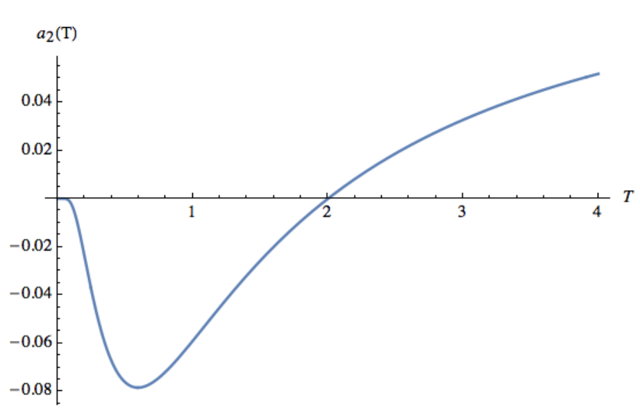
We now show in a simple example that an Mpemba effect can happen when some of the are set to zero. Let us consider the following transition matrix:
This matrix blocks direct transitions. The matrix has eigenvalues , with the second eigenvector given simply by:
| (44) |
Computing using (37) we have:
| (45) |
Notice that , as should be the case, however, in addition, we see that . Thus between and (the limit of low temperatures), cannot be monotonic, implying an indirect Mpemba effect, as can be seen in the figure 1.
V Discussion
In this paper, we have shown how the eigenvectors and eigenvalues of the Metropolis dynamics on a complete graph are analytically given when no transitions are blocked. The simplicity of the result is somewhat surprising since the matrix formally depends non-analytically on the energies at energy crossings. As an application we have shown that the Markovian Mpemba effect is not present in this system. The result can be anticipated, as it means that the flow to lower temperatures cannot get ”stuck” at an intermediate temperature. On sparser graphs though, the Mpemba effect can arise. Indeed, we give an example of the effect on a simple 3 level example, where one direct transition in the Metropolis dynamics has been set to zero. For larger systems, one can look at the Metropolis simulations of spin-glass in Janus collaboration et al. 2018, which show the Mpemba effect.
It is important to note, though, that in most practical applications, i.e., as a numerical tool, the Metropolis is mostly used on systems with sparse adjacency graphs. On a general graph, an exact solution is not likely. However, the present approach allows for a perturbative treatment when edges of the adjacency graph are removed.
Acknowledgement: The authors thanks Oren Raz for insightful remarks. The work of IK was supported by the NSF grant DMR-1508245. This research was supported in part by the National Science Foundation under Grant No. NSF PHY-1748958.
References
- Sokal (1997) A. Sokal, in Functional Integration, edited by C. DeWitt-Morette, P. Cartier, and A. Folacci (Springer US, New York, NY, USA, 1997), vol. 361 of NATO ASI Series, pp. 131–192.
- Krauth (2006) W. Krauth, Statistical Mechanics: Algorithms and Computations (Oxford University Press, Oxford, 2006).
- Levin et al. (2009) D. A. Levin, Y. Peres, and E. L. Wilmer, Markov Chains and Mixing Times (American Mathematical Society, Providence, RI, USA, 2009).
- Turitsyn et al. (2011) K. Turitsyn, M. Chertkov, and M. Vucelja, Physica D Nonlinear Phenomena 240, 410 (2011).
- Vucelja (2016) M. Vucelja, American Journal of Physics 84, 958 (2016).
- Metropolis et al. (1953) N. Metropolis, A. Rosenbluth, M. Rosenbluth, A. Teller, and E. Teller, J. of Chem. Phys. 21, 1087 (1953).
- Glauber (1963) R. J. Glauber, J. Math. Phys. 4, 294 (1963).
- Aristotle (1962) Aristotle, Meteorologica (Harvard U. P., 1962), translated by H.D.P. Lee, Book I, Chap. XII.
- Mpemba and Osborne (1969) E. B. Mpemba and D. G. Osborne, Physics Education 4, 172 (1969), URL http://stacks.iop.org/0031-9120/4/i=3/a=312.
- Ahn et al. (2016) Y.-H. Ahn, H. Kang, D.-Y. Koh, and H. Lee, Korean Journal of Chemical Engineering pp. 1–5 (2016).
- Hu et al. (2018) C. Hu, J. Li, S. Huang, H. Li, C. Luo, J. Chen, S. Jiang, and L. An, Crystal Growth & Design 18, 5757 (2018).
- Chaddah et al. (2010) P. Chaddah, S. Dash, K. Kumar, and A. Banerjee, arXiv preprint arXiv:1011.3598 (2010).
- Greaney et al. (2011) P. A. Greaney, G. Lani, G. Cicero, and J. C. Grossman, Metallurgical and Materials Transactions A 42, 3907 (2011).
- Lasanta et al. (2017) A. Lasanta, F. Vega Reyes, A. Prados, and A. Santos, Phys. Rev. Lett. 119, 148001 (2017), URL https://link.aps.org/doi/10.1103/PhysRevLett.119.148001.
- Keller et al. (2018) T. Keller, V. Torggler, S. B. Jäger, S. Schütz, H. Ritsch, and G. Morigi, New Journal of Physics 20, 025004 (2018).
- Lu and Raz (2017) Z. Lu and O. Raz, Proceedings of the National Academy of Sciences 114, 5083 (2017).
- Klich et al. (2017) I. Klich, O. Raz, O. Hirschberg, and M. Vucelja, ArXiv e-prints (2017).
- van Kampen N. G. (2001) van Kampen N. G., Stochastic processes in physics and chemistry (Elsevier, 2001).
- Janus collaboration et al. (2018) Janus collaboration, M. Baity-Jesi, E. Calore, A. Cruz, L. A. Fernandez, J. M. Gil-Narvion, A. Gordillo-Guerrero, D. Iñiguez, A. Lasanta, A. Maiorano, et al., ArXiv e-prints (2018).