Robust random search with scale-free stochastic resetting
Abstract
A new model of search based on stochastic resetting is introduced, wherein rate of resets depends explicitly on time elapsed since the beginning of the process. It is shown that rate inversely proportional to time leads to paradoxical diffusion which mixes self-similarity and linear growth of the mean square displacement with non-locality and non-Gaussian propagator. It is argued that such resetting protocol offers a general and efficient search-boosting method that does not need to be optimized with respect to the scale of the underlying search problem (e.g., distance to the goal) and is not very sensitive to other search parameters. Both subdiffusive and superdiffusive regimes of the mean squared displacement scaling are demonstrated with more general rate functions.
I Introduction
Any search is intrinsically governed by randomness: the need to perform it underscores the ignorance of the searching agent and its inability to predict the outcome. In particular, the agent may not know in advance how much time, on average, it will take to find a target and how much variability in search time is expected due the randomness. How can the efficiency of a search strategy be boosted without acquiring such information beforehand? It may happen that the longer the search lasts, the more unfavorable random instance the agent is experiencing, and thus the longer the expected remaining time to find the target. It is then true that restarting the process anew may be beneficial, as it lowers the expected completion time. It has been shown that this is indeed the case if the coefficient of variation of completion times is larger than Reuveni2016. This conditions holds if the completion times of a search process are drawn from the hyperexponential or power-law distributions. Such situation arises, for instance, in the one-dimensional, unbiased Brownian motion with a single target. The possibility of arbitrarily long excursions far from the target manifests itself in large fluctuations and the associated power-law distribution of the first passage times.
In the engineering community such mechanism was studied in the context of computer software systems huang1995software; dohi2001estimating; van2006analysis; okamura2016analysis and non-convex optimization methods fukunaga1998restart; jansen2002analysis; luersen2004globalized; loshchilov2016sgdr. More recently, Evans and Majumdar introduced a model with time-homogeneous stochastic resetting (i.e., with exponentially distributed waiting times between the resets) in tandem with diffusion majumdar2011resetting. They showed that one-dimensional majumdar2011resetting and multidimensional evans2014diffusion diffusion with resets exhibit finite mean first passage times (MFPTs) which can be optimized with respect to resetting rate . Moreover, resets lead to non-equilibrium steady-states with a combination of local and non-local currents majumdar2011resetting; mendez2016characterization; eule2016non. The simplicity and nontrivial behavior of these systems has sparked the interest of the physics community, with a considerable amount of research focusing on modifying the model to include nontrivial boundary conditions christou2015diffusion; chatterjee2018diffusion; pal2018first, external potentials pal2015diffusion, anomalous transport kusmierz2014first; kusmierz2015optimal; mendez2016characterization; shkilev2017continuous; Montero2017; bodrova2018scaled; bodrova2018non; kusmierz2019subdiffusive, drift Montero2017; ray2018p, delays following the resets Reuveni2016; evans2018effects; maso2019stochastic; pal2019home, and non-exponential distributions of waiting times between resets nagar2016diffusion; eule2016non; pal2016diffusion. Resets were also studied in the context of stochastic energetics fuchs2016stochastic, enzymatic reactions rotbart2015michaelis, fluctuating interfaces gupta2014fluctuating, and power-law distributions in non-equilibrium systems manrubia1999stochastic.
Non-exponential waiting times between the resets can be generated by time-dependent resetting rates nagar2016diffusion; pal2016diffusion. In models introduced in these previous works, rate depends on the time elapsed since the last reset. Here we introduce a new model with resetting rate that depends on the time elapsed since the start of the process. Such non-stationary resetting protocol, while preserving the Markovian character of the dynamics, introduces time-inhomogeneity. As we will show, this dramatically affects the behavior of the process. If decays with time, the process does not converge to any steady state, with the mean square displacement (MSD) growing indefinitely. Moreover, that is inversely proportional to time provides an efficient and robust mechanism to boost the time efficiency of a search. It has previously been shown that deterministic resetting is the optimal way of minimizing search time via resets pal2016first. However, similarly to stochastic resetting with a constant rate, such resetting has to be optimized assuming full knowledge of details of a given search problem. In contrast, the resetting mechanism we propose does not have to be adapted to the time scale of the search problem.
II Diffusion with time-dependent resetting
We start from one-dimensional diffusion as the underlying search process, which will help build the intuition. Later we present a more general framework. Since the process of diffusion with memoryless resetting is Markovian, it is fully characterized by the initial position distribution and the propagator , which denotes the probability density function of at time of a particle that at time was at . The particle diffuses till a resetting event that brings it instantaneously back to the resetting position (equal to the position of the particle at time ) 11 1 We are assuming that the initial position corresponds to the resetting position. However, due to the singular behavior of the function at , the choice of the initial position is inconsequential: If it does not match the resetting position, the probability mass is transferred to the resetting position in an infinitesimal time. . The particle then continues to diffuse until the next reset. The corresponding propagator solves the following partial differential equation
| (1) |
where denotes the partial derivative with respect to and is the diffusion coefficient. Such process has been analyzed extensively in the case of a constant rate , with the corresponding resets described by the homogeneous Poisson point process. It has been shown majumdar2011resetting that this process, in the absence of targets, attains a non-equilibrium steady state. If a single target, represented by an absorbing boundary, is placed at the origin, there exists an optimal rate at which the MFPT is minimized.
II.1 Scale-free resetting
In this work we mainly focus our attention on the special case of
| (2) |
The only parameter is dimensionless—this form of resetting does not introduce any time scale. For this reason, we refer to (2) as a scale-free resetting. Resets described by (2) are generated by the inhomogeneous Poisson point process with an average intensity (expected number of events) within a time period given by
| (3) |
Note that our choice of features a singularity at , which translates into diverging intensity with . Any practical applications of scale-free resetting have to introduce a short-term cut-off to avoid resetting with infinite frequency. However, all our theoretical predictions without an explicit account of the cut-off are still valid at times much longer than the cut-off.
As evident from (1), the process (1) with (2) preserves the self-similarity of the pure Brownian motion, i.e., the re-scaling and does not change any observables (see Fig. 1).

We can therefore expect that the mean square displacement (MSD) scales linearly with time. Indeed, straightforward calculations (multiply (1) by , integrate over and solve the resulting ordinary differential equation) lead to
| (4) |
Although the self-similarity and associated linear time-dependence of the MSD bear a strong resemblance to free diffusion, resets vastly modify other statistics. For instance, the Fourier transform of the propagator reads
| (5) |
This propagator is clearly non-Gaussian and has a cusp at . It takes a particularly simple form for
| (6) |
Similar non-Gaussian displacement distributions with a cusp, accompanied by a linear time dependence of the MSD have been observed in several systems of diffusing colloidal particles wang2009anomalous; wang2012brownian. Such systems have recently attracted considerable attention among theoreticians, who since then have developed multiple models with fluctuating diffusivity hapca2008anomalous; wang2009anomalous; chubynsky2014diffusing; chechkin2017brownian; sposini2018random. Scale-free resetting provides an alternative mechanism behind such behavior.
II.2 Generalizations of the resetting rate function
In addition to the presented applications to search problems, a generalization of the proposed resetting mechanism can be applied to model anomalous transport phenomena. The MSD of (1) with is given by the formula
| (7) |
which for exhibits a smooth transition between diffusive behavior with the MSD for and subdiffusive behavior with the MSD for , where is the time scale introduced by the power-law resetting. In the opposite case of the long-term behavior is diffusive, whereas at short times an apparent superdiffusivity with the MSD is observed. By assuming one can also model an ultra-slow diffusion with the MSD , a behavior previously uncovered in the strongly non-Markovian random walks with preferential relocations to places visited in the past boyer2014random.
One could involve heavy-tails jump distributions leading to a competition between superdiffusivity of the Lévy flights and subdiffusive tendency from resets, similar to the competition observed in the continuous-time random walk scheme montroll1965random; metzler2000random; magdziarz2007competition. Many different variants of a combination of anomalous transport with constant-rate stochastic resetting were previously studied kusmierz2014first; kusmierz2015optimal; mendez2016characterization; shkilev2017continuous; Montero2017; kusmierz2019subdiffusive and were shown to exhibit non-trivial features, including first and second order transitions of the optimal search kusmierz2014first; kusmierz2015optimal; campos2015phase; Montero2017 and a non-monotonic behavior of the MSD kusmierz2019subdiffusive. For this reason, we expect that a combination of scale-free resets with independent constant-rate resets may lead to thought-provoking phenomena.
III Completion times
In the previous section we have shown how time-dependent resetting affects the time evolution and shape of the displacement distribution. Another striking consequence of scale-free resetting can be observed in the statistics of the first passage times. As we show in the following, in contrast to free diffusion on infinite line, diffusion with scale-free resetting can find a target in a finite MFPT. Moreover, due to the self-similarity, we can expect that the MFPT is proportional to , where denotes the initial position with respect to the target.
This observation prompted us to explore more general scenarios of search under scale-free resetting beyond diffusion on intinite line. Since the following calculations apply to general search times that may not be generated as the first passage times of some stochastic process, we hereafter use the term completion times. We show that scale-free resetting is robust, i.e. the optimal form of the scale-free resetting (as prescribed by the parameter ) does not depend on the time scale. Thus, the protocol can be optimized in a parsimonious manner, without knowing how much time on average the underlying search takes.
III.1 General analysis
Instead of assuming that the underlying search process is described by a simple, one-dimensional diffusion, we first consider any random search process. Let a non-negative random variable be the completion times of the original process without resetting. Similarly, let denote the completion times of the same process modified by introducing scale-free resets of the form (2). Our goal is to calculate statistics of given known statistics of . In particular, we will be interested in the mean completion time (MCT), denoted as . For any absolute-time-dependent rate function , one can link the survival probability of the model with resets with the survival probability of the underlying reset-free process by means of the following renewal equation 22 2 Note that multiple different renewal approaches to processes with resetting have been proposed gupta2014fluctuating; Reuveni2016; pal2016first; chechkin2018random. Our approach is closely related to a discrete-time counterpart applied in kusmierz2014first.
| (8) |
where
| (9) |
is the probability of no resets in the interval of time . Eq. (8) splits the survival probability into two cases: either there are no resets until time , which happens with probability , or there are resets in this time period with the last reset at time . The integral appears here because can be anywhere between and . In the case of scale-free resetting (2), the no-reset probability is given by
| (10) |
Combining the general expression (8) with (10) and (2) we arrive at the equation
| (11) |
In order to solve Eq. (11) we introduce an auxillary function
| (12) |
which solves a simpler integral equation
| (13) |
By denoting as the Laplace transform of , the corresponding Laplace-transformed equation reads
| (14) |
In the following we will assume that the probability of finding the target in no-time is equal to zero. In this case the corresponding survival probability can be written in the form redner2001guide
| (15) |
where is the probability density function of the completion time of the process without resetting, and . We can easily solve the differential equation (14) leading to
| (16) |
where is a constant yet to be determined.
We now show how to recover from . We employ the identity
| (17) |
which holds for 33 3 The integral operator in (17) and (18) corresponds to the Riemann-Liouville fractional integral. Similarly, the integral in (19) can be expressed by means of the Caputo fractional derivative. . From (17) we deduce that
| (18) |
We can apply (18) in (12) by replacing with and noticing that 44 4 We could have also applied (18) directly with . The resulting equation is simpler, but holds only for . , which leads to
| (19) |
In the last step we plug (16) into (19). The initial condition
| (20) |
allows us to calculate . The final result reads
| (21) |
Eq. (21) allows us to calculate any statistics of the completion times, at least in principle. In particular, the MCT is simply given by , i.e.
| (22) |
III.2 Special cases
Here we present two special cases of the search process , which illustrates basic features of the scale-free resetting.
III.2.1 1D diffusion with a single trap
In the first example we consider one-dimensional diffusion (1) with a single target (trap). The probability density function of the completion times (here corresponding to the first passage times) for (no resets) is well-known and in the Laplace space reads redner2001guide
| (23) |
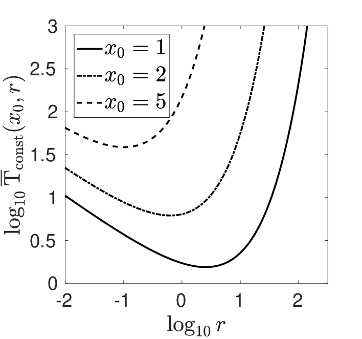
where . Importantly, for large and thus the MCT is infinite. Plugging (23) into the general expression for the MCT (22) leads to a rather complicated integral, which can nevertheless be easily integrated numerically. Numerical simulations confirm our theoretical prediction (cf. Fig. 2) and show that the MCT attains its minimum value of at . Moreover, as expected from the dimensionality analysis, the MCT scales quadratically with the initial distance to the target.
We can learn a lot about the distribution of by directly analyzing the auxiliary function (16), which in the case of diffusion takes the form
| (24) |
where
| (25) |
is a version of the exponential integral. For it can be expressed as
| (26) |
where stands for the Euler-Mascheroni constant. Thus the solution (24) has the following representation
| (27) |
By letting in (27) we arrive at a simple formula for the -th (fractional) moment
| (28) |
For we obtain a simple expression for the MCT
| (29) |
As expected, the MCT scales quadratically with the distance to the target. Small expansion of (27) shows that for large , which together with (12) implies that the tail of the survival probability behaves like
| (30) |
Therefore, the fractional moments are finite if and only if . In particular, the MCT is finite for , see Fig. 2.

III.2.2 Random search with failure
As we show in Section III.3, the optimal choice of does not depend on the search-problem time scale. However, this choice may be sensitive to other features of . In the second example we explore the resilience of the scale-free resetting to search failures. Let the search problem be described by the density
| (31) |
where is the probability of a successful search. The trivial case corresponds to deterministic completion time, whereas for the density is unnormalized as there is non-zero probability that the search ends with a failure, i.e. the completion time is infinite. We plug
| (32) |
into (16) and arrive at
| (33) |
and thus via the expansion (26)
| (34) |
for and large . We conclude that the MCT is finite if and only if or , see Fig. 3. Moreover, the MCT is again proportional to time scale :
| (35) |
This example illustrates the fact that, while robust to the time scale, scale-free resetting may be sensitive to other features of the search problem. In particular, the higher the probability of the search failure, the larger resetting intensity is necessary to assure a finite value of the MCT. We discuss this issue in more detail in Section III.4.3.
III.3 Linear scale-dependence
We have seen that in two simple special cases the MCT is proportional to the time scale of the underlying search problem. Here we show that this is always the case and that this observation generalizes to higher moments. Given the completion time of a process without resets , we define a rescaled completion time as . As in Section III.2.2, the parameter denotes the time-scale of the search problem, and may be related to its different features, e.g. in the case of diffusion is proportional to . The corresponding probability density functions are related as
| (36) |
whereas the survival probabilities
| (37) |
Let denote the completion time of a process with scale-free resetting with the underlying reset-free completion times given by . We substitute variables and in (21) and obtain , which leads to the conclusion that
| (38) |
where denotes the equality of distributions. For all finite fractional moments
| (39) |
and thus the mean value scales linearly : scale-free restarts of the form (2) yield the MCT that is proportional to time scale of the underlying search problem, which explains why in the case of diffusion . As a consequence of (39), the optimal value of , as defined by any moment, is robust to changes of . To see this, we can rewrite (39) in the form , where the function does not depend on . Clearly, the value of that minimizes at the same time minimizes the for any non-zero value of . This result is quite remarkable: the scale-free resetting provides a parsimonious search boosting technique that does not employ any knowledge about the time scale of the underlying search problem.
III.4 Comparison with other resetting protocols
III.4.1 Resetting protocols
In order to understand merits and limitations of the proposed scale-free resetting, it is instructive to compare it to other resetting protocols, i.e. predefined schemes of introducing resets into the system. We focus solely on (possibly non-stationary) feedforward protocols that are independent from the state of the system 55 5 In general resetting protocols may form a feedback loop that depend on the state of the system (e.g. current position in the case of diffusion pinsky2018diffusive).
Due to its simplicity, constant-rate resetting (i.e. ) is particularly popular in the literature. Diffusion with such resetting has been studied extensively and its optimal MCT is given by with the optimal resetting rate evans2013optimal.
Another protocol that is of interest to us is a periodic, deterministic resetting. Following Reuveni2016; pal2016first we call this resetting sharp. Sharp resetting is important, as it was shown to form the dominant strategy in the stationary setting pal2016first.
III.4.2 Fluctuating or unknown environment
Although the constant resetting can work better than the scale-free resetting (), the optimal scale-free search parameter does not involve any knowledge about the distance to the target. In contrast, the optimal constant rate depends strongly on , see Fig. 2. Hence, optimizing may be hard, or even impossible, if the position of the target is unknown.
Consider a scenario of a single, immobile target placed at a random position and assume the location of the target does not change between the resets, but is drawn independently for separate trials kusmierz2015optimal; kusmierz2017optimal; pinsky2018optimizing. This is equivalent to the resetting (and initial) position being drawn from a distribution , i.e., the MCTs of the scale-free and constant resetting processes in this case can be calculated as and , respectively. The distribution may represent the real variability of the environment or the ignorance of the searching agent.
As an important special case, let us take the Laplace distribution , which maximizes entropy for a given average distance to the target . In this case, the MCT of diffusion with constant resetting rate reads
| (40) |
with the minimum value of at . In contrast, since the variance of the Laplace distribution is equal to , the MCT of diffusion with scale-free resetting is given by
| (41) |
where is the same prefactor as in the case of constant (Fig. 2) with the minimum at —in this case the scale-free resetting leads to a (slightly) better efficiency than the constant resetting. More importantly, in that case the optimal choice of does not depend on , to which the optimal constant rate is quite sensitive. Indeed, if the chosen constant rate is larger than , the MCT diverges, see (40).
More broadly, the MCT of constant resetting search diverges for any distribution of that has tails heavier than exponential, in particular for any power-law distribution. In contrast, the MCT of diffusion with scale-free resetting remains finite for any distribution of with finite variance and the choice of the optimal parameter does not depend on any aspect of the distribution of ,
III.4.3 Trade-off
Our results suggest that resetting protocols entail a natural trade-off between sensitivity of the protocol outcomes to two distinct features of the completion times of the underlying search problem: its time scale and the shape of its tail. It is convenient, in this context, to analyze the survival probability of the completion times. The tail of the survival probability captures both probability of large fluctuations and the failure probability, i.e. in the case of a non-zero failure probability, the survival probability does not decay to zero.
The scale-free resetting is robust to the time scale. However, the time-scale robustness does not come without a price: due to the ever-growing intervals between successing resets, this protocol is rather sensitive to the tail of the distribution. In the case of a one-dimensional diffusive search, the survival probability of the completion times has a power-law tail . The scale-free resetting to some extent tempers the tail, leading to a finite value of the MCT for . However, the fluctuations of the completion times are still large, with the survival probability . Thus, the variance diverges for . Similarly, the scale-free resetting is sensitive to the failure probability: as shown above, in order to retain a finite MCT, has to be larger than , where is the failure probability, see Fig. 3.
At the other extreme is the sharp resetting protocol. Indeed, the optimal sharp resetting shows shorter MCTs and lower relative fluctuations than any stochastic resetting in a known search environment pal2016first. Additionally, it is easy to show that the optimal sharp protocol does not depend on the failure probability . However, sharp resets are at the same time extremely sensitive to the time scale of the search process. In the case of diffusion they lead to divergent MCTs for any Laplace distribution of kusmierz2017optimal.
Within the framework of the discussed trade-off, constant-rate resetting is placed in between sharp resetting and scale-free resetting. In the case of diffusion, fluctuations of the completion times are strongly reduced by this kind of resetting—all moments are finite for any Reuveni2016; pal2016first. In the simple case of constant time failure model (31) its MCT reads
| (42) |
The optimal parameters of the constant-rate resetting protocol depend both on scale and failure probability, see Fig. 3. On the one hand, in contrast to the scale-free resetting protocol, the MCT is in this case finite for any . On the other hand, for a given value of the resetting rate, the completion time is very sensitive to .


To sum up, sharp resetting is the most efficient resetting protocol in a well-known, static environment (search problem). However, such a protocol is highly sensitive to the time scale of the search problem and may easily fail in the case of an imperfect knowledge or fluctuating environment. If these fluctuations (or ignorance) are not too large and the average time scale is known, constant-rate stochastic resets are advantageous. Otherwise, scale-free resets may be of great advantage, since they are robust to the time scale of the search problem.
III.4.4 Generalizations
The constant-rate and scale-free resetting protocols are special cases of the general family of resetting protocols of the form , introduced in Section II.2. As shown therein, supplementing diffusion with such a resetting protocol with gives rise to the subdiffusive behavior. Thus, this protocol introduces a time scale and, for a fixed , its MCT scales superlinearly with . It is therefore not robust, as the optimal depends on . Nonetheless, this protocol may still be efficient in some search problems. Since in the limit of the standard constant-resetting case is recovered, in search problems with large variability one can expect that the fluctuations of the completion times are smaller for lower values of . Thus, the subdiffusive protocol may prove useful in the context of balancing the trade-off discussed in Section III.4.3. The rich family of models with absolute-time-dependent stochastic resetting and the associated trade-off will be the subject of a separate study.
IV Conclusions
We envision multiple applications of scale-free resetting, especially in optimization problems. For instance, it seems natural to ask about its relation to simulated annealing kirkpatrick1983optimization, and its applicability in evolutionary algorithms fukunaga1998restart; jansen2002analysis, deep learning via gradient methods lecun2015deep; luersen2004globalized, and biologically plausible learning techniques with three factors fremaux2016neuromodulated; kusmierz2017learning. The robustness of the scale-free resetting protocol should offer additional benefits in the non-stationary setup of curriculum learning bengio2009curriculum and could potentially offer an explanation as to why aging villain1977spin; metzler2014anomalous may be useful in learning. Of course the practical optimization problems are high-dimensional and thus the general renewal framework (8) should prove useful in the construction and analysis of the practical algorithms. Another interesting avenue of possible applications are models of evidence accumulation and decision making bogacz2006physics; tajima2016optimal, as recently it was shown that stationary resets can modify splitting probabilities belan2018restart. Restarts in this context may be interpreted as useful forgetting wixted2004psychology; hardt2013decay.
A number of open problems are left for future studies. In order to assess the efficiency of the proposed scheme, one could compare it to diffusion in time-dependent, scale-free potentials—such comparison in the case of static potentials and resets seems to favor the latter evans2013optimal; kusmierz2017optimal. Moreover, it is important to find conditions under which scale-free resets can lower the expected completion time, similar to the simple criterion in the case of constant-rate resets reuveni2014role; rotbart2015michaelis; Reuveni2016. A related question is how the optimal depends on the details of a search problem at hand. Another important issue is the divergence of (2) at which is infeasible and in practice a short-time cut-off has to be introduced. The optimal cut-off should depend on a cost associated with resets.
Acknowledgements.
We are indebted to Shun Ogawa for stimulating discussions. This work was supported by RIKEN Center for Brain Science, Brain/MINDS from AMED under Grant Number JP19dm020700 and JSPS KAKENHI Grant Number JP18H05432.References
- (1) S. Reuveni, Phys. Rev. Lett. 116, 170601 (2016).
- (2) Y. Huang, C. Kintala, N. Kolettis, and N. D. Fulton, Software rejuvenation: Analysis, module and applications, in ftcs, p. 0381, IEEE, 1995.
- (3) T. Dohi, K. Goševa-Popstojanova, and K. Trivedi, Comput. J. 44, 473 (2001).
- (4) A. P. Van Moorsel and K. Wolter, IEEE Trans. Softw. Eng. , 547 (2006).
- (5) H. Okamura and T. Dohi, Journal of Japan Industrial Management Association 66, 416 (2016).
- (6) A. S. Fukunaga, Restart scheduling for genetic algorithms, in International Conference on Parallel Problem Solving from Nature, pp. 357–366, Springer, 1998.
- (7) T. Jansen, On the analysis of dynamic restart strategies for evolutionary algorithms, in International conference on parallel problem solving from nature, pp. 33–43, Springer, 2002.
- (8) M. A. Luersen and R. Le Riche, Comput. Struct. 82, 2251 (2004).
- (9) I. Loshchilov and F. Hutter, arXiv:1608.03983 (2016).
- (10) M. R. Evans and S. N. Majumdar, Phys. Rev. Lett. 106, 160601 (2011).
- (11) M. R. Evans and S. N. Majumdar, J. Phys. A: Math. Theor. 47, 285001 (2014).
- (12) V. Méndez and D. Campos, Phys. Rev. E 93, 022106 (2016).
- (13) S. Eule and J. J. Metzger, New J. Phys. 18, 033006 (2016).
- (14) C. Christou and A. Schadschneider, J. Phys. A: Math. Theor. 48, 285003 (2015).
- (15) A. Chatterjee, C. Christou, and A. Schadschneider, Phys. Rev. E 97, 062106 (2018).
- (16) A. Pal and V. Prasad, arXiv:1812.03009 (2018).
- (17) A. Pal, Phys. Rev. E 91, 012113 (2015).
- (18) L. Kusmierz, S. N. Majumdar, S. Sabhapandit, and G. Schehr, Phys. Rev. Lett. 113, 220602 (2014).
- (19) Ł. Kuśmierz and E. Gudowska-Nowak, Phys. Rev. E 92, 052127 (2015).
- (20) V. Shkilev, Phys. Rev. E 96, 012126 (2017).
- (21) M. Montero, A. Masó-Puigdellosas, and J. Villarroel, Eur. Phys. J. 90, 176 (2017).
- (22) A. S. Bodrova, A. V. Chechkin, and I. M. Sokolov, arXiv preprint arXiv:1812.05667 (2018).
- (23) A. S. Bodrova, A. V. Chechkin, and I. M. Sokolov, arXiv preprint arXiv:1812.05664 (2018).
- (24) Ł. Kuśmierz and E. Gudowska-Nowak, Phys. Rev. E 99, 052116 (2019).
- (25) S. Ray, D. Mondal, and S. Reuveni, arXiv:1811.08239 (2018).
- (26) M. R. Evans and S. N. Majumdar, J. Phys. A: Math. Gen. 52, 01LT01 (2018).
- (27) A. Masó-Puigdellosas, D. Campos, and V. Méndez, J. Stat. Mech. Theory Exp. 2019, 033201 (2019).
- (28) A. Pal, Ł. Kuśmierz, and S. Reuveni, arXiv preprint arXiv:1906.06987 (2019).
- (29) A. Nagar and S. Gupta, Phys. Rev. E 93, 060102 (2016).
- (30) A. Pal, A. Kundu, and M. R. Evans, J. Phys. A: Math. Theor. 49, 225001 (2016).
- (31) J. Fuchs, S. Goldt, and U. Seifert, EPL 113, 60009 (2016).
- (32) T. Rotbart, S. Reuveni, and M. Urbakh, Phys. Rev. E 92, 060101 (2015).
- (33) S. Gupta, S. N. Majumdar, and G. Schehr, Phys. Rev. Lett. 112, 220601 (2014).
- (34) S. C. Manrubia and D. H. Zanette, Phys. Rev. E 59, 4945 (1999).
- (35) A. Pal and S. Reuveni, Phys. Rev. Lett. 118, 030603 (2017).
- (36) We are assuming that the initial position corresponds to the resetting position. However, due to the singular behavior of the function at , the choice of the initial position is inconsequential: If it does not match the resetting position, the probability mass is transferred to the resetting position in an infinitesimal time.
- (37) B. Wang, S. M. Anthony, S. C. Bae, and S. Granick, Proc. Natl. Acad. Sci. U.S.A. 106, 15160 (2009).
- (38) B. Wang, J. Kuo, S. C. Bae, and S. Granick, Nat. Mater. 11, 481 (2012).
- (39) S. Hapca, J. W. Crawford, and I. M. Young, Journal of the Royal Society Interface 6, 111 (2008).
- (40) M. V. Chubynsky and G. W. Slater, Phys. Rev. Lett. 113, 098302 (2014).
- (41) A. V. Chechkin, F. Seno, R. Metzler, and I. M. Sokolov, Phys. Rev. X 7, 021002 (2017).
- (42) V. Sposini, A. V. Chechkin, F. Seno, G. Pagnini, and R. Metzler, New J. Phys. 20, 043044 (2018).
- (43) D. Boyer and C. Solis-Salas, Phys. Rev. Lett. 112, 240601 (2014).
- (44) E. W. Montroll and G. H. Weiss, J. Math. Phys. 6, 167 (1965).
- (45) R. Metzler and J. Klafter, Phys. Rep. 339, 1 (2000).
- (46) M. Magdziarz and A. Weron, Phy. Rev. E 75, 056702 (2007).
- (47) D. Campos and V. Méndez, Phys. Rev. E 92, 062115 (2015).
- (48) Note that multiple different renewal approaches to processes with resetting have been proposed gupta2014fluctuating; Reuveni2016; pal2016first; chechkin2018random. Our approach is closely related to a discrete-time counterpart applied in kusmierz2014first.
- (49) S. Redner, A guide to first-passage processes, Cambridge University Press, 2001.
- (50) The integral operator in (17) and (18) corresponds to the Riemann-Liouville fractional integral. Similarly, the integral in (19) can be expressed by means of the Caputo fractional derivative.
- (51) We could have also applied (18) directly with . The resulting equation is simpler, but holds only for .
- (52) R. Mannella, Phys. Lett. A 254, 257 (1999).
- (53) In general resetting protocols may form a feedback loop that depend on the state of the system (e.g. current position in the case of diffusion pinsky2018diffusive).
- (54) M. R. Evans, S. N. Majumdar, and K. Mallick, J. Phys. A: Math. Theor. 46, 185001 (2013).
- (55) Ł. Kuśmierz, M. Bier, and E. Gudowska-Nowak, J. Phys. A: Math. Theor. 50, 185003 (2017).
- (56) R. G. Pinsky, arXiv:1803.10463 (2018).
- (57) S. Kirkpatrick, C. D. Gelatt, and M. P. Vecchi, Science 220, 671 (1983).
- (58) Y. LeCun, Y. Bengio, and G. Hinton, Nature 521, 436 (2015).
- (59) N. Frémaux and W. Gerstner, Front. Neural Circuits 9, 85 (2016).
- (60) Ł. Kuśmierz, T. Isomura, and T. Toyoizumi, Curr. Opin. Neurobiol. 46, 170 (2017).
- (61) Y. Bengio, J. Louradour, R. Collobert, and J. Weston, Curriculum learning, in Proceedings of the 26th annual international conference on machine learning, pp. 41–48, ACM, 2009.
- (62) J. Villain, J. Phys. C: Solid State Phys. 10, 1717 (1977).
- (63) R. Metzler, J.-H. Jeon, A. G. Cherstvy, and E. Barkai, Phys. Chem. Chem. Phys. 16, 24128 (2014).
- (64) R. Bogacz, E. Brown, J. Moehlis, P. Holmes, and J. D. Cohen, Psychological review 113, 700 (2006).
- (65) S. Tajima, J. Drugowitsch, and A. Pouget, Nature communications 7, 12400 (2016).
- (66) S. Belan, Phys. Rev. Lett. 120, 080601 (2018).
- (67) J. T. Wixted, Annu. Rev. Psychol. 55, 235 (2004).
- (68) O. Hardt, K. Nader, and L. Nadel, Trends in cognitive sciences 17, 111 (2013).
- (69) S. Reuveni, M. Urbakh, and J. Klafter, Proc. Natl. Acad. Sci. U.S.A. , 201318122 (2014).
- (70) A. Chechkin and I. Sokolov, Phys. Rev. Lett. 121, 050601 (2018).
- (71) R. G. Pinsky, arXiv preprint arXiv:1805.00320 (2018).