DART: Domain-Adversarial Residual-Transfer Networks for Unsupervised Cross-Domain Image Classification

We consider a cross-domain image classification task by following a common setting of unsupervised domain adaption. Specifically, consider a collection of ${N_{s}}$ image samples and class labels from a source domain $\mathcal{D}_{s}=\{(x^{s}_{i},y^{s}_{i})\}_{i=1}^{N_{s}}$, and ${N_{t}}$ unlabeled image samples from a target domain $\mathcal{D}_{t}=\{x^{t}_{i}\}_{i=1}^{N_{t}}$. The goal of unsupervised cross-domain image classification is to adapt a classifier trained using only labeled data from the source domain and unlabeled data from the target domain, such that the domain-adaptive classifier can correctly predict the labels $y^{t}$ of images from the target domain.

It is important to note that a major challenge of this problem is the absence of labeled data in the target domain, making it different and much more challenging from many existing supervised transfer learning problems. Another key challenge of unsupervised domain adaption is that the source image classifier trained on the source domain $\mathcal{D}_{s}$ cannot be directly applied to solve the image classification tasks in the target domain $\mathcal{D}_{t}$, because the image data between the source domain and the target domain can have large discrepancy, and their joint and marginal distributions are different, i.e. $p(x^{t},y^{t})\neq p(x^{s},y^{s})$ and $p(x^{t})\neq p(x^{s})$, where $y^{t}$ is the true underlying target class labels.

To minimize the discrepancy of the source domain and the target domain effectively, we propose the Domain-Adversarial Residual-Transfer learning (DART) of training Deep Neural Networks for unsupervised domain adaptation, as shown in Figure 2. The proposed DART method is based on two assumptions.

First of all, DART assumes the joint distributions of labels and high-level features of data should be similar. The high-level features are extracted by a feature extractor $G_{f}(\cdot)$ parameterized by $\theta_{f}$. Then a Kronecker product is applied on high-level features and the label information to obtain joint representations. Finally, these joint representations are collectively embedded into a domain classifier $G_{d}(\cdot)$ parameterized by $\theta_{d}$ to ensure $p(G_{f}(x^{t}),\hat{y}^{t})\approx p(G_{f}(x^{s}),y^{s})$, where $\hat{y}^{t}$ represents the predicted label.

Second, DART assumes the label classifier for the target domain differs from that of the source domain, and the difference between the two classifiers can be modeled by the following

where $\epsilon$ is a perturbation function across the source label classifier $G_{s}(\cdot)$ and the target label classifier $G_{t}(\cdot)$. In order to learn the perturbation function, one way is to introduce residual layers (He et al. 2016) parameterized by $\theta_{r}$ by inserting into the source label classifier. Note that the predicted labels are $\hat{y}_{t}=G_{t}(G_{f}(x_{t}))$. In the following sections, we introduce each module in detail.

Minimizing the domain discrepancy is crucial in learning domain-invariant features. A number of previous work seek to minimize over a metric, i.e., MMD (Gretton et al. 2006). These methods have been proved experimentally effective, however, they suffer from large amount of hyper-parameters and thereon difficulty in training. A more elegant way is to operate on the architecture of the neural network. DANN (Ganin et al. 2016) is a representative work in which domain discrepancy is reduced in an adversarial way, leading to an easier and faster training process.

Inspired by DANN, we devise an adversarial transfer network to collectively distinguish the joint distribution $p(G_{f}(x^{s}),y^{s})$ and $p(G_{f}(x^{t}),\hat{y}^{t})$. Specifically, for each domain, we fuse the high-level features from the feature extractor and labels together via a Kronecker product, i.e. $G_{f}(x_{i}^{s})\otimes y_{i}^{s}$ and $G_{f}(x_{i}^{t})\otimes\hat{y}_{i}^{t}$, and then embed them into the domain classifier $G_{d}(\cdot)$ so as to minimize the discrepancy of their joint distributions in an adversarial way. The feature extractor seeks to learn indistinguishable features from the source domain and the target domain, while the domain classifier is trained to discriminate the domain of features correctly. In the domain classifier, we manually label the source domain as $d^{s}_{i}=1$, and the target domain as $d^{t}_{i}=0$. We introduce the gradient reversal layer (GRL) as proposed in (Ganin et al. 2016) for a more feasible adversarial training scheme. Given a hyper-parameter $\lambda$ and a function $f(v)$ and , the GRL can be viewed as the function $g(f(v);\lambda)=f(v)$ with its gradient $\frac{d}{dv}g(f(v);\lambda)=-\lambda\frac{d}{dv}f(v)$. With GRL, we could minimize over $\theta_{f}$, $\theta_{d}$ directly by the standard back propagation. The output $\hat{d}^{s}_{i}$ and $\hat{d}^{t}_{i}$ of the domain classifier can be written as follows:

To attain precise domain prediction of joint representations, we define the loss of domain classifier as follows:

A key point in transfer learning is to predict labels in the target domain based on the domain-invariant features. A common assumption for label classifiers is that given the domain-invariant features, the conditional distribution of labels are the equal, i.e., $p(y^{t}|x^{t})=p(y^{s}|x^{s})$. However, this might be insufficient to capture the underlying perturbation of label classifiers across different domains. Hence, we assume $p(y^{t}|x^{t})=p(y^{s}|x^{s})+\epsilon$, and consider the modelling of the perturbation between label classifiers. The residual layers (He et al. 2016) has shown its superior advantages in modelling the perturbation via a shortcut connection in RTN (Long et al. 2016), and it can be concluded by $f_{s}(x;\theta_{r})=f_{t}(x)+\Delta f(x;\theta_{r})$, where $\Delta f(x)$ is the perturbation function parameterized by $\theta_{r}$ and $f_{t}(\cdot)$ is the identity function. Residual layers ensure the output to satisfy $|\Delta f(x)|\ll|f_{t}(x)|\approx|f_{s}(x)|$, as verified in (Long et al. 2016). We set $G_{s}(G_{f}(x^{s}))\triangleq\sigma(f_{s}(G_{f}(x^{s})))$ and $G_{t}(G_{f}(x^{t}))\triangleq\sigma(f_{t}(G_{f}(x^{t})))=\sigma(G_{f}(x^{t}))$, where $\sigma(\cdot)$ is the softmax function to give specific predicted probabilities.

For the source label classifier, the loss function can be easily computed as

For the target label classifier, the learned label classifier may fail in fitting the possibilities of ground truth target labels well. To tackle this problem, following (Grandvalet and Bengio 2004), we further minimize the entropy of class-conditional distribution $p(y^{t}_{i}=j|x^{t}_{i})$ as

where $c$ represents the number of classes, and $p(y^{t}_{i}=j|x^{t}_{i})$ can be obtained by $p(y^{t}_{i}|x^{t}_{i})=G_{t}(G_{f}(x_{i}^{t}))$. By minimizing the entropy penalty, the target classifier $G_{t}$ would adjust itself to enlarge the difference of possibilities among the predictions, and thereon predict more indicative labels.

Finally, the overall objective function of our model is

where $\alpha$, $\beta$ are the trade-off regularizers for the entropy penalty and the domain classification. Our goal is to find the optimal parameters $\theta_{f}^{*}$, $\theta_{d}^{*}$, $\theta_{r}^{*}$ by minimizing Equation 5.

To clearly present our DART model, we represent the pseudo-code in Algorithm 1.

$\textbf{\emph{USPS}}\leftrightarrow\textbf{\emph{MNIST}}:$ MNIST (LeCun et al. 1998) contains 60000 training digit images and 10000 test digit images, and USPS (Denker et al. 1988) contains 7291 training images and 2007 test images. For the transfer task from MNIST to USPS, we use the labeled MNIST dataset as the source domain and use unlabeled USPS dataset as the target domain, and vice versa for the transfer task from USPS to MNIST.

Office-31¹¹ 1 http://office31.com.my (Saenko et al. 2010) is a standard benchmark for unsupervised domain adaptation. It consists of 4652 images and 31 common categories collected from three different domains: Amazon (A) which contains 2817 images from amazon.com, DSLR (D) which contains 498 images from digital SLR camera and Webcam (W) which contains 795 images from the web camera. We evaluate all methods on the following six transfer tasks: $\textbf{A}\to\textbf{W}$, $\textbf{D}\to\textbf{W}$, $\textbf{W}\to\textbf{D}$, $\textbf{A}\to\textbf{D}$, $\textbf{D}\to\textbf{A}$, $\textbf{W}\to\textbf{A}$, as done in (Long et al. 2017; Long et al. 2016).

ImageCLEF-DA²² 2 http://imageclef.org/2014/adaptation is a benchmark dataset for the ImageCLEF 2014 domain adaptation challenge, consisting of three public domains: Caltech-256(C), ImageNet ILSVRC 2012(I), and Pascal VOC 2012(P). Each domain contains 12 categories and each category has 50 images. We also consider all the possible six transfer tasks: $\textbf{I}\to\textbf{P}$, $\textbf{P}\to\textbf{I}$, $\textbf{I}\to\textbf{C}$, $\textbf{C}\to\textbf{I}$, $\textbf{C}\to\textbf{P}$, $\textbf{P}\to\textbf{C}$, as done in (Long et al. 2017).

For MNIST to USPS and USPS to MNIST, we compare with three recent unsupervised domain adaptation algorithms: CoGAN (Liu and Tuzel 2016), pixelDA (Bousmalis et al. 2017), and UNIT (Liu et al. 2017). CoGAN and UNIT seek to learn the indistinguishable features from the discriminator. PixelDA is an effective method in unsupervised domain adaptation in which a generator is used to map data from the source domain to the target domain. We choose these GANs-based baselines since it has been illustrated in (Goodfellow et al. 2014) that GANs have more advantages over conventional kernel method (e.g., MMD) on reducing distribution discrepancy of domains.

For Office-31 and ImageCLEF-DA datasets, in order to have a fair comparison with the latest algorithms in unsupervised domain adaptatoin, we choose the same baselines as reported in Joint Adaptation Network (JAN) (Long et al. 2017). Aside from JAN, other baselines include Transfer Component Analysis (TCA) (Pan et al. 2009), Geodesic Flow Kernel (GFK) (Gong et al. 2012), ResNet (He et al. 2016), Deep Domain Confusion (DDC) (Tzeng et al. 2014), Deep Adaptation Network (DAN) (Long et al. 2015), Residual Transfer Network (RTN) (Long et al. 2016), Domain-Adversarial Training of Neural Networks (DANN) (Ganin and Lempitsky 2015).

Our method is implemented based on Tensorflow. We use the stochastic gradient descent (SGD) optimizer and set the learning rate $\eta=\eta_{0}*\gamma^{[\frac{p}{3000}]}$, where $p$ is the training step varying from 0 to 30000, set $\gamma$ to 0.92, and set $\eta_{0}\in\{0.005,0.01,0.02,0.03\}$ for all transfer tasks. We fixed the trade-off regularizer weight $\alpha=0.6$ and domain adaptation regularizer weight $\beta=1.0$ in all experiments. In order to suppress noisy signal from the domain classifier at early stages during training, we change the hyper-parameter $\lambda$ of domain classification using the following schedule: $\lambda=\lambda_{0}*(\frac{2}{1+\exp(-\gamma*q)}-1)$, where $q$ changes from 0 to 1 during progress, and $\lambda_{0},\gamma$ are sensitive to different datasets, as discussed in the following paragraphs.

Specifically, for experiments on Office-31 and ImageCLEF-DA datasets, due to the limited data in the source domain, we fine-tune our model using the pre-trained model of Resnet³³ 3 https://github.com/tensorflow/models/tree/master/research/slim (50 layers) on the Imagenet (Russakovsky et al. 2015) dataset. Following the notation in ResNet, we fix the convolutional layers of conv1, conv2_x, and conv3_x, and fine-tune the rest conv4_x and conv5_x. Then we train the logits layer of ResNet, the label classifiers and the domain classifier from scratch with learning rate 10 times larger than the fine-tuning part. We set $\gamma=10$, and $\lambda_{0}\in\{1.3,1.5,1.8,2.0\}$ for different tasks in Office-31 while $\lambda_{0}=1.0$ as a fixed value for tasks in ImageCLEF-DA. This progressive strategy significantly stabilizes parameter sensitivity and eases model selection for DART.

For USPS and MNIST datasets, we replace the Resnet with several CNN layers without fine-tuning. We set $\lambda_{0}=1.0$ , and $\gamma=2.5$. Note that for all transfer tasks, we run our method for three times and report the average classification accuracy and the standard error for comparisons.

For MNIST and USPS datasets, the classification results are shown in Table 2. The reported results of CoGAN, pixelDA, and UNIT are from their corresponding papers (Liu and Tuzel 2016; Bousmalis et al. 2017; Liu et al. 2017). As can be easily observed, the proposed DART outperforms all baselines on both tasks. Especially on USPS to MNIST, our model improves the accuracy by a large margin, i.e., about $6\%$, indicating the effectiveness of DART.

Similarly, the results on Office-31 and ImageCLEF-DA datasets are shown in Tables 3-4. We report the results of Resnet, TCA, GFK, DDC, DAN, RTN, DANN and JAN from (Long et al. 2017), in which all the above algorithms are re-implemented. For the results of Office-31 dataset, the proposed DART exceeds the state of the art results around $1.6\%$ in average accuracy. In particular, on $\textbf{A}\to\textbf{D}$, DART achieves a large margin of improvement, i.e., more than $6.0\%$ over the best baseline.

In terms of ImageCLEF-DA, the results in Table 4 again demonstrate that our model could achieve higher accuracy than the rest baselines on all transfer tasks. Compared with JAN, our average performance exceeds $1.3\%$.

The DART model outperforms all previous methods and sets new prediction records on most tasks, indicating its superiority of both effectiveness and robustness. DART is different from previous methods, since it adapts the joint distribution of high-level features and labels instead of marginal distributions as those in DAN, RTN and DANN, and learns the perturbation function between the label classifiers. These modifications can be the key to the improvement of the prediction performance.

Predictions Visualization: To further visualize our results, we embed the label predictions of DANN and DART using t-SNE (Donahue et al. 2014) on the example task $\textbf{A}\rightarrow\textbf{W}$, and the results are shown in Figure 4(a)-4(d) respectively. The embeddings of DART show larger margin than those of DANN, indicating better classification performance of the target classifier of DART. Now it can be observed that the adaptation of joint distribution of features and labels is an effective approach to unsupervised domain adaptation and the modelling of the perturbation between label classifiers is a reasonable extension to previous deep feature adaptation methods.

Distribution Discrepancy: We use $\mathcal{A}$-distance (Ben-David et al. 2009; Mansour et al. 2009) as an alternative measurement to visualize the joint discrepancy attained by DANN and DART. $\mathcal{A}$-distance is defined as $d_{\mathcal{A}}=2(1-2\epsilon)$, where $\epsilon$ is a generalization error on some binary problems. $\mathcal{A}$-distance could bound the target risk when source risk is limited, i.e., $R_{t}(G_{t})<R_{s}(G_{s})+d_{\mathcal{A}}$, where $R_{t}(G_{t})=E_{(x,y)\thicksim p(x^{t},y^{t})}[G_{t}(G_{f}(x))\neq y]$ represents the target risk, and $R_{s}(G_{s})=E_{(x,y)\thicksim p(x^{s},y^{s})}[G_{s}(G_{f}(x))\neq y]$ represents the source risk. Figure 5(a) shows $d_{\mathcal{A}}$ values on tasks $\textbf{A}\rightarrow\textbf{W}$ and $\textbf{W}\rightarrow\textbf{D}$ attained by DANN and DART, respectively. We observe that $d_{\mathcal{A}}$ of DART is much smaller than that of DANN, which suggests that the joint representation of features and labels in DART can bridge different domains more effectively than DANN.

Convergence Performance: To demonstrate the robustness and stability of DART, we visualize the convergence performance of our model in Figure 5(b) on two example tasks: $\textbf{A}\to\textbf{W}$ and $\textbf{W}\to\textbf{D}$. Test error of two tasks converges fast in the early 8000 steps and stabilizes in the remaining training process, which testifies the effectiveness and stability of our model.

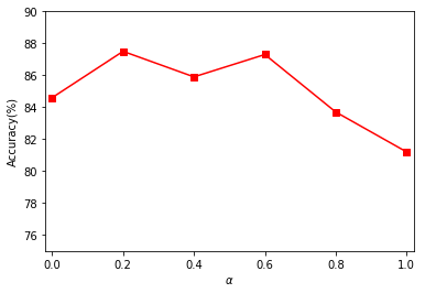
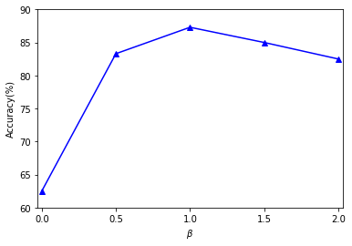
Parameter Sensitivity Analysis: We testify the sensitivity of our model to parameters $\alpha$ and $\beta$, i.e. the hyper-parameters for label-classification loss and domain cross-entropy loss. As an illustration, we use task $\textbf{A}\rightarrow\textbf{W}$ to report the transfer accuracy of DART with different choice of $\alpha$ and $\beta$. Figure 5(c) reports the accuracy of varying $\alpha\in\{0.0,0.2,0.6,0.8,1.0\}$ while fixing $\beta=1.0$. We observe that DART achieves the best performance when $\alpha$ is set from [0.2,0.6], although there is a vibration when $\alpha=0.4$. The vibration may be caused by the small number of samples. As for $\beta$, the best accuracy can be obtained when setting $\beta$ from $[0.5,1.5]$, illustrating a bell-shaped curve as showed in Figure 5(d).

References

- Ben-David et al. [2009] Shai Ben-David, John Blitzer, Koby Crammer, Alex Kulesza, Fernando Pereira, and Jennifer Wortman Vaughan. A theory of learning from different domains. Machine Learning, 79:151–175, 2009.
- Bousmalis et al. [2016] Konstantinos Bousmalis, George Trigeorgis, Nathan Silberman, Dilip Krishnan, and Dumitru Erhan. Domain separation networks. In NIPS, 2016.
- Bousmalis et al. [2017] Konstantinos Bousmalis, Nathan Silberman, David Dohan, Dumitru Erhan, and Dilip Krishnan. Unsupervised pixel-level domain adaptation with generative adversarial networks. In 2017 IEEE Conference on Computer Vision and Pattern Recognition, CVPR 2017, Honolulu, HI, USA, July 21-26, 2017, pages 95–104, 2017.
- Denker et al. [1988] John S. Denker, W. R. Gardner, Hans Peter Graf, Donnie Henderson, Richard E. Howard, Wayne E. Hubbard, Lawrence D. Jackel, Henry S. Baird, and Isabelle Guyon. Neural network recognizer for hand-written zip code digits. In NIPS, 1988.
- Donahue et al. [2014] Jeff Donahue, Yangqing Jia, Oriol Vinyals, Judy Hoffman, Ning Zhang, Eric Tzeng, and Trevor Darrell. Decaf: A deep convolutional activation feature for generic visual recognition. In ICML, 2014.
- Ganin and Lempitsky [2015] Yaroslav Ganin and Victor S. Lempitsky. Unsupervised domain adaptation by backpropagation. In ICML, 2015.
- Ganin et al. [2016] Yaroslav Ganin, Evgeniya Ustinova, Hana Ajakan, Pascal Germain, Hugo Larochelle, François Laviolette, Mario Marchand, and Victor Lempitsky. Domain-adversarial training of neural networks. Journal of Machine Learning Research, 17(59):1–35, 2016.
- Gong et al. [2012] Boqing Gong, Yuan Shi, Fei Sha, and Kristen Grauman. Geodesic flow kernel for unsupervised domain adaptation. 2012 IEEE Conference on Computer Vision and Pattern Recognition, pages 2066–2073, 2012.
- Goodfellow et al. [2014] Ian J. Goodfellow, Jean Pouget-Abadie, Mehdi Mirza, Bing Xu, David Warde-Farley, Sherjil Ozair, Aaron C. Courville, and Yoshua Bengio. Generative adversarial nets. In NIPS, 2014.
- Grandvalet and Bengio [2004] Yves Grandvalet and Yoshua Bengio. Semi-supervised learning by entropy minimization. In NIPS, 2004.
- Gretton et al. [2006] Arthur Gretton, Karsten M. Borgwardt, Malte J. Rasch, and Bernhard. A kernel method for the two-sample-problem. In NIPS, 2006.
- He et al. [2016] Kaiming He, Xiangyu Zhang, Shaoqing Ren, and Jian Sun. Deep residual learning for image recognition. 2016 IEEE Conference on Computer Vision and Pattern Recognition (CVPR), pages 770–778, 2016.
- LeCun et al. [1998] Yann LeCun, Léon Bottou, Yoshua Bengio, and Patrick Haffner. Gradient-based learning applied to document recognition. Proceedings of the IEEE, 86(11):2278–2324, 1998.
- Lin et al. [2014] Tsung-Yi Lin, Michael Maire, Serge J. Belongie, James Hays, Pietro Perona, Deva Ramanan, Piotr Dollár, and C. Lawrence Zitnick. Microsoft coco: Common objects in context. In ECCV, 2014.
- Liu and Tuzel [2016] Ming-Yu Liu and Oncel Tuzel. Coupled generative adversarial networks. In NIPS, 2016.
- Liu et al. [2017] Ming-Yu Liu, Thomas Breuel, and Jan Kautz. Unsupervised image-to-image translation networks. CoRR, abs/1703.00848, 2017.
- Long et al. [2013] Mingsheng Long, Jianmin Wang, Guiguang Ding, Jia-Guang Sun, and Philip S. Yu. Transfer feature learning with joint distribution adaptation. 2013 IEEE International Conference on Computer Vision, pages 2200–2207, 2013.
- Long et al. [2015] Mingsheng Long, Yue Cao, Jianmin Wang, and Michael I. Jordan. Learning transferable features with deep adaptation networks. In ICML, 2015.
- Long et al. [2016] Mingsheng Long, Han Zhu, Jianmin Wang, and Michael I. Jordan. Unsupervised domain adaptation with residual transfer networks. In NIPS, 2016.
- Long et al. [2017] Mingsheng Long, Jianmin Wang, and Michael I. Jordan. Deep transfer learning with joint adaptation networks. In ICML, 2017.
- Long et al. [2018] Mingsheng Long, ZHANGJIE CAO, Jianmin Wang, and Michael I Jordan. Conditional adversarial domain adaptation. In S. Bengio, H. Wallach, H. Larochelle, K. Grauman, N. Cesa-Bianchi, and R. Garnett, editors, Advances in Neural Information Processing Systems 31, pages 1647–1657. 2018.
- Mansour et al. [2009] Yishay Mansour, Mehryar Mohri, and Afshin Rostamizadeh. Domain adaptation: Learning bounds and algorithms. In In Proceedings of COLT. Citeseer, 2009.
- Pan and Yang [2010] Sinno Jialin Pan and Qiang Yang. A survey on transfer learning. IEEE Transactions on Knowledge and Data Engineering, 22:1345–1359, 2010.
- Pan et al. [2009] Sinno Jialin Pan, Ivor W. Tsang, James T. Kwok, and Qiang Yang. Domain adaptation via transfer component analysis. IEEE Transactions on Neural Networks, 22:199–210, 2009.
- Pan et al. [2017] Yingwei Pan, Ting Yao, Houqiang Li, and Tao Mei. Video captioning with transferred semantic attributes. In 2017 IEEE Conference on Computer Vision and Pattern Recognition, CVPR 2017, Honolulu, HI, USA, July 21-26, 2017, pages 984–992, 2017.
- Russakovsky et al. [2015] Olga Russakovsky, Jia Deng, Hao Su, Jonathan Krause, Sanjeev Satheesh, Sean Ma, Zhiheng Huang, Andrej Karpathy, Aditya Khosla, Michael S. Bernstein, Alexander C. Berg, and Li Fei-Fei. Imagenet large scale visual recognition challenge. International Journal of Computer Vision, 115:211–252, 2015.
- Saenko et al. [2010] Kate Saenko, Brian Kulis, Mario Fritz, and Trevor Darrell. Adapting visual category models to new domains. In ECCV, 2010.
- Sun and Saenko [2016] Baochen Sun and Kate Saenko. Deep coral: Correlation alignment for deep domain adaptation. In ECCV Workshops, 2016.
- Taigman et al. [2016] Yaniv Taigman, Adam Polyak, and Lior Wolf. Unsupervised cross-domain image generation. CoRR, abs/1611.02200, 2016.
- Tzeng et al. [2014] Eric Tzeng, Judy Hoffman, Ning Zhang, Kate Saenko, and Trevor Darrell. Deep domain confusion: Maximizing for domain invariance. CoRR, abs/1412.3474, 2014.
- Tzeng et al. [2017] Eric Tzeng, Judy Hoffman, Kate Saenko, and Trevor Darrell. Adversarial discriminative domain adaptation. CoRR, abs/1702.05464, 2017.
- Wang and Deng [2018] Mei Wang and Weihong Deng. Deep visual domain adaptation: A survey. Neurocomputing, 312:135–153, 2018.
- Zhuo et al. [2017] Junbao Zhuo, Shuhui Wang, Weigang Zhang, and Qingming Huang. Deep unsupervised convolutional domain adaptation. In Proceedings of the 2017 ACM on Multimedia Conference, MM ’17, pages 261–269, 2017. ISBN 978-1-4503-4906-2.