Interference-Free Transceiver Design and Signal Detection for Ambient Backscatter Communication Systems over Frequency-Selective ChannelsThanks: C. Zhang is with Beijing Intelligent Logistics System Collaborative Innovation Center and School of Electronic and Information Engineering, Beijing Jiaotong University, Beijing 100044, P. R. China (email: 15212111@bjtu.edu.cn).Thanks: G. Wang is with Beijing Key Lab of Transportation Data Analysis and Mining, School of Computer and Information Technology, Beijing Jiaotong University, Beijing 100044, P. R. China (e-mails: gpwang@bjtu.edu.cn).Thanks: F. Gao is with Department of Automation, Tsinghua University, State Key Lab of Intelligent Technologies and Systems, Tsinghua National Laboratory for Information Science and Technology (TNList) Beijing 100084, P. R. China (email: feifeigao@ieee.org).Thanks: P. D. Diamantoulakis and G. K. Karagiannidis are with the Department of Electrical and Computer Engineering, Aristotle University of Thessaloniki, Thessaloniki 54124, Greece (e-mails: padiaman, geokarag@auth.gr).Thanks: Corresponding author: Gongpu Wang (gpwang@bjtu.edu.cn).

Chong Zhang Gongpu Wang Panagiotis D. Diamantoulakis Feifei Gao George K. Karagiannidis Affiliation:

Abstract

In this letter, we study the ambient backscatter communication systems over frequency-selective channels. Specifically, we propose an interference-free transceiver design to facilitate signal detection at the reader. Our design utilizes the cyclic prefix (CP) of orthogonal frequency-division multiplexing (OFDM) source symbols, which can cancel the signal interference and thus enhance the detection accuracy at the reader. Meanwhile, our design results in no interference on the existing OFDM communication systems. We also suggest a maximum likelihood (ML) detector for the reader and derive two detection thresholds. Simulations are then provided to corroborate our proposed studies.

Index Terms:

Ambient backscatter, frequency-selective channels, signal detection, wireless communications.

I Introduction

As a newborn green technology for the Internet of Things (IoT), ambient backscatter [1], has attracted extensive attention [2, 3, 4, 5]. This novel technology utilizes ambient radio frequency (RF) signals to implement the backscatter communications of low data-rate devices such as tags or sensors, and is able to free them from batteries.

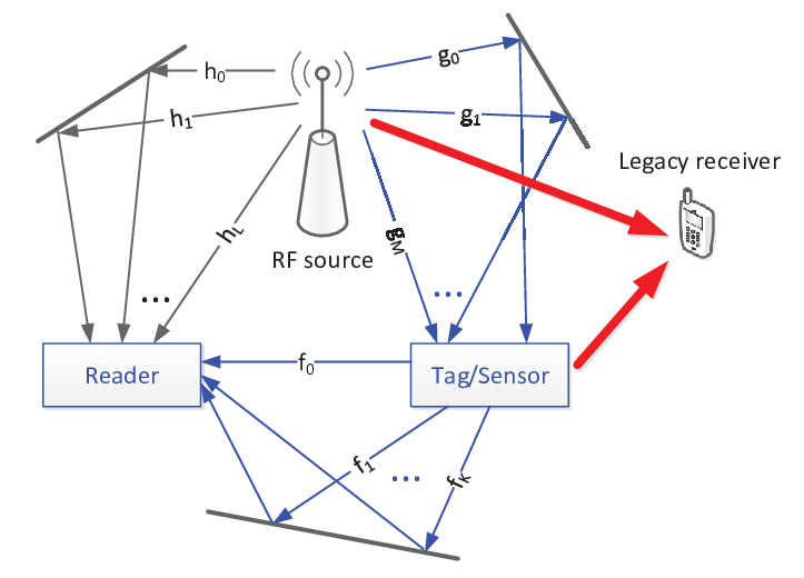
A typical ambient backscatter communication system includes three components: a RF source, a tag (or a sensor), and a reader, as shown in Fig. 1. The communication process between the tag and the reader mainly contains two steps: first, the tag harvests energy from the signals of the RF source; second, the tag modulates its binary information onto the received RF signals and then backscatters them to the reader.

In the open literature, almost all studies about ambient backscatter communication are based on the assumption of flat-fading channels. Nevertheless, the frequency-selective channels widely exist in numerous application scenarios. For ambient backscatter communication systems, frequency-selective channels could lead to multiple copies of backscattered signals at the reader, together with multiple copies of source signals. Consequently, it is one challenging problem for the reader to realize recovery of tag binary information.

In this letter, we investigate the ambient backscatter communication systems over frequency-selective channels and propose an interference-free transceiver design to cope with the signal detection challenge at the reader. In our proposed design, the cyclic prefix (CP) structure of orthogonal frequency-division multiplexing (OFDM) source symbols is exploited, which can benefit signal detection at the reader via cancelling the signal interference. Meanwhile, different from the transceiver design in [4], our design leads to no interference to the legacy receivers. Next, a maximum likelihood (ML) detector is proposed and two detection thresholds are derived. Our simulation results show that our transceiver design for the frequency-selective channels is efficient and achieves low bit error rate (BER) due to interference cancellation.

Refer to caption — Fig. 1: System model.

The rest of this paper is organized as follows: Section II formulates the model of the ambient backscatter communication system over frequency-selective channels. Section III proposes the transceiver design and Section IV derives the ML detector with two detection thresholds. Section V provides the simulation results and finally Section VI summarizes this letter.

II System Model

Consider an ambient backscatter communication system over frequency-selective channels in Fig. 1. The multi-path channels between the RF source and reader, the RF source and tag, the reader and tag are denoted by $h_{l}\,\,(l=0,1,\cdots,L)$ , $g_{m}\,\,(m=0,1,\cdots,M)$ , $f_{k}\,\,(k=0,1,\cdots,K)$ , separately. Both the reader and the legacy receiver can receive signals from the RF source and the tag over frequency-selective channels.

The signal transmitted by the RF source is $s(n)$ with a zero-mean and a variance of $P_{s}$ and $s(n)\sim\mathcal{CN}(0,P_{s})$ . Due to the multi-path channels $g(m)\,\,(m=0,1,\cdots,M)$ , the signal arriving at the tag antenna can be given as

\displaystyle x(n)=\sum_{m=0}^{M}g_{m}s(n-m).

(1)

The tag next modulates its own binary signal $B(n)$ onto the received signal $x(n)$ to communicate with the reader via backscattering $x(n)$ or not. Specifically, the tag changes its antenna impedance to reflect $x(n)$ to the reader so as to indicate $B(n)=1$ ; and when indicating $B(n)=0$ , the tag switches the impedance to a certain value so that no signal can be reflected. Suppose that the tag information $B(n)=0$ and $B(n)=1$ are equally probable.

Finally, the received signal at the reader can be expressed as

\displaystyle y(n)=\sum_{l=0}^{L}h_{l}s(n-l)+\eta\sum_{k=0}^{K}f_{k}B(n-k)x(n-k)+w(n),

(2)

where $\eta$ represents the complex attenuation inside the tag, $w(n)$ denotes the additive white Gaussian noise (AWGN) and we assume $w(n)\sim\mathcal{CN}(0,N_{w})$ .

III Interference-free Transceiver Design

In this section, we describe an interference-free transceiver design, whose implementation mainly consists of three crucial aspects: the tag signal design, the signal interference cancelling method, and the discrete Fourier transformation (DFT) operation.

III-A Tag Signal Design

With the assumption that the RF source emits OFDM symbols, the signal structure in one OFDM symbol period at the tag is presented in Fig. 2. We set $C$ and $N$ as the lengths of the CP and the effective part of OFDM symbol, respectively. The parameter $Q$ is defined as $Q={\rm max}\{L,M,K\}$ .

Obviously, both $s(n)$ and $x(n)$ have repeating sequences, even if the signal $x(n)$ experiences the multi-path channels $g(m)\,\,(m=0,1,\cdots,M)$ . Besides, we divide one OFDM symbol period into four phases for the designed tag signal $B(n)$ . In Phase 1, Phase 3, and Phase 4, no received signal $x(n)$ will be reflected, i.e., $B(n)=0$ . In this case, the signals arriving at the reader directly come from the RF source. However, in Phase 2, the tag modulates its binary data onto the signal $x(n)$ from the time $Q$ to the time $C-K-1$ while no signal is backscattered to the reader in the rest of the Phase 2. By exploiting the signals arriving at the reader in Phase 2 and Phase 4, we can cancel the signal interference, which will be presented in the next subsection.

Remark 1

It can be checked from Fig. 2 that the signal structure of $B(n)$ solely effects the samples in the CP of the OFDM symbol. Since the CP will be removed at the legacy receiver, this transceiver design at the tag will lead to no interference to the legacy receivers.

III-B Signal Interference Cancelling Method

Denote the received signals at the reader in Phase 2 and Phase 4 as $y_{1}(n)\,\,\,(n=Q,\cdots,C-1)$ and $y_{2}(n)\,\,\,(n=N+Q,\cdots,N+C-1)$ , respectively. We can obtain

$\displaystyle y_{1}(n)=$	$\displaystyle\sum_{l=0}^{L}h_{l}s(n-l)+\eta\sum_{k=0}^{K}f_{k}B(n-k)x(n-k)$
	$\displaystyle\qquad\qquad\qquad\qquad\qquad\qquad\qquad+w_{1}(n),$	(3)
$\displaystyle y_{2}(n)=$	$\displaystyle\sum_{l=0}^{L}h_{l}s(n-l)+w_{2}(n),$	(4)

where $w_{1}(n)$ and $w_{2}(n)$ are both AWGN. Assume that $w_{1}(n)\sim\mathcal{CN}(0,N_{w})$ and $w_{2}(n)\sim\mathcal{CN}(0,N_{w})$ .

Apparently, the term $\sum_{l=0}^{L}h_{l}s(n-l)$ in (III-B) and (4) carries no tag binary information and thus is the interference for the tag signal recovery at the reader, which can be cancelled for further improvement of detection accuracy.

Signal interference cancelling is implemented via subtracting $y_{2}(n)$ from $y_{1}(n)$ , thus the received signals can be written as

$\displaystyle z(n)=$	$\displaystyle y_{1}(n+Q)-y_{2}(n+N+Q)$
$\displaystyle=$	$\displaystyle\eta\sum_{k=0}^{K}f_{k}B(n-k)x(n-k)+w_{1}(n)-w_{2}(n),$
$\displaystyle=$	$\displaystyle\eta\sum_{k=0}^{K}f_{k}B(n-k)x(n-k)+w_{e}(n),$	(5)

where $n=0,1,\cdots,C-Q-1$ and $w_{e}(n)\sim\mathcal{CN}(0,2N_{w})$ .

III-C DFT Operation

Assume $T=C-Q-1$ and $R=C-Q-K-1$ . After signal interference cancelling at the reader, let us construct the signal vector z as

	$\displaystyle\textbf{z}=$	$\displaystyle[z(0)+z(R+1),\cdots,z(T-R-1)+z(T),$
		$\displaystyle\qquad\qquad\,\,\,\,\,z(T-R-1),\cdots,z(R-1),z(R)]^{\rm T}.$		(6)

Define

$\displaystyle\textbf{b}=$	$\displaystyle[B(0),B(1),\cdots,B(n),\cdots,B(R)],$	(7)
$\displaystyle\textbf{x}=$	$\displaystyle[x(0),x(1),\cdots,x(n),\cdots,x(R)]^{\rm T},$	(8)
$\displaystyle\textbf{w}=$	$\displaystyle[w_{e}(0)+w_{e}(R+1),\cdots,w_{e}(T-R-1)+w_{e}(T),$
	$\displaystyle\qquad\qquad\;\,w_{e}(T-R-1),\cdots,w_{e}(R-1),w_{e}(R)]^{\rm T}.$	(9)

Denote F as the $(R+1)\times(R+1)$ DFT matrix with the $(p,q)$ th element $\textbf{F}_{pq}=\exp(-j2\pi pq/(R+1))$ . Let us consider a Toeplitz matrix T, which possesses the first row of $\textbf{t}_{\textbf{r}}=[f_{0},0,\cdots,0,f_{K},f_{K-1},\cdots,f_{k},\cdots,f_{1}]$ and the first column of $\textbf{t}_{\textbf{c}}=[f_{0},f_{1},\cdots,f_{k},\cdots,f_{K},0,\cdots,0]^{\rm T}$ .

Consequently, we reconstruct the signal vector z based on DFT as, i.e., DFT outputs $\tilde{\textbf{z}}$

$\displaystyle\tilde{\textbf{z}}=$	Fz
$\displaystyle=$	$\displaystyle\,\eta\textbf{F}\textbf{T}\cdot{\rm diag}[\textbf{b}]\cdot\textbf{x}+\textbf{F}\textbf{w}$
$\displaystyle=$	$\displaystyle\,\eta\cdot{\rm diag}\left[\tilde{\textbf{f}}^{\rm T}\right]\cdot{\rm diag}[\textbf{b}]\cdot\tilde{\textbf{x}}+\tilde{\textbf{w}},$	(10)

where

$\displaystyle\tilde{\textbf{z}}=\,$	$\displaystyle[\tilde{z}(0),\tilde{z}(1),\cdots,\tilde{z}(n),\cdots,\tilde{z}(R)]^{\rm T}=\textbf{F}\textbf{z},$	(11)
$\displaystyle\tilde{\textbf{x}}=\,$	$\displaystyle[\tilde{x}(0),\tilde{x}(1),\cdots,\tilde{x}(n),\cdots,\tilde{x}(R)]^{\rm T}=\textbf{F}\textbf{x},$	(12)
$\displaystyle\tilde{\textbf{w}}=\,$	$\displaystyle[\tilde{w}_{e}(0),\tilde{w}_{e}(1),\cdots,\tilde{w}_{e}(n),\cdots,\tilde{w}_{e}(R)]^{\rm T}=\textbf{F}\textbf{w},$	(13)
$\displaystyle\tilde{\textbf{f}}=\,$	$\displaystyle[\tilde{f}_{0},\tilde{f}_{1},\cdots,\tilde{f}_{n},\cdots,\tilde{f}_{R}]^{\rm T}=\textbf{F}\textbf{t}_{\textbf{r}}^{\rm T}.$	(14)

According to the central limit theorem (CLT), we can have $\tilde{x}(n)\sim\mathcal{N}(0,P_{x})$ , $\tilde{w}_{e}(n)\sim\mathcal{N}(0,P_{w})$ and $\tilde{f}_{n}\sim\mathcal{N}(0,P_{f})$ , where

$\displaystyle P_{x}=$	$\displaystyle(R+1)P_{s}\sum_{m=0}^{M}\|g_{m}\|^{2},$	(15)
$\displaystyle P_{w}=$	$\displaystyle 2(T+1)N_{w},$	(16)
$\displaystyle P_{f}=$	$\displaystyle\sum_{k=0}^{K}\|f_{k}\|^{2}.$	(17)

IV Signal Detection at the Reader

In this section, the ML detector together with two detection thresholds: the optimal threshold and the equiprobable error threshold, is derived. Moreover, the bit error rate (BER) expression is obtained for performance analysis.

IV-A ML Detector

Due to the lower data-rate of the tag signal $B(n)$ than that of the signal $\tilde{z}(n)$ , we suppose the signal $B(n)$ remains equivalent within $W$ samples of $\tilde{z}(n)$ . Let us construct the test statistic as

\displaystyle\Gamma_{t}=\frac{1}{W}\sum_{n=(t-1)W+1}^{tW}\left|\tilde{z}(n)\right|^{2},

(18)

where $t=1,2,\cdots,T$ , and $\tilde{z}(n)$ is expanded as

\displaystyle\tilde{z}(n)=\left\{\begin{aligned} &\tilde{w}(n),&{\rm if}\,\,\,B(n)=0,\\ &\eta\tilde{f}_{n}\tilde{x}(n)+\tilde{w}(n),&{\rm if}\,\,\,B(n)=1.\\ \end{aligned}\right.

(19)

Define

	$\displaystyle U=$	$\displaystyle\|\eta\|^{2}P_{x}P_{f}=(R+1)\|\eta\|^{2}P_{s}\sum_{m=0}^{M}\|g_{m}\|^{2}\sum_{k=0}^{K}\|f_{k}\|^{2},$		(20)
	$\displaystyle V=$	$\displaystyle P_{w}=2(T+1)N_{w}.$		(21)

Thus, the test statistic $\Gamma_{t}$ is subjected to [2, 4]

\displaystyle\Gamma_{t}\sim\left\{\begin{aligned} &\mathcal{N}\left(V,\frac{V^{2}}{W}\right),&{\rm if}\,\,\,B(n)=0.\\ &\mathcal{N}\left(U+V,\frac{(U+V)^{2}}{W}\right),&{\rm if}\,\,\,B(n)=1.\\ \end{aligned}\right.

(22)

The ML detector can be made as

\displaystyle\hat{B}(n)=\mathop{\arg\max}\limits_{B(n)\in\{0,1\}}{\rm Pr}(\Gamma_{t}|B(n)),

(23)

where ${\rm Pr}(\Gamma_{t}|B(n))$ is the probability density function (PDF) of $\Gamma_{t}$ given $B(n)$ .

IV-B Optimal Threshold

The optimal threshold $T^{{\rm opt}}_{h}$ of the ML detector must satisfy

\displaystyle{\rm Pr}(\Gamma_{t}|B(n)=0)={\rm Pr}(\Gamma_{t}|B(n)=1).

(24)

The solution to (24) is derived as

\displaystyle T^{{\rm opt}}_{h}=\frac{V(U+V)+\sqrt{V^{2}(U+V)^{2}+(2+4V/U)\frac{\ln{(1+U/V)}}{W}}}{U+2V}.

(25)

Thus, the detection rule is

\displaystyle\hat{B}(n)=\left\{\begin{matrix}0,&{\rm if}\,\,\,\Gamma_{t}<T^{{\rm opt}}_{h},\\ 1,&{\rm if}\,\,\,\Gamma_{t}>T^{{\rm opt}}_{h}.\end{matrix}\right.

(26)

IV-C BER Performance

Define $p_{0}={\rm Pr}(B(n)=1|B(n)=0)$ and $p_{1}={\rm Pr}(B(n)=0|B(n)=1)$ . The BER of the ML detector is given by

	$\displaystyle P_{e}=$	$\displaystyle{\rm Pr}(B(n)=0)p_{0}+{\rm Pr}(B(n)=1)p_{1}$
	$\displaystyle=$	$\displaystyle\frac{1}{2}\left(p_{0}+p_{1}\right).$		(27)

Given the detection threshold $T^{{\rm opt}}_{h}$ , there is

\displaystyle P_{e}=\frac{1}{2}+\frac{1}{2}Q\left(\frac{T^{{\rm opt}}_{h}-V}{\sqrt{\frac{V^{2}}{W}}}\right)-\frac{1}{2}Q\left(\frac{T^{{\rm opt}}_{h}-U-V}{\sqrt{\frac{(U+V)^{2}}{W}}}\right),

(28)

where

\displaystyle Q(x)=\frac{1}{\sqrt{2\pi}}\int_{x}^{\infty}{\rm e}^{-\frac{t^{2}}{2}}{\rm d}t.

(29)

IV-D Equiprobable Error Threshold

In this subsection, we discuss the detection threshold that can obtain the same error probability for $B(n)=0$ and $B(n)=1$ , i.e., $p_{0}=p_{1}$ [2].

We can further derive the equation $p_{0}=p_{1}$ as

\displaystyle Q\left(\frac{T^{{\rm equ}}_{h}-V}{\sqrt{\frac{V^{2}}{W}}}\right)=Q\left(\frac{U+V-T^{{\rm equ}}_{h}}{\sqrt{\frac{(U+V)^{2}}{W}}}\right),

(30)

where $T^{{\rm equ}}_{h}$ is the equiprobable error threshold.

Here, we construct the approximation of the Q-function [6]:

\displaystyle Q(x)\approx\frac{{\rm e}^{-bx-ax^{2}}}{2},\,\,a=0.416,\,\,b=0.717.

(31)

Utilizing this approximation in (30) and exerting some mathematical manipulations, one obtains the detection threshold $T^{{\rm equ}}_{h}$ as

\displaystyle T^{{\rm equ}}_{h}=\frac{-\varsigma_{1}+\sqrt{\varsigma^{2}_{1}-4\varsigma_{0}\varsigma_{2}}}{2\varsigma_{0}},

(32)

where

$\displaystyle\varsigma_{0}=$	$\displaystyle\frac{a\sqrt{W}(U^{2}+2UV)}{V(U+V)},$	(33)
$\displaystyle\varsigma_{1}=$	$\displaystyle b(U+2V)-2a\sqrt{W}U,$	(34)
$\displaystyle\varsigma_{2}=$	$\displaystyle-2bV(U+V).$	(35)

V Simulation Results

In this section, numerical results are provided to assess the BER performance of the ML detector. All the channels follow Gaussian distributions with zero-mean and unit-variance. We set the three parameters $L$ , $M$ and $K$ as $L=M=K=8$ . The attenuation $\eta$ and the noise variance $N_{w}$ are fixed as $0.5$ and $1$ , separately. We exert $10^{7}$ Monte Carlo trials for every experiment.

Fig. 3 plots the BER curves versus signal-to-noise ratio (SNR) for the ML detector with two different thresholds. Two different numbers of averaging samples $W$ , i.e., $W=8$ and $W=10$ , are adopted, and the length of CP is set to 256. As seen, the simulation results keep consistent with analysis results. Besides, the BER performance is enhanced with enlarging SNR.

Fig. 4 depicts the BER curves versus the number of averaging samples $W$ for three different SNR, i.e., SNR=15 dB, SNR=20 dB and SNR=25 dB. We fix the length of CP $C$ as 256. It is found that the BER performance is improved with increasing $W$ .

VI Conclusion

This letter investigated the ambient backscatter communication systems over frequency-selective channels and proposed an interference-free transceiver design to cope with the signal detection challenge at the reader. The CP structure of OFDM symbols was exploited to cancel the signal interference at the reader and meanwhile our design led to no interference to legacy receivers. Finally, a ML detector with two thresholds was derived and its BER expression was obtained. Simulation results corroborated that our transceiver design fitted the scenario of frequency-selective channels and achieved low bit error rate (BER) due to interference cancellation.

References

[1] N. V. Huynh, D. T. Hoang, X. Lu, D. Niyato, P. Wang, and D. I. Kim, “Ambient backscatter communications: a contemporary survey,” IEEE Commun. Surveys Tuts., vol. 20, no. 4, pp. 2889-2922, 4th Quart., 2018.
[2] G. Wang, F. Gao, R. Fan, and C. Tellambura, “Ambient backscatter communication systems: detection and performance analysis,” IEEE Trans. Commun., vol. 64, no. 11, pp. 1-10, Aug. 2016.
[3] J. Qian, F. Gao, G. Wang, S. Jin, and H. Zhu, “Noncoherent detections for ambient backscatter system,” IEEE Trans. Wireless Commun., vol. 16, no. 3, pp. 1412-1422, Mar. 2017.
[4] G. Yang, Y. C. Liang, R. Zhang, and Y. Pei, “Modulation in the air: backscatter communication over ambient OFDM carrier,” IEEE Trans. Commun., vol. 66, no. 3, pp. 1219-1233, Mar. 2018.
[5] G. Yang, Q. Zhang, and Y. Liang, “Cooperative ambient backscatter communications for green Internet-of-Things,” IEEE Internet Things J., vol. 5, no. 2, pp. 1116-1130, Apr. 2018.
[6] J. T. Lin, “Approximating the normal tail probability and its inverse for use on a pocket calculator,” Appl. Statis., vol. 38, no. 1, pp. 69-70, Jan. 1989.