Meronic Einstein-Yang-Mills black hole in 5D and gravitational spin from isospin effect

We will consider the usual spherically symmetric ansatz for the five-dimensional space-time metric:

$$ds^{2}=-f^{2}(r)dt^{2}+\frac{1}{f^{2}(r)}dr^{2}+\frac{r^{2}}{4}d\Omega_{S^{3}}^{2}\,,$$

(6)

where $t$ stands for the time coordinate, $r$ corresponds to the radial coordinate, and $d\Omega_{S^{3}}^{2}$ denotes the line element of the unit three-sphere. The group $SU(2)$ is diffeomorphic to $S^{3}$. Therefore $d\Omega^{2}_{S^{3}}$ can be written as (see Appendix A)

$$d\Omega^{2}_{S^{3}}=-\frac{1}{2}\mathrm{Tr}[dUU^{-1}\otimes dUU^{-1}]\,,$$

(7)

where $dUU^{-1}=-i\omega_{R}^{a}t_{a}$ corresponds to the right-invariant Maurer-Cartan form on $SU(2)$, and whose components satisfy

$$d\omega_{R}^{a}=\frac{1}{2}\epsilon^{a}_{\;bc}\omega_{R}^{b}\wedge\omega_{R}^{c}\,.$$

(8)

For the gauge field we will consider Meron-like configurations, i.e., connection one-forms $A=A_{\mu}dx^{\mu}$ that are proportional to a pure gauge field deAlfaro:1976qet. According to (5) this means

$$A=-\lambda dUU^{-1}\quad,\quad\lambda\neq 0,1,$$

(9)

which is equivalent to

$$A=i\lambda\omega_{R}^{a}t_{a}\,.$$

(10)

The corresponding curvature two-form is given by $F=dA+A\wedge A=\frac{1}{2}F_{\mu\nu}dx^{\mu}dx^{\nu}$. For a gauge field of the form (10) it takes the simple form

$$F=\frac{\lambda-1}{2\lambda}\left[A,A\right]\,.$$

(11)

In the case of a Meron gauge field, Yang-Mills equations (4) can be easily solved when written in terms of forms:

$$d*F+[A,*F]=0\,,$$

(12)

where $*F$ denotes the Hodge dual of $F$. In the following, it will prove convenient to define a set of fünfbeins $e^{A}$, $A=0,\ldots,4$, such that $ds^{2}=\eta_{AB}e^{A}e^{B}$ with $\eta_{AB}=\mathrm{diag}\left(-,+,+,+,+\right)$. The natural choice is

	$\displaystyle e^{0}$	$\displaystyle=f(r)dt\,,$
	$\displaystyle e^{1}$	$\displaystyle=\frac{1}{f(r)}dr\,,$		(13)
	$\displaystyle e^{a+1}$	$\displaystyle=\frac{r}{2}\omega_{R}^{a}\,.$

The gauge connection (10) can be written in terms of the angular fünfbeins as

$$A=\frac{2i\lambda}{r}e^{a+1}t_{a}\,.$$

(14)

Therefore, in the fünfbein basis $A=A_{A}e^{A}$, the components of the Meron gauge field take the simple form

$$A_{A}=\frac{2i\lambda}{r}\delta_{A}^{a+1}t_{a}\,.$$

(15)

Similarly, the curvature two-form (11) can be written in terms of the fünfbein basis as $F=\frac{1}{2}F_{AB}e^{A}\wedge e^{B}$, with components

$$F_{AB}=-\frac{4i\lambda\left(\lambda-1\right)}{r^{2}}\epsilon_{\;bc}^{a}\delta_{A}^{b+1}\delta_{B}^{c+1}t_{a}\,.$$

(16)

The Hodge dual of $F$, on the other hand, takes the form

$$*F=-\frac{4i\lambda\left(\lambda-1\right)}{r^{2}}\,t_{a}\,e^{0}\wedge e^{1}\wedge e^{a+1}\,.$$

(17)

Using (13) and (17), equation (12) reduces to

$$\frac{2i\lambda\left(\lambda-1\right)}{r}\left(d\omega_{R}^{a}-\lambda\epsilon_{\;bc}^{a}\omega_{R}^{b}\wedge\omega_{R}^{c}\right)\,t_{a}\;e^{0}\wedge e^{1}=0\,,$$

(18)

which, due to the Maurer Cartan equation (8), is solved for

$$\lambda=\frac{1}{2}\ .$$

(19)

The group element $U\in SU(2)$ that corresponds to the Meron gauge potential (9) can be explicitly written using the generalized hedgehog ansatz Canfora:2013mrh. It is interesting to note that such an approach (subsequently worked out in Canfora:2013osa; Canfora:2013xja; Canfora:2014aia; Canfora:2014jka; Chen:2013qha; Canfora:2015xra; Chen:2015bek; Ayon-Beato:2015eca; Canfora:2014jsa; Canfora:2015hxa; Canfora:2016spb; Tallarita:2017bks; Canfora:2017ivv; Canfora:2017gno; Canfora:2017yio) was originally developed to analyze the Skyrme and Einstein-Skyrme models, but it also works in the case of Yang-Mills and Einstein-Yang-Mills theories with almost no modifications (as one can see comparing Canfora:2013osa, Ayon-Beato:2015eca with Canfora:2012ap, Canfora:2017yio). This approach is specially designed for situations in which the group element cannot be deformed continuously to the identity.

In order to write down the ansatz for $U$, we adopt the standard parametrization for $SU(2)$ elements:

$$U(x^{\mu})=e^{-i\alpha^{a}t_{a}}=\mathrm{cos}\frac{\alpha}{2}(x^{\mu})\mathbb{\mathbf{I}}-2in^{a}t_{a}\,\mathrm{sin}\frac{\alpha}{2}(x^{\mu})\,,$$

(20)

where $\mathbb{\mathbf{I}}$ is the $2\times 2$ identity and $n^{a}$ is a unit vector that can be written in the form

$$n^{1}=\mathrm{sin}\Theta\mathrm{cos}\Phi\,\,\,,\,\,\,n^{2}=\mathrm{sin}\Theta\mathrm{sin}\Phi\,\,\,,\,\,\,n^{3}=\mathrm{cos}\Theta\,\,.$$

(21)

The generalized hedgehog ansatz corresponds to the following choice for the functions $\alpha$, $\Theta$, $\Phi$ in terms of Euler variables:

$$\Phi=\frac{\varphi-\psi}{2}\ ,\ \ \tan\Theta=\tan\dfrac{\theta}{2}\csc\dfrac{\varphi+\psi}{2}\,,\ \ \cot\frac{\alpha}{2}=\sec\Theta\tan\frac{\varphi+\psi}{2}\ .$$

(22)

This leads to the following form for the components of the right-invariant Maurer-Cartan form on SU(2):

	$\displaystyle\omega_{R}^{1}$	$\displaystyle=-\mathrm{sin}\psi d\theta+\mathrm{cos}\psi\,\mathrm{sin}\theta d\varphi\,,$
	$\displaystyle\omega_{R}^{2}$	$\displaystyle=\mathrm{cos}\psi d\theta+\mathrm{sin}\psi\,\mathrm{sin}\theta d\varphi\,,$		(23)
	$\displaystyle\omega_{R}^{3}$	$\displaystyle=d\psi+\mathrm{cos}\theta d\varphi\,,$

$$0\leq\psi<4\pi\,,\,\,0\leq\theta<\pi\,,\,\,0\leq\varphi<2\pi\,,$$

(24)

which clearly satisfy (8). Using (23), and defining the coordinates $x^{m}=\left\{\psi,\theta,\phi\right\}$, the metric for the three-sphere (7) takes the form

$$d\Omega_{S^{3}}^{2}=h_{mn}dx^{m}dx^{n}\;,\quad h_{mn}=\frac{1}{4}\left(\begin{array}[]{ccc}1&0&\cos\theta\\ 0&1\\ \cos\theta&0&1\end{array}\right)\,.$$

(25)

while the components of the gauge field (10) read

$$\begin{array}[]{lcl}&&A_{t}=A_{r}=0\,,\\[5.0pt] &&A_{\psi}=\dfrac{i}{2}\,t_{3}\,,\\[5.0pt] &&A_{\theta}=\dfrac{i}{2}\left(-\sin\psi\,t_{1}+\cos\psi\,t_{2}\right)\,,\\[5.0pt] &&A_{\varphi}=\dfrac{i}{2}\left(\cos\psi\sin\theta\,t_{1}+\sin\psi\sin\theta\,t_{2}+\cos\theta\,t_{3}\right)\,,\end{array}$$

(26)

where we have also used (19), i.e., $\lambda=1/2$.

It is worth emphasizing that the group valued element in Eqs. (20), (21) and (22) (which is the basic building block of the Meron ansatz) is topologically non-trivial as it has a non-vanishing winding number along the $r=\mathrm{const}$ hypersurfaces of the metric (6). In fact, the second Chern number associated with the Meron gauge field (26) is given by

$$C_{2}=\frac{1}{8\pi^{2}}\int_{S^{3}}\mathrm{Tr}\left[A\wedge dA+\frac{2}{3}A\wedge A\wedge A\right]=\frac{1}{48\pi^{2}}\int_{S^{3}}\mathrm{Tr}\left[\left(dUU^{-1}\right)^{3}\right]=\frac{1}{2}\,.$$

(27)

Hence, the group valued element defined by Eqs. (20), (21) and (22) cannot be continuously deformed to the identity.²² 2 The integral (27) is the Pontryagin index. For Yang-Mills instantons, it defines a topological charge that takes integer values. Merons, on the other hand, are solutions of Yang-Mills equations with one-half unit of topological charge Actor:1979in.

As previously announced, the mass of the black hole solution is precisely the parameter $M$ in (29). Unlike what happens, for instance, with the Reissner-Nordström black hole, this is the only parameter present in the solution. There is no integration constant associated with the gauge potential, and therefore there is no way to “turn off" the Yang-Mills field: the parameter $\lambda$ in front of the gauge potential (9) is uniquely fixed³³ 3 If $\lambda$ was not fixed, it would play a similar role to the electric charge $Q$ appearing as a free parameter in the ansatz for the electric gauge potential in the electric Reissner-Nordström black hole. In the usual case, the gauge field solves the Maxwell equations for any value of $Q$. Thus, in the Reisssner-Nordström black hole one can continuously turn off $Q$. by the Yang-Mills field equations to be $\lambda=1/2$. Therefore, one expects that the vacuum solution of zero energy needed to properly define the ADM mass of this black hole should not coincide with the naive vacuum solution in which the gauge potential is vanishing. The following computations confirm this point of view very clearly.

In the asymptotically flat case ($\Lambda=0$), the ADM mass can be defined, and is given by Arnowitt:1962hi (see Hanson:1976cn for a detailed analysis)

$$M^{ADM}={\rm lim}_{r\rightarrow\infty}\;\frac{1}{16\pi G}\int_{S^{3}}\sqrt{\gamma}dS\;\hat{n}^{i}\gamma^{jk}\left(\text{$\partial$}_{k}\gamma_{ij}-\partial_{i}\gamma_{jk}\right)\,,$$

(31)

where $\hat{n}$ is the radial unit vector, $dS$ stands for surface element on $S^{3}$, $\gamma$ is the spatial part of (28), i.e.,

$$\gamma_{ij}dx^{i}dx^{j}=\frac{1}{f^{2}\left(r\right)}dr^{2}+\frac{r^{2}}{4}\left(d\text{$\psi$}^{2}+2\cos\theta d\psi d\varphi+d\theta^{2}+d\varphi^{2}\right)\ ,$$

(32)

and $i,j=1,2,3,4$. This leads to the following divergent expression for (31)

$$M^{ADM}=\mathrm{lim}_{\;r\rightarrow\infty}\;\frac{3\pi r^{2}}{8G}\left(\frac{1}{f^{2}(r)}-1\right)\,.$$

(33)

Even though this quantity is infinite, the divergent term does not depend on $M$. This means that the mass can be made finite by defining the $M=0$ black hole as the vacuum configuration. To do so one defines a new action principle by subtracting the action evaluated in the vacuum solution to the original one. The resulting mass is

$$M^{ADM}-M_{\mathrm{vacuum}}^{ADM}:=\;M\,.$$

An analog argument, along the lines of Henneaux:1984xu; Gomberoff:2003ea, for example, may be carried out when the cosmological constant does not vanish. We will not go through that analysis here, however, the consistency of this definition with the first law of thermodynamics (see next subsection) it is indeed reassuring.

Note that the $M=0$ solution is not to be interpreted as the global vacuum of the theory. It has been defined as the lowest energy configuration included in the family of solutions discussed here. It is not characterized by a symmetry enhancement of any sort. A similar situation is encountered, for example, in three dimensional gravity with negative cosmological constant. There, the BTZ black hole solution Banados:1992wn; Banados:1992gq defined as having zero mass does not correspond to AdS space, which is only recovered when setting the mass parameter $M=-1$. The reason for choosing such a definition is that for ${-1<M<0}$ the resulting geometries contain a conical naked singularity. There is, however, an important difference between that case and the meronic black hole: in the latter there is no value of the mass parameter for which a maximally symmetric solution is recovered. This was to be expected due to the topological nature of this family of solutions. They have a non–vanishing Chern invariant (27) and therefore cannot be continuously deformed to a maximally symmetric vacuum with a vanishing Chern invariant. This non-perturbative property of the meronic solutions can also be seen from the fact that the limit to (A)dS or Minkowski are obtained in the strong coupling limit of $e\rightarrow\infty$.

Finally note, as we discussed above for the asymptotically flat case, that there is an infinite mass gap between the meronic black hole and the Minkowski vacuum. This should not be a cause of concern. It is precisely what happens, for instance, between the false vacuum and the true gravitational dS vacua described by Coleman and De Luccia in Coleman:1980aw. A phase transition to the true vacuum may only occur via bubble nucleation, which starts on a finite volume and then grows to cover the entire space in an infinite amount of time. One would expect that the meronic solutions could have been produced as primordial black holes, and that there should exist a mechanism (thermal or quantum mechanical) that will make them decay to the true, maximally symmetric, vacuum.

The thermodynamics of the meronic black hole is quite similar to the one of an electrically charged black hole with cosmological constant Louko:1996dw; Chamblin:1999tk. As mentioned above, however, in the meronic case there is no integration constant analog to the electric charge that could be varied. There is, therefore, only one thermodynamical extensive parameter: the mass $M$.

The temperature of the black hole may be computed most easily passing to the Euclidean metric by making the identification $t=i\tau$, so that

$$ds^{2}=f^{2}(r)d\tau^{2}+\frac{1}{f^{2}(r)}dr^{2}+r^{2}d\Omega_{S^{3}}^{2}\,.$$

(34)

As usual, the coordinate $\tau$ must have a well-defined periodicity $\beta$ for the metric to be regular. The temperature $T=\beta^{-1}$ is given by

$$T=\frac{(f^{2})^{\prime}|_{r_{+}}}{4\pi}\ ,$$

(35)

Since the gravitational action we are using here is the Einstein-Hilbert one, the entropy is

$$S=\frac{1}{4G}(\mbox{horizon's area})\,.$$

We will analyze the case with $\Lambda=0$ first. In that case we can write the mass, temperature, and the entropy of the black hole in terms of the horizon radius: $r_{+}$,

$$M=\frac{3\pi}{8G}\left\{r_{+}^{2}-r_{0}^{2}\left(\log\left[\frac{r_{+}^{2}}{r_{0}^{2}}\right]+1\right)\right\}\,,\ \ T=\frac{r_{+}^{2}-r_{0}^{2}}{2\pi r_{+}^{3}}\,,\ \ \ S=\frac{\pi^{2}r_{+}^{3}}{2G}\,.$$

(36)

As announced in the previous section, the definition of mass used here satisfies the first law of black hole thermodynamics,

$$dM=TdS\,.$$

Of course, the first law determines the mass up to a constant shift. We have adjusted that shift in (29) so that the solutions with $M<0$ have naked singularities.

The thermodynamical properties of the black hole solution in this case can be extracted from figure 1 (a), where a graph of temperature versus $r_{+}$ is shown. We see that, if the temperature is larger than

$$T_{\mbox{\tiny max}}=\frac{1}{3\sqrt{3}\pi r_{0}}\,,$$

there is no black hole solution. If $T=T_{\mbox{\tiny max}}$, a unique black hole of radius $r_{\mbox{\tiny max}}=\sqrt{3}r_{0}$ is formed. If we lower the temperature to the region $T\in[0,T_{\mbox{\tiny max}}]$, there are two possible black hole solutions. One with $r_{+}>r_{\mbox{\tiny max}}$, and one with $r_{+}<r_{\mbox{\tiny max}}$. Note, however, that black holes of the first kind are thermodynamically unstable, because they have a negative heat capacity. This can be seen from the graph. Indeed, as the entropy is a monotonically increasing function of $r_{+}$, it is clear that $\partial T/\partial S$ is positive for $r<r_{\mbox{\tiny max}}$ and negative for $r>r_{\mbox{\tiny max}}$. Therefore, black holes with $r_{+}=r_{\mbox{\tiny max}}$ are the biggest ones that are thermodynamically stable. These are also the more massive, because $M$ is also a monotonically increasing function of $r_{+}$ for $r_{+}>r_{0}$. If a black hole with $r_{+}>r_{\mbox{\tiny max}}$ is formed in a reservoir at temperature $T$, say, at the point $B$ of Fig. 1 (a), it will evaporate until it reaches point $A$. There, it will stay in thermodynamical equilibrium with the reservoir. Finally, for $T=0$ we have the vacuum solution, with $r_{+}=r_{0}$.

Figure 1 (b) shows the Helmholtz free energy, $F=MT-S$ as a function of $T$. It clearly shows that the stable region is the one with lower $F$, corresponding to a horizon radius of $r_{+}<r_{\mbox{\tiny max}}$.

When the cosmological constant is positive, the situation is similar. However, as there is a cosmological horizon, the mass is also bounded from above as the two horizons merge into each other. The case of negative cosmological constant is more interesting. In that case, if the cosmological constant is not too big, there is the possibility of a first-order phase transition between black hole solutions. In fact, if

$$|\Lambda|>\frac{1}{4r_{0}^{2}}\,,$$

the graph of temperature versus the horizon radius, analog to Fig. 1 (a) is monotonically increasing, there is no maximal temperature, and all solutions are thermodynamically stable. If, on the contrary,

$$|\Lambda|<\frac{1}{4r_{0}^{2}}\,,$$

then $T(r_{+})$ has two extremal points: $r_{+}=r_{1}$ and $r_{+}=r_{2}$, as it can be seen in Fig. 2 (a). The region between those point is thermodynamically unstable, and therefore it has negative heat capacity.

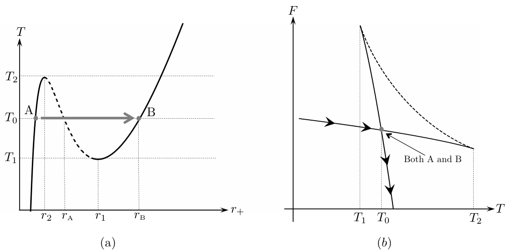
For small temperatures the system has only one value for $r_{+}$. When the temperature is raised to the region $T\in[T_{1},T_{2}]$, the system has three possible values for $r_{+}$. For $T\in[T_{1},T_{0}]$, the smallest value of $r_{+}$ is the one that minimizes the Helmholtz free energy, as it can be seen in Fig.1 (b), and therefore that is the value that the system will choose. When $T=T_{0}$ is reached, the black hole performs a first-order phase transition from point $A$ to point $B$ of Fig.1 (a). This is because at that temperature the two stable branches of the Helmholtz free energy intersect each other, and from that point on, the branch with bigger values of $r_{+}$ minimizes the free energy. The discontinuity in the slope, as one passes from one branch to the other, is precisely the discontinuity in the entropy characterizing a first-order transition.

The idea that the composite of two bosons can become a fermion dates back a long time saha1936origin; Saha:1949np (see also coleman1983magnetic). Basically one notes that the total angular momentum of an electric charge in the presence of a magnetic monopole, even in the non-relativistic limit, must include the contribution from the angular momentum stored in the electromagnetic field. Moreover, because of Dirac’s quantization condition, this effect contributes with half-integer multiples of $\hbar$, so the quantum mechanical system describing the charge/monopole bound state becomes a fermion.

Consider now the ’t Hooft-Polyakov monopole

	$\displaystyle\Phi^{a}$	$\displaystyle=\frac{x^{a}f(vr)}{r^{2}}\,,$		(37)
	$\displaystyle A^{a}_{i}$	$\displaystyle=\frac{\epsilon^{a}_{ij}x^{j}g(vr)}{r^{2}}\,,$
	$\displaystyle A^{a}_{0}$	$\displaystyle=0\,,$

where $f(x)=x\coth(x)-1$, and $g(x)=1-x\,\mathrm{csch}(x)$. Note that this is a four-dimensional example, spatial indices $i,j$ in this case run from $1$ to $3$. The key observation is that this solution does not transform as a vector under spatial rotations nor under global SU(2) transformations, but it does transform correctly under the combination

$$J_{a}=\epsilon_{ai}^{\;\;\;j}\,x^{i}\,p_{j}+t_{a}\,,$$

(38)

where $p_{i}$ is the canonical conjugate to $x^{i}$.

Now consider a non-relativistic spin 0 particle represented by the state $|\psi_{a}\rangle$, where $a$ is an internal isospin index transforming under some irreducible representation of SU(2), interacting with the monopole background (37). Its evolution will be described by a Schrödinger equation $i\partial_{t}|\psi\rangle=H|\psi\rangle$ where $H$ is the Hamiltonian for such particle in the background (37). Since this background transforms as a vector under the $\mathfrak{su(2)}$ generator (38), we get

$$[J_{a},H]=0\,.$$

Thus, we can diagonalize the Hamiltonian using the eigenstates generated by $J^{a}$. Therefore, since the state representing the monopole, say, $|M\rangle$ and the spinless particle $|\psi_{a}\rangle$ are both, independently, multiplets of $SU(2)$, one can think of this scalar-monopole “bound eigenstate”$|M\rangle\otimes|\psi_{a}\rangle$ of $H$ as a state with total angular momentum $J^{a}$ Hasenfratz:1976gr. If the spinless particle $|\psi_{a}\rangle$ is in a half-integer representation of the internal SU(2) group, then the bound state acquires half-integer spin quantum numbers and, by the spin-statistics connection, it effectively becomes a fermion Goldhaber:1976dp. Moreover, Hasenfratz and t’ Hooft Hasenfratz:1976gr also showed that in the classical limit, the angular momentum stored in the Yang-Mills field above is precisely given by the $t_{a}$ contribution in (38).

Consider a complex scalar (multiplet) field $\Phi$ in the black hole (6) and Meron Yang-Mills background (26). Its action reads

$$S_{scalar}=-\frac{1}{2}\int d^{5}x\sqrt{-g}\left[\left(D_{\mu}\Phi\right)^{{\dagger}}D^{\mu}\Phi+m^{2}|\Phi|^{2}\right]\ ,$$

(39)

where $D_{\mu}\equiv\partial_{\mu}+A_{\mu}$, and $\Phi$ is in the fundamental representation of $SU(2)$. Following the logic of Hasenfratz:1976gr, let us now imagine quantizing this scalar field around the classical background of the black hole and Meron field. In other words, defining

	$\displaystyle A_{\mu}$	$\displaystyle=A_{\mu}^{{\rm cl}}+A_{\mu}^{{\rm qu}}\,,$		(40)
	$\displaystyle\Phi$	$\displaystyle=\Phi^{{\rm qu}}\,,$

and by only considering the quantum fluctuations $\Phi^{\rm qu}$ (i.e., neglecting $A_{\mu}^{{\rm qu}}$), one would be quantizing the system in the one-soliton sector of the Hilbert space. That is, our excitations correspond to those of the bound-state formed by the scalar and the Meron background.

In the non-relativistic limit, the interaction of this spinless particle (with internal isospin indices) with such background is described by a Hamiltonian of the form

$$H=-\frac{1}{2m}\gamma^{ij}\left(\nabla_{i}+A_{i}\right)\left(\nabla_{j}+A_{j}\right)\;,\quad i,j=1,2,3,4\,.$$

(41)

where $\gamma^{ij}$ is the inverse of the spatial metric (32), and $A_{i}$ is given by the spatial components of (26). Note that the $A_{i}$’s, and hence $H$, are matrix-valued operators. For simplicity, let us consider the asymptotically flat case $\Lambda=0$. The Hamiltonian has the asymptotic form

$$H_{{\rm asymp}}=-\frac{1}{2m}\partial^{2}_{r}-\frac{1}{2mr^{2}}\,h^{mn}D_{m}D_{n}\,,$$

(42)

where $h^{mn}$ denotes the inverse of the metric on the $S^{3}$ defined in Eq. (25). In order to simplify some calculations, it will prove useful to express the unit three-sphere in terms of cartesian coordinates $X^{M}\,,M=1,2,3,4$ such that $\delta_{MN}X^{M}X^{N}=1$. In these coordinates the metric on $S^{3}$ is $h_{MN}=\delta_{MN}$, and the usual angular momentum operator in four spatial dimensions can be simply expressed as

$$\mathcal{L}_{MN}=-i(x_{M}\partial_{N}-x_{N}\partial_{M})\,.$$

(43)

It is easy to see that this operator does not commute with the Hamiltonian (42). Since partial derivatives transform trivially as vectors under rotations, $r^{2}$ is rotationally invariant, and in this basis $h^{MN}$ is constant (see Appendix C), looking at (42) we see that problem stems from the fact that the gauge connection $A$ does not transform as a vector under rotations generated by (43). Hence, since $\mathcal{L}_{MN}$ is not a conserved quantity, its eigenvalues are not useful to label quantum states. However, the operator

$$\mathcal{J}_{MN}\equiv\mathcal{L}_{MN}+\mathcal{T}_{MN}\,,$$

(44)

does commute with this Hamiltonian provided $\mathcal{T}_{ab}\equiv\epsilon_{\;ab}^{c}t_{c}$ and $\mathcal{T}_{4a}\equiv t_{a}$ (recall that the indices $a,b,c$ run from 1 to 3). Thus, it is $\mathcal{J}_{ij}$ that should be identified with the true angular momentum of the system, and not $\mathcal{L}_{ij}$. This can be seen as follows: expressing the right invariant Maurer-Cartan form (23) in the coordinates $X^{M}$, the Meron field (26) takes the form (see Appendix C)

$$A=A_{M}dX^{M}=A_{a}dX^{a}+A_{4}dX^{4}\,,$$

(45)

where⁴⁴ 4 Even though indices $a,b=1,2,3$ have so far been used as group indices, in (46) they denote spatial indices. This identification between the group manifold and spatial three-sphere is a common ingredient when studying the spin from isospin effect Jackiw:1976xx.

$\displaystyle A_{a}=i\left(X^{4}t_{a}-\epsilon_{\;ab}^{c}X^{b}t_{c}\right)\,,\qquad A_{4}=-iX_{a}t_{a}\,.$

(46)

Using this one obtains

$\displaystyle[\mathcal{J}_{MN},A_{R}]=i\left(\delta_{MR}A_{N}-\delta_{NR}A_{M}\right)\,.$

(47)

Hence, $A_{M}$ rotates as a vector under the action of $\mathcal{J}_{MN}$, and therefore, so does $D_{M}$. Since the asymptotic hamiltonian (42) is quadratic in $D_{M}$, this yields

$$[H_{\rm asymp},\mathcal{J}_{MN}]=0\,,$$

(48)

as promised.

This analysis can be easily generalized to the asymptotically (A)dS case. In fact, in the presence of cosmological constant, the first term in (42) must be replaced by $\frac{3}{\Lambda mr^{2}}\partial^{2}_{r}\,$, which is rotationally invariant as it only depends on $r^{2}$. The second term in (42) remains unmodified and the operators (43) continue to generate the Lorentz subgroup of the full asymptotic symmetry group. As the Meron has support only on $S^{3}$, Eq. (46) also remains unchanged, showing that (48) holds when $\Lambda\neq 0$.

The operator $\mathcal{L}_{MN}$ can be divided into two sets of angular momenta that satisfy the $\mathfrak{su}(2)$ algebra (for details see Appendix B)

$$L^{\pm}_{a}=\epsilon_{a}^{\;bc}\mathcal{L}^{bc}\pm\mathcal{L}_{4a}\,,\quad\left[L^{\pm}_{a},L^{\pm}_{b}\right]=i\epsilon^{c}_{\;ab}L^{\pm}_{c}\,.$$

(49)

In the same way, the total angular momentum $\mathcal{J}_{MN}$ can be divided into two sets of $\mathfrak{su}(2)$ generators, that have the form

$$J^{+}_{a}=L^{+}_{a}+t_{a}\,,\quad J^{-}_{a}=L^{-}_{a}\,.$$

(50)

The form of $J^{+}$ resembles the shift in (38) and produces the spin from isospin effect. Thus, in the same way detailed in subsection 4.1, the bound system of a spinless particle in the background of this meronic black hole can acquire half-integer spin quantum numbers, hence, effectively, becoming a fermion.

It is also instructive to study the Klein-Gordon equation for a scalar field in this background:

$$\left(\square+\nabla_{\mu}A^{\mu}+2A^{\mu}\nabla_{\mu}+A^{\mu}A_{\mu}-m^{2}\right)\Phi=0\,.$$

(51)

After using (6) and (26), Eq. (51) becomes

$$\left[\square-\frac{1}{r^{2}}\left(4\,\vec{t}\cdot\vec{L}^{+}+\vec{t}\cdot\vec{t}\right)-m^{2}\right]\Phi=0\ ,$$

(52)

where $\vec{t}=(t_{1},t_{2},t_{3})$ and $\vec{L}^{+}=(L^{+}_{1},L^{+}_{2},L^{+}_{3})$ is the right angular momentum operator defined in (49) (for details see Appendix A),

	$\displaystyle L_{1}^{+}$	$\displaystyle=i\left(\cos\psi\cot\theta\partial_{\psi}+\sin\psi\partial_{\theta}-\frac{\cos\psi}{\sin\theta}\partial_{\varphi}\right)\,,$
	$\displaystyle L_{2}^{+}$	$\displaystyle=i\left(\sin\psi\cot\theta\partial_{\psi}-\cos\psi\partial_{\theta}-\frac{\sin\psi}{\sin\theta}\partial_{\varphi}\right)\,,$		(53)
	$\displaystyle L_{3}^{+}$	$\displaystyle=-i\partial_{\psi}\,.$

The d’Alembertian on the black hole background (34) has the form

$$\square=-\frac{1}{f^{2}}\partial_{t}^{2}+\frac{1}{r^{3}}\partial_{r}\left(r^{3}f^{2}\partial_{r}\right)-\frac{1}{r^{2}}\mathcal{L}^{2}\,.$$

(54)

Here $\mathcal{L}^{2}$ denotes the square of the four-dimensional angular momentum (43) (see Eq. (89) in Appendix B). Using this and Eq. (50), the equation of motion for the scalar field takes the form

$$\left[-\frac{1}{f^{2}}\partial_{t}^{2}+\frac{1}{r^{3}}\partial_{r}\left(r^{3}f^{2}\partial_{r}\right)-\frac{1}{r^{2}}\left(\mathcal{J}^{2}-\vec{t}\cdot\vec{t}\right)-m^{2}\right]\Phi=0\,,$$

(55)

where $\mathcal{J}^{2}\equiv\frac{1}{2}\mathcal{J}_{MN}\mathcal{J}^{MN}=2\left(J^{+}\right)^{2}+2\left(J^{-}\right)^{2}$ is the square of the total angular momentum (44). Note that the the term $\left(\mathcal{J}^{2}-\vec{t}\cdot\vec{t}\right)$ in Eq. (55) is similar to the one found in Boulware:1976tv, where the scattering of a scalar particle off a magnetic monopole was studied.

Now we can consider modes of the form

$$\Phi_{\ell m_{1}m_{2}}=e^{-i\omega t}D^{\ell}_{m_{1}m_{2}}(\psi,\varphi,\theta)r^{-1}\phi(r)\,,$$

(56)

where $D^{\ell}_{m_{1}m_{2}}(\psi,\varphi,\theta)$ stands for the Wigner D-functions varshalovich1988quantum (see Eq. (81) in Appendix A), which are the higher-dimensional generalization of the standard spherical harmonics meremianin2009hyperspherical. The shift in $L^{+}\rightarrow J^{+}$ produces half-integer shift in the angular momentum eigenvalues of the modes $\Phi_{\ell mn}$ given by (see Eq. (91) in Appendix B),

$$\begin{array}[]{lcl}\mathcal{J}_{34}D^{\ell}_{m_{1}m_{2}}\left(\psi,\theta,\varphi\right)&=&\left(m_{1}-m_{2}+\dfrac{1}{2}\right)D^{\ell}_{m_{1}m_{2}}\left(\psi,\theta,\varphi\right)\,,\\[6.0pt] \mathcal{J}_{12}D^{\ell}_{m_{1}m_{2}}\left(\psi,\theta,\varphi\right)&=&\left(m_{1}+m_{2}+\dfrac{1}{2}\right)D^{\ell}_{m_{1}m_{2}}\left(\psi,\theta,\varphi\right)\,.\end{array}$$

(57)

As the eigenvalues of the total angular momentum $\mathcal{J}_{MN}$ are given by half-integer multiples of $\hbar$, the scalar field $\Phi$ effectively becomes fermionic.

The gauge/gravity duality states that any theory of quantum gravity that asymptotically approaches AdS_d+1 space-time is dual to a flat $d$-dimensional conformal field theory on the boundary of AdS. The AdS/CFT dictionary can be used to relate, in principle, all physical observables of the gravitational theory to those of the CFT.⁵⁵ 5 Although it is not yet clear how the boundary theory precisely reproduces the degrees of freedom of the black hole interior (see Harlow:2018fse for a recent review on the subject), this will not bother us here since we are dealing with fields in the exterior of the black hole only. Because of the strong/weak nature of the correspondence, the description of strongly correlated observables in terms of weakly interacting fields in the gravitational bulk is one of the most useful (and widely studied) aspects of the duality.

In the presence of black holes, the bulk partition function is dual to the thermal partition function of the theory on the boundary, where the Hawking temperature of the black hole corresponds to the temperature of a thermal state in the dual theory. For horizons with spherical topology (such as the one studied here), the dual $\mathcal{N}=4$ super Yang-Mills theory is naturally defined on $S^{d-1}\times\mathbb{R}$ space-time.⁶⁶ 6 However, as noted in Emparan:1999pm, depending on how the radial slices are chosen as one approaches the boundary of (Euclidean) AdS_d+1, one could also have the boundary theory defined on other spacetimes such as $S^{d}$, $\mathbb{R}^{d}$, $\mathbb{H}^{d}$, and $\mathbb{H}^{d-1}\times\mathbb{R}$. Since we now have a new black hole solution at our disposal, a natural question is: what can it do for the dynamics of strongly correlated systems?

In this section we argue that the ‘‘gravitational’’ spin from isospin effect described in the previous section has the interesting property of describing fermionic observables in the boundary of the spacetime⁷⁷ 7 We note that this boundary effect is not restricted to the asymptotically AdS case only, but also for asymptotically dS and Minskowski. This could have interesting applications in cosmology (dS) and also in the recent developments of amplitudes on the celestial sphere., even though the bulk theory is purely bosonic.⁸⁸ 8 The converse case, i.e., finding the gravitational dual of the usual flat space spin from isospin effect, is also an interesting question which we leave for future work. We will provide supporting evidence that the composite system of a scalar field and the Meron black hole is dual to a fermionic operator in the boundary CFT. Moreover, we also conjecture that this corresponds to a double trace CFT operator.

The first argument is that scalar excitations, in the presence of the Meron black hole, manifest themselves as fermionic degrees of freedom at the AdS boundary. This stems from the fact that the total angular momentum (44) has half-integer quantum numbers. However, there is a more direct way to see this. For our black hole solution (29) with $\Lambda\equiv-6/L^{2}<0$, the metric is asymptotically $AdS_{5}$ and, as $r\to\infty$, we get

$$ds^{2}\sim\frac{r^{2}}{L^{2}}\left(-dt^{2}+L^{2}h_{mn}dx^{m}dx^{n}\right)\,,$$

(58)

which defines the metric of the conformal boundary, with topology $\mathbb{R}\times S^{3}$. Consider now the expansion of the scalar field $\Phi$ near the spatial boundary ($r\to\infty$). We look for an Ansatz of the form (see, e.g., deHaro:2000vlm; Skenderis:2002wp)

$\displaystyle\Phi(r,x)=r^{-\Delta}\left(\varphi^{(0)}(x)+\frac{1}{r^{2}}\varphi^{(2)}(x)+\cdots\right)$

(59)

where $x$ are the coordinates of the fields that “live” on the boundary of $AdS_{5}$. Since this boundary has the topology $\mathbb{R}\times S^{3}$, we use $x=(t,\Omega)$ where $\Omega$ collectively refers to the three angular coordinates on the 3-sphere (see equations (24) and (25)). Inserting the asymptotic expansion (59) into the scalar wave equation (55) one obtains (at leading order in the large $r$ expansion)

$$\Delta(\Delta-4)-m^{2}L^{2}=0\,.$$

(60)

This is the standard relation between the mass of the scalar field in five dimensions and $\Delta$, which is interpreted as the conformal dimension of the scalar CFT operator dual to $\Phi$. The subleading term yields

$$\left[-\partial_{t}^{2}-\frac{1}{L^{2}}(\mathcal{J}^{2}-\vec{t}\cdot\vec{t})\right]\varphi^{(0)}(t,\Omega)=\frac{4(1-\Delta)}{L^{4}}\varphi^{(2)}(t,\Omega)\,.$$

(61)

In the absence of the Meron, $\mathcal{J}^{2}=\mathcal{L}^{2}=-\nabla^{2}_{S^{3}}$ and $\vec{t}=0$, thus $\varphi^{(0)}$ would represent a massless scalar field in four spacetime dimensions moving on a 3-sphere coupled to the source $\varphi^{(2)}(t,\Omega)$. Turning on the Meron gauge field in the bulk, however, yields equation (61) with the total angular momentum $\mathcal{J}$ acquiring an extra term (see (44)) due to the coupling between the isospin indices of $\Phi$ and the Meron. We can re-write the equation above as

$$\left[-\partial_{t}^{2}+\frac{1}{L^{2}}h^{mn}\left(\nabla_{m}+A_{m}\right)\left(\partial_{n}+A_{n}\right)\right]\varphi^{(0)}=\frac{4(1-\Delta)}{L^{4}}\varphi^{(2)}\,,$$

(62)

where $\nabla_{m}$ is the covariant derivative with respect to the affine connection on $S^{3}$, and $A_{m}$ denotes the angular components of the Meron gauge field (26)⁹⁹ 9 Equation (62) also appears in the description of scalar fields with generalized Wentzell boundary conditions Zahn:2015due; Dappiaggi:2018pju.. Due to the topological nature of our Meron $A_{\mu}$ (which extends all the way to infinity), and because we are studying the scalar field in the probe limit, one can consider the Meron as an external field which couples to the boundary degrees of freedom of the scalar (isospin doublet) $\Phi$.

Now we will see that equation (62) can actually be reinterpreted as describing fermionic degrees of freedom. In order to do this, let us consider a Majorana fermion in the chiral representation,

$$\Psi=\left(\begin{array}[]{c}\psi\\ -i\sigma_{2}\psi^{*}\end{array}\right)\,,$$

(63)

defined on $\mathbb{R}\times S^{3}$ (see for instance, Pal:2010ih; Dvornikov:2011bu; henn2014scattering). This, in turn, can be described in terms of the two-spinor $\psi$ satisfying a massive Weyl equation (see Appendix D). Adding a source term $\rho_{\psi}$ for $\psi$, the equation becomes

$$\partial_{t}\psi-e^{m}_{a}\sigma^{a}\left(\partial_{m}+\Gamma_{m}\right)\psi+\mu\,\sigma_{2}\psi^{*}=-\rho_{\psi}\,,$$

(64)

where $\sigma^{a}$ are the Pauli matrices, $e_{a}^{m}$ denote the inverse dreibein associated to the metric (25), and $\Gamma_{m}$ is the spin connection on $S^{3}$. If we consider the corresponding Klein-Gordon equation for the two-spinor $\psi$ (see Eq. (107)), one obtains

$$\left[-\partial_{t}^{2}+\frac{1}{L^{2}}h^{mn}\left(\nabla_{m}+\Gamma_{m}\right)\left(\partial_{n}+\Gamma_{n}\right)+\frac{3}{2L^{2}}-\mu^{2}\right]\psi=-\rho\,.$$

(65)

where the right hand side of Eq. (65) can be written in terms of $\rho_{\psi}$ and its derivatives, but the explicit form is not important here. Notice that equation (65) does not make any reference to a gauge field coupling. Nevertheless, using Eqs. (103) and (104), it is straightforward to see that, on $S^{3}$, the components of the spin connection $\Gamma_{m}$ match the angular components of the Meron gauge field (10) (for $\lambda=1/2$)

$$\Gamma_{m}\,dx^{m}=\frac{i}{4}\omega_{R}^{a}\sigma_{a}=A_{m}dx^{m}\,.$$

(66)

Thus, (65) is on-shell equivalent to (62) when $\psi$ is identified with $\varphi^{(0)}$, the source term $\rho$ is identified with $\frac{4(1-\Delta)}{L^{4}}\varphi^{(2)}$, and the mass of the Majorana fermion is fixed to $\mu^{2}=3/2L^{2}$. This means that the original scalar excitations of an isospin doublet $\Phi$, coupled to the Meron gauge field through its isospin indices, can be reinterpreted as a two-spinor $\psi$ with fixed mass, coupled to the geometry of the $AdS_{5}$ conformal boundary and satisfying (65). Hence, knowing a solution of (62), allows us to construct a Majorana spinor at the boundary by means of (63) by reinterpreting isospin indices of $\Phi$ as spin indices. This argument is another way to justify why the Wigner D-functions in the modes (56) must be chosen as fermionic, pretty much in the same way as it happens when describing fermions in terms of the Skyme model Adkins:1983ya (see also Rho:1994ni). All this put together signals that there must be a way to construct a holographic dictionary between a purely bosonic theory in the bulk and a fermionc theory at the boundary using the spin from isospin effect. It is important to note that, even though we expect the Meron-scalar bound state to be a fermion, the fact that the probe scalar field has no back reaction means we are considering its mass to be very small compared to the mass of the Meron black hole. Thus, in this limit, the properties of the fermionic bound state can be approximated by the dynamics of the scalar field only, which is tantamount to studying the properties of the hydrogen atom in the limit when the proton is fixed at the origin because it is much heavier than the electron.

A stronger argument in support of this idea is the following. The GKPW dictionary Gubser:1998bc; Witten:1998qj states that the asymptotic value of $\Phi(x,r)$ at the AdS boundary ($r\to\infty$) acts as the source for a scalar operator in the CFT. Since $\Phi$ is a bulk scalar, its asymptotic value is dual to a scalar operator $\mathcal{O}^{a}$ in the 4-dimensional CFT Gubser:1998bc; Witten:1998qj. Near the boundary ($r\to\infty$) the scalar field behaves as given in (59). It is standard to regard $\varphi^{(0)}$ as the source for the operators $\mathcal{O}^{a}$ of the CFT, which in turn yields $\varphi^{(2)}$ to be directly proportional to their vacuum expectation value $\langle\mathcal{O}^{a}\rangle$. From (55) it is easy to see that, at leading order, the asymptotic behavior of the scalar field near the boundary is insensitive to the presence of the gauge field $A_{\mu}$. This is simply because the term that accompanies $\mathcal{L}^{2}$ in the Klein-Gordon equation, which gets modified as

$$\mathcal{L}^{2}\to\mathcal{J}^{2}-\vec{t}\cdot\vec{t}\,,$$

is subleading in the large $r$ expansion. Thus, one may wonder in what sense the “spin from isospin” effect modifies the CFT observables. It has, however, an immediate effect. In order to see this, it is useful to use the identification between two Fock spaces: the space of (spinless) free particle states in AdS and the space of states in the CFT Witten:1998qj; Balasubramanian:1998de; Balasubramanian:1998sn; Balasubramanian:1999ri (see also Fitzpatrick:2010zm; Fitzpatrick:2011jn).¹⁰¹⁰ 10 At leading order in the $1/N$ expansion in the CFT, this identification is exact. This is indeed all we need since subleading corrections in $1/N$ correspond to stringy corrections to the effective gravitational theory which we are not considering here. In the $AdS_{5}$ description, a free scalar field $\Phi$ can be written as

$\displaystyle\Phi=\sum_{n,\ell,m_{1},m_{2}}\Phi^{n}_{\ell m_{1}m_{2}}\,a^{n}_{\ell m_{1}m_{2}}+\Phi^{n\,*}_{\ell m_{1}m_{2}}\,a^{n\,\dagger}_{\ell m_{1}m_{2}}\,,$

(67)

where the modes $\Phi^{n}_{\ell m_{1}m_{2}}$ satisfy the wave equation (55), $n$ is their energy eigenvalue, $\ell$ is the total angular momentum quantum number, while $m_{1},m_{2}$ are the “magnetic” angular momentum quantum numbers that arise from the $S^{3}$ of $AdS_{5}$ (e.g., in $AdS_{4}$, they would simply be the usual “$m$” eigenvalue of $L_{z}$ of three spatial dimensions). Because of our hedgehog-type solution for the gauge field (26), the CFT at the boundary of $AdS_{5}$ is naturally defined on $S^{3}$. Now, the boundary operator $\mathcal{O}$, dual to $\Phi$, inherits a similar decomposition which, in Lorentzian radial quantization, has the form

$\displaystyle\mathcal{O}(t,\Omega)=\sum_{n,\ell,m_{1},m_{2}}\frac{1}{N_{n\ell m_{1}m_{2}}^{\mathcal{O}}}\left[e^{i(2\Delta+2n+\ell)t}Y^{\ell}_{m_{1}m_{2}}(\Omega)a^{n}_{\ell m_{1}m_{2}}+e^{-i(2n+\ell)t}Y^{\ell\,*}_{m_{1}m_{2}}(\Omega)a^{n\,\dagger}_{\ell m_{1}m_{2}}\right]\,,$

(68)

where $(t,\Omega)$ are the spacetime coordinates of the 4-dimensional CFT, $\Delta$ is the conformal dimension of the operator $\mathcal{O}$, $N_{n\ell m_{1}m_{2}}^{\mathcal{O}}$ is a normalization factor, and $Y^{\ell}_{m_{1}m_{2}}(\Omega)$ are the spherical harmonics on $S^{3}$. The crucial point is the following: as discussed in Section 4.2, turning on the Meron field in the bulk shifts the eigenvalues of the total angular momentum $\mathcal{J}$ by half-integer numbers as in (57) (provided the scalar field is in one of the half-integer representations of SU(2) of isospin). Therefore, the spherical harmonics $Y^{\ell}_{m_{1}m_{2}}$ in (68), which (for $AdS_{5}$) are just the Wigner D-functions (56), will also see its angular momentum quantum numbers ($m_{1},m_{2}$) shifted by $\pm 1/2$ (see Eq. (57)), making the putative scalar $\mathcal{O}$ in (68) now a fermionic operator! ¹¹¹¹ 11 As a consequence, there will be no “s-wave” since the eigenvalues of $\mathcal{J}$ would never vanish.

References

- (1) N. Manton and P. Sutcliffe, Topological solitons. Cambridge University Press, 2004.
- (2) J. Greensite, An Introduction to the Confinement Problem. Springer, 2010.
- (3) R. Jackiw and C. Rebbi, Spin from Isospin in a Gauge Theory, Phys. Rev. Lett. 36 (1976) 1116.
- (4) P. Hasenfratz and G. ’t Hooft, A Fermion-Boson Puzzle in a Gauge Theory, Phys. Rev. Lett. 36 (1976) 1119.
- (5) A. S. Goldhaber, Spin and Statistics Connection for Charge-Monopole Composites, Phys. Rev. Lett. 36 (1976) 1122.
- (6) F. Canfora, F. Correa, A. Giacomini and J. Oliva, Exact meron Black Holes in four dimensional SU(2) Einstein-Yang-Mills theory, Phys. Lett. B722 (2013) 364 [1208.6042].
- (7) P. Cordero and C. Teitelboim, Hamiltonian Treatment of the Spherically Symmetric Einstein Yang-Mills System, Annals Phys. 100 (1976) 607.
- (8) P. Bizon, Colored black holes, Phys. Rev. Lett. 64 (1990) 2844.
- (9) H. Künzle and A. Masood-ul Alam, Spherically symmetric static su (2) einstein–yang–mills fields, Journal of Mathematical Physics 31 (1990) 928.
- (10) M. S. Volkov and D. V. Gal’tsov, Gravitating nonAbelian solitons and black holes with Yang-Mills fields, Phys. Rept. 319 (1999) 1 [hep-th/9810070].
- (11) Y. Brihaye, A. Chakrabarti, B. Hartmann and D. H. Tchrakian, Higher order curvature generalizations of Bartnick-McKinnon and colored black hole solutions in D = 5, Phys. Lett. B561 (2003) 161 [hep-th/0212288].
- (12) N. Okuyama and K.-i. Maeda, Five-dimensional black hole and particle solution with nonAbelian gauge field, Phys. Rev. D67 (2003) 104012 [gr-qc/0212022].
- (13) G. W. Gibbons and P. K. Townsend, Self-gravitating Yang Monopoles in all Dimensions, Class. Quant. Grav. 23 (2006) 4873 [hep-th/0604024].
- (14) Y. Brihaye and E. Radu, Magnetic solutions in AdS(5) and trace anomalies, Phys. Lett. B658 (2008) 164 [0706.4378].
- (15) E. Winstanley, Classical Yang-Mills black hole hair in anti-de Sitter space, Lect. Notes Phys. 769 (2009) 49 [0801.0527].
- (16) S. H. Mazharimousavi and M. Halilsoy, Einstein-Yang-Mills black hole solution in higher dimensions by the Wu-Yang Ansatz, Phys. Lett. B659 (2008) 471 [0801.1554].
- (17) N. Bostani and M. H. Dehghani, Topological Black Holes of (n+1)-dimensional Einstein-Yang-Mills Gravity, Mod. Phys. Lett. A25 (2010) 1507 [0908.0661].
- (18) M. Agop and E. Radu, Ricci flat black holes in higher dimensional SU(2) Einstein-Yang-Mills theory with negative cosmological constant, Phys. Lett. B688 (2010) 88.
- (19) E. Winstanley, A menagerie of hairy black holes, Springer Proc. Phys. 208 (2018) 39 [1510.01669].
- (20) M. S. Volkov, Hairy black holes in the XX-th and XXI-st centuries, in Proceedings, 14th Marcel Grossmann Meeting on Recent Developments in Theoretical and Experimental General Relativity, Astrophysics, and Relativistic Field Theories (MG14) (In 4 Volumes): Rome, Italy, July 12-18, 2015, vol. 2, pp. 1779–1798, 2017, 1601.08230, DOI.
- (21) B. L. Shepherd and E. Winstanley, Black holes with gauge field hair and superconducting horizons, JHEP 01 (2017) 065 [1611.04162].
- (22) M. Sadeghi, Einstein-Yang-Mills AdS black brane solution in massive gravity and viscosity bound, Eur. Phys. J. C78 (2018) 875 [1810.09242].
- (23) V. de Alfaro, S. Fubini and G. Furlan, A New Classical Solution of the Yang-Mills Field Equations, Phys. Lett. B65 (1976) 163.
- (24) C. G. Callan, Jr., R. F. Dashen and D. J. Gross, Toward a Theory of the Strong Interactions, Phys. Rev. D17 (1978) 2717.
- (25) C. G. Callan, Jr., R. F. Dashen and D. J. Gross, A Mechanism for Quark Confinement, Phys. Lett. B66 (1977) 375.
- (26) J. Glimm and A. M. Jaffe, Meron Pairs and Quark Confinement, Phys. Rev. Lett. 40 (1978) 277.
- (27) C. G. Callan, Jr., R. F. Dashen and D. J. Gross, A Theory of Hadronic Structure, Phys. Rev. D19 (1979) 1826.
- (28) A. Actor, Classical Solutions of SU(2) Yang-Mills Theories, Rev. Mod. Phys. 51 (1979) 461.
- (29) F. Lenz, J. W. Negele and M. Thies, Confinement from merons, Phys. Rev. D69 (2004) 074009 [hep-th/0306105].
- (30) F. Canfora and P. Salgado-Rebolledo, Generalized hedgehog ansatz and Gribov copies in regions with nontrivial topologies, Phys. Rev. D87 (2013) 045023 [1302.1264].
- (31) F. Canfora and H. Maeda, Hedgehog ansatz and its generalization for self-gravitating Skyrmions, Phys. Rev. D87 (2013) 084049 [1302.3232].
- (32) F. Canfora, Nonlinear superposition law and Skyrme crystals, Phys. Rev. D88 (2013) 065028 [1307.0211].
- (33) S. Chen, Y. Li and Y. Yang, Exact Kink Solitons in Skyrme Crystals, Phys. Rev. D89 (2014) 025007 [1312.2479].
- (34) F. Canfora, F. Correa and J. Zanelli, Exact multisoliton solutions in the four-dimensional Skyrme model, Phys. Rev. D90 (2014) 085002 [1406.4136].
- (35) F. Canfora, A. Giacomini and S. A. Pavluchenko, Cosmological dynamics of gravitating hadron matter, Phys. Rev. D90 (2014) 043516 [1406.1541].
- (36) F. Canfora and G. Tallarita, Constraining Monopoles by Topology: an Autonomous System, JHEP 09 (2014) 136 [1407.0609].
- (37) F. Canfora, M. Di Mauro, M. A. Kurkov and A. Naddeo, SU(N) multi-Skyrmions at Finite Volume, Eur. Phys. J. C75 (2015) 443 [1508.07055].
- (38) S. Chen and Y. Yang, Domain Wall Equations, Hessian of Superpotential, and Bogomol’nyi Bounds, Nucl. Phys. B904 (2016) 470 [1512.04080].
- (39) E. Ayon-Beato, F. Canfora and J. Zanelli, Analytic self-gravitating Skyrmions, cosmological bounces and AdS wormholes, Phys. Lett. B752 (2016) 201 [1509.02659].
- (40) F. Canfora and G. Tallarita, BPS Monopoles in , Phys. Rev. D91 (2015) 085033 [1502.02957].
- (41) F. Canfora and G. Tallarita, Multi-Skyrmions with orientational moduli, Phys. Rev. D94 (2016) 025037 [1607.04140].
- (42) G. Tallarita and F. Canfora, Multi-Skyrmions on , Rational maps and Popcorn Transitions, Nucl. Phys. B921 (2017) 394 [1706.01397].
- (43) F. Canfora, A. Paliathanasis, T. Taves and J. Zanelli, Cosmological Einstein-Skyrme solutions with nonvanishing topological charge, Phys. Rev. D95 (2017) 065032 [1703.04860].
- (44) F. Canfora, N. Dimakis and A. Paliathanasis, Topologically nontrivial configurations in the 4d Einstein-nonlinear -model system, Phys. Rev. D96 (2017) 025021 [1707.02270].
- (45) F. Canfora, S. H. Oh and P. Salgado-Rebolledo, Gravitational catalysis of merons in Einstein-Yang-Mills theory, Phys. Rev. D96 (2017) 084038 [1710.00133].
- (46) E. Witten, Anti-de Sitter space and holography, Adv. Theor. Math. Phys. 2 (1998) 253 [hep-th/9802150].
- (47) V. Balasubramanian, P. Kraus, A. E. Lawrence and S. P. Trivedi, Holographic probes of anti-de Sitter space-times, Phys. Rev. D59 (1999) 104021 [hep-th/9808017].
- (48) V. Balasubramanian, P. Kraus and A. E. Lawrence, Bulk versus boundary dynamics in anti-de Sitter space-time, Phys. Rev. D59 (1999) 046003 [hep-th/9805171].
- (49) V. Balasubramanian, S. B. Giddings and A. E. Lawrence, What do CFTs tell us about Anti-de Sitter space-times?, JHEP 03 (1999) 001 [hep-th/9902052].
- (50) S. A. Hartnoll, A. Lucas and S. Sachdev, Holographic quantum matter, 1612.07324.
- (51) S. S. Gubser, Breaking an Abelian gauge symmetry near a black hole horizon, Phys. Rev. D78 (2008) 065034 [0801.2977].
- (52) I. R. Klebanov and M. J. Strassler, Supergravity and a confining gauge theory: Duality cascades and chi SB resolution of naked singularities, JHEP 08 (2000) 052 [hep-th/0007191].
- (53) I. R. Klebanov and N. A. Nekrasov, Gravity duals of fractional branes and logarithmic RG flow, Nucl. Phys. B574 (2000) 263 [hep-th/9911096].
- (54) R. L. Arnowitt, S. Deser and C. W. Misner, The Dynamics of general relativity, Gen. Rel. Grav. 40 (2008) 1997 [gr-qc/0405109].
- (55) A. J. Hanson, T. Regge and C. Teitelboim, Constrained Hamiltonian Systems. Accademia Nazionale dei Lincei, 1976.
- (56) M. Henneaux and C. Teitelboim, Hamiltonian treatment of asymptotically anti-de Sitter spaces, Phys. Lett. B142 (1984) 355.
- (57) A. Gomberoff and C. Teitelboim, de Sitter black holes with either of the two horizons as a boundary, Phys. Rev. D67 (2003) 104024 [hep-th/0302204].
- (58) M. Banados, C. Teitelboim and J. Zanelli, The Black hole in three-dimensional space-time, Phys. Rev. Lett. 69 (1992) 1849 [hep-th/9204099].
- (59) M. Banados, M. Henneaux, C. Teitelboim and J. Zanelli, Geometry of the (2+1) black hole, Phys. Rev. D48 (1993) 1506 [gr-qc/9302012].
- (60) S. R. Coleman and F. De Luccia, Gravitational Effects on and of Vacuum Decay, Phys.Rev. D21 (1980) 3305.
- (61) J. Louko and S. N. Winters-Hilt, Hamiltonian thermodynamics of the Reissner-Nordstrom anti-de Sitter black hole, Phys. Rev. D54 (1996) 2647 [gr-qc/9602003].
- (62) A. Chamblin, R. Emparan, C. V. Johnson and R. C. Myers, Charged AdS black holes and catastrophic holography, Phys. Rev. D60 (1999) 064018 [hep-th/9902170].
- (63) M. N. Saha, The origin of mass in neutrons and protons, Indian J. Phys. 10 (1936) 141.
- (64) M. N. Saha, Note on Dirac’s theory of magnetic poles, Phys. Rev. 75 (1949) 1968.
- (65) S. Coleman, The magnetic monopole fifty years later, in The unity of the fundamental interactions, pp. 21–117, Springer, (1983).
- (66) D. G. Boulware, L. S. Brown, R. N. Cahn, S. D. Ellis and C.-k. Lee, Scattering on Magnetic Charge, Phys. Rev. D14 (1976) 2708.
- (67) D. A. Varshalovich, A. N. Moskalev and V. K. Khersonskii, Quantum theory of angular momentum. World Scientific, 1988.
- (68) A. Meremianin, Hyperspherical harmonics with arbitrary arguments, Journal of Mathematical Physics 50 (2009) 013526.
- (69) D. Harlow, TASI Lectures on the Emergence of Bulk Physics in AdS/CFT, PoS TASI2017 (2018) 002 [1802.01040].
- (70) R. Emparan, C. V. Johnson and R. C. Myers, Surface terms as counterterms in the AdS / CFT correspondence, Phys. Rev. D60 (1999) 104001 [hep-th/9903238].
- (71) S. de Haro, S. N. Solodukhin and K. Skenderis, Holographic reconstruction of space-time and renormalization in the AdS / CFT correspondence, Commun. Math. Phys. 217 (2001) 595 [hep-th/0002230].
- (72) K. Skenderis, Lecture notes on holographic renormalization, Class. Quant. Grav. 19 (2002) 5849 [hep-th/0209067].
- (73) J. Zahn, Generalized Wentzell boundary conditions and quantum field theory, Annales Henri Poincare 19 (2018) 163 [1512.05512].
- (74) C. Dappiaggi, H. R. C. Ferreira and B. A. Juárez-Aubry, Mode solutions for a Klein-Gordon field in anti–de Sitter spacetime with dynamical boundary conditions of Wentzell type, Phys. Rev. D97 (2018) 085022 [1802.00283].
- (75) P. B. Pal, Dirac, Majorana and Weyl fermions, Am. J. Phys. 79 (2011) 485 [1006.1718].
- (76) M. Dvornikov, Canonical quantization of a massive Weyl field, Found. Phys. 42 (2012) 1469 [1106.3303].
- (77) J. M. Henn and J. C. Plefka, Scattering amplitudes in gauge theories, vol. 883. Springer, 2014.
- (78) G. S. Adkins, C. R. Nappi and E. Witten, Static Properties of Nucleons in the Skyrme Model, Nucl. Phys. B228 (1983) 552.
- (79) M. Rho, The Cheshire Cat Hadrons Revisited, hep-ph/0206003.
- (80) S. S. Gubser, I. R. Klebanov and A. M. Polyakov, Gauge theory correlators from noncritical string theory, Phys. Lett. B428 (1998) 105 [hep-th/9802109].
- (81) A. L. Fitzpatrick, E. Katz, D. Poland and D. Simmons-Duffin, Effective Conformal Theory and the Flat-Space Limit of AdS, JHEP 07 (2011) 023 [1007.2412].
- (82) A. L. Fitzpatrick and J. Kaplan, Scattering States in AdS/CFT, 1104.2597.
- (83) E. Witten, Multitrace operators, boundary conditions, and AdS / CFT correspondence, hep-th/0112258.
- (84) D. T. Son and A. O. Starinets, Minkowski space correlators in AdS / CFT correspondence: Recipe and applications, JHEP 09 (2002) 042 [hep-th/0205051].
- (85) C. P. Herzog and D. T. Son, Schwinger-Keldysh propagators from AdS/CFT correspondence, JHEP 03 (2003) 046 [hep-th/0212072].
- (86) D. Marolf, States and boundary terms: Subtleties of Lorentzian AdS / CFT, JHEP 05 (2005) 042 [hep-th/0412032].
- (87) S. S. Gubser, S. S. Pufu and F. D. Rocha, Bulk viscosity of strongly coupled plasmas with holographic duals, JHEP 08 (2008) 085 [0806.0407].
- (88) K. Skenderis and B. C. van Rees, Real-time gauge/gravity duality: Prescription, Renormalization and Examples, JHEP 05 (2009) 085 [0812.2909].
- (89) N. Iqbal and H. Liu, Universality of the hydrodynamic limit in AdS/CFT and the membrane paradigm, Phys. Rev. D79 (2009) 025023 [0809.3808].
- (90) M. Henneaux, Boundary terms in the AdS / CFT correspondence for spinor fields, in Mathematical methods in modern theoretical physics. Proceedings, International Meeting, School and Workshop, ISPM’98, Tbilisi, Georgia, September 5-18, 1998, pp. 161–170, 1998, hep-th/9902137.
- (91) N. Iqbal and H. Liu, Real-time response in AdS/CFT with application to spinors, Fortsch. Phys. 57 (2009) 367 [0903.2596].
- (92) M. Henningson and K. Sfetsos, Spinors and the AdS / CFT correspondence, Phys. Lett. B431 (1998) 63 [hep-th/9803251].
- (93) W. Mueck and K. S. Viswanathan, Conformal field theory correlators from classical field theory on anti-de Sitter space. 2. Vector and spinor fields, Phys. Rev. D58 (1998) 106006 [hep-th/9805145].
- (94) J. Milnor, On fundamental groups of complete affinely flat manifolds, Advances in Mathematics 25 (1977) 178.
- (95) C. R. Frye and C. J. Efthimiou, Spherical Harmonics in p Dimensions, 1205.3548.